GSJ: Volume 7, Issue 1,
January
2019, Online: ISSN
2320
-9186
www.globalscientificjournal.com
L
INDLEY
S
TRETCHED
E
XPONENTIAL
D
ISTRIBUTION WITH
A
PPLICATIONS
Gulshan Ara Majid
Department of Statistics, Lahore Garrison University, DHA, Lahore, Pakistan.
Ahmad Saeed Akhter
College of Statistical and Actuarial Sciences, University of the Punjab, Lahore, Pakistan.
Abstract
In this paper, we have introduced an innovative generalization of the Stretched Exponential distribution termed as the Lindley Generalized Stretched Exponential distribution. This proposed distribution can model data in form of decreasing and increasing hazard rates. Besides, we have derived some mathematical properties of the distribution covering probability density function, distribution function, survival, failure rate and reversed hazard functions, moments, moment generating function, cumulant generating function, Renyi entropy of introduced distribution. The Maximum Likelihood method has been used for estimation of parameters. We have used real life data sets to demonstrate the worth and significance of introduced distribution. It has been observed that the introduced distribution of three parameters fits better than its specific cases as well as competitive distributions for all data sets.
Keywords.
Lindley distribution, Stretched Exponential distribution, Generalized,1.
Introduction
The Lindley distribution was firstly proposed by Lindley (1958) in the contextual of Bayesian statistics i.e. counter example of Fudicial Statistics that was mixture of Exponential and Gamma distributions. The Lindley distribution is used to explain the lifetime of a device or process. It can be used in extensive areas, including Engineering, Biology, Medicine, Ecology and Finance. Ghitany et. al (2011) stated that it’s mainly useful for modelling in mortality studies.
The generalized form of a distribution can be introduced and offered more flexible distribution for modelling real life data. Technique of transformation can be adopted to create Lindley Stretched Exponential distribution for desired purpose. That is Stretched Exponential distribution is transformed into Lindley distribution.
The statistical literature’s point of view, the Lindley distribution has generated little attention in excess of the eminent Exponential distribution because these have closed form as well as approach of comparison. In this connection, one improvement of the Lindely distribution is to make a comparison to the exponential distribution. That’s why; the Exponential distribution has constant mean residual life function and hazard rate however the Lindley distribution has decreasing mean residual life function and increasing hazard rate.
Some researchers have presented new classes of distributions on basis of modifications of the Lindley distribution along with their properties. The chief awareness is constantly focussed by inserting former and existing distributions to create innovative flexible structures. Many forms of Lindley distribution were described in “A two-parameter form” (Shanker et al
2013), A two-parameter weighted form (Ghitany et al 2011), An extended (EL) distribution (Bakouch et al 2012), An Exponential Geometric distribution (Adamidis and Loukas 1998). The transmuted Lindley-Geometric Distribution (Merovci, and Elbatal). Sankaran (1970) presented the discrete Poisson–Lindley distribution by joining the Poisson and Lindley distributions. Mahmoudi and Zakerzadeh (2010) introduced an extended version of the compound Poisson distribution by combining the Poisson distribution with the generalized Lindley distribution. Louzada, Roman, and Cancho (2011) suggested the complementary exponential geometric distribution by compounding the geometric and the exponential distributions.
The purpose of this paper is to present an extension of the Lindley distribution which offers a more flexible distribution for modelling any real life data. The innovative distribution can assist decreasing and increasing failure rates as well as unimodal. We present the Lindley Generalized Stretched Exponential distribution (LGSED) by transformation.
generating function and renyi’ entropy. Section 5 deals with the maximum likelihood estimates for the parameters of the distribution. To conclude the distribution, the real life data applications of the newly developed distribution have provided in section 6.
2.
Density, Distribution Functions
A random variable X is said to have Lindley distribution (θ), if its probability density function (pdf) and distribution function (cdf) are defined respectively as:
( ) ( )
(1)
( ) ( )
(2)
By using transformation, {( ) } , the above pdf and cdf of Lindley distribution are transformed into Lindley Generalized Stretched Exponential (LGSE) distribution, then its probability density function and cumulative distribution function will be obtained by.
( )
( ) {( ) }
( ) [ {( ) } ] {( ) }
. (3)
also,
( )
{( ) }
[ {( ) } ]
(4)
Figure 1: Plots of LGSE density function and distribution function for fixed values of (a, b, c) = 1 with different values of
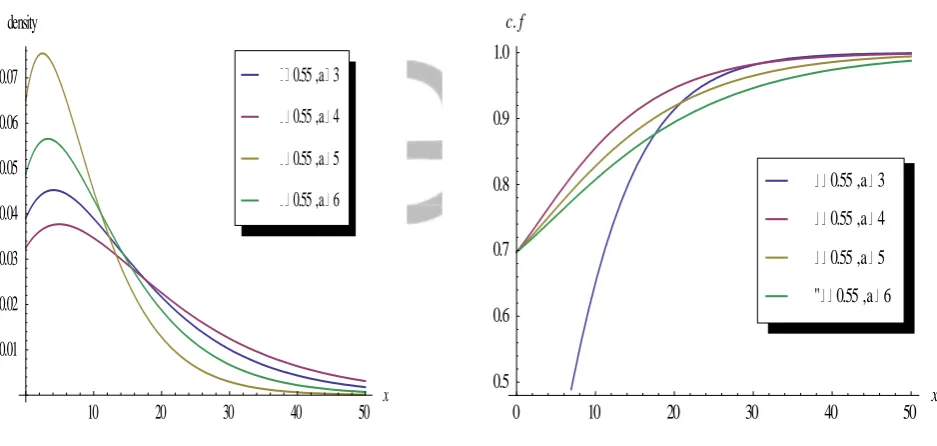
Figure 2: Plots of LGSE density function and distribution function for fixed values of θ = 0.55 (b, c) = 1 with different values of
2 4 6 8 10 12 x
0.1 0.2 0.3 0.4 0.5
density
0.55 0.75 0.9 1
2 4 6 8 10 12 x
0.6 0.7 0.8 0.9 1.0
c.f
0.55 0.75 0.9 1
10 20 30 40 50 x 0.01
0.02 0.03 0.04 0.05 0.06 0.07
density
0.55 ,a 6 0.55 ,a 5 0.55 ,a 4 0.55 ,a 3
0 10 20 30 40 50 x
0.5 0.6 0.7 0.8 0.9 1.0
c.f
Figure 3: Plots of LGSE density function and distribution function for fixed values of b = 2, c = 1 with different values of and θ.
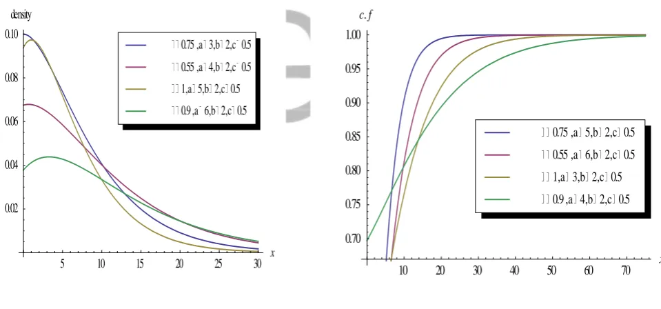
Figure 4: Plots of LGSE density function and distribution function for fixed values of b = 2, c = 0.5 with different values of and .
From all above Figures, it is observed that distribution shows Lindley exponential behaviour and unimodal.
5 10 15 20 x
0.05 0.10 0.15 0.20
density
1,a 5,b 2,c 1 0.9 ,a 6,b 2,c 1 0.75 ,a 3,b 2,c 1 0.55 ,a 4,b 2,c 1
0 5 10 15 20 25 30 35 x
0.5 0.6 0.7 0.8 0.9 1.0
c.f
1,a 5,b 2,c 1 0.9 ,a 6,b 2,c 1 0.75 ,a 3,b 2,c 1 0.55 ,a 4,b 2,c 1
5 10 15 20 25 30 x
0.02 0.04 0.06 0.08 0.10
density
0.9 ,a 6,b 2,c 0.5 1,a 5,b 2,c 0.5 0.55 ,a 4,b 2,c 0.5 0.75 ,a 3,b 2,c 0.5
10 20 30 40 50 60 70 x
0.70 0.75 0.80 0.85 0.90 0.95 1.00
c.f
2.1.
Special Cases
We can find some existing models through appropriate range of parameters. This particular choice of parameters can fit the observed data too. Consequently, certain Specific cases of
LGSEdistributionare discussed below by replacing different values of and
2.1.1. By replacing in Equation (3), we get three parameter Lindley Stretched Exponential distribution (LSED).
( )
( )( )
{ ( ) } ( )
( ) . (5)
2.1.2. By replacing in Equation (3), we get two parameter Lindley Exponential distribution (LED).
( ) ( )( ) ( )
. (6)
2.1.3. By replacing in Equation (3), we get two parameter Lindley Negative Exponential distribution (LNED).
( )
( )( ) .
(7) 2.1.4. By replacing in Equation (3), we get one
parameter Lindley distribution (LD). ( )
( )( )
. (8)
3.
Survival, Hazard and Reverse Hazard Functions
A random variable X is said to have Lindley Stretched Exponential distribution with probability density function (pdf), ( ), i.e. (3) and distribution function (cdf), ( ), i.e. (4), then the survival, hazard and reverse hazard functions are presented by respectively
( ) ( )
(9)
( )
{( ) }
[ {( ) } ]
( ) (10)
Similarly hazard function is obtained by substituting expressions of pdf and survival functions in the following equation
( ) ( ) ( )
( ) ( )
Or
( )
{( ) }
( ) [ {( ) } ] {( ) }
{( ) } [ {(
) } ]
( ) (11)
Also reverse hazard function of (LGSE) distribution is attained by substituting expressions of pdf and cdf in the following equation
( ) ( ) ( )
(12)
( )
{( ) }
( ) [ {( ) } ] {( ) }
[ {( ) } [ {(
) } ]]
( ) (13)
Figure 5: Plots of Survival and Hazard functions for fixed values of (a, b, c) = 1 with different values of and θ.
Figure 6: Plots of Survival and Hazard functions for fixed values of (b, c) = 1 and θ = 0.55 with different values of a.
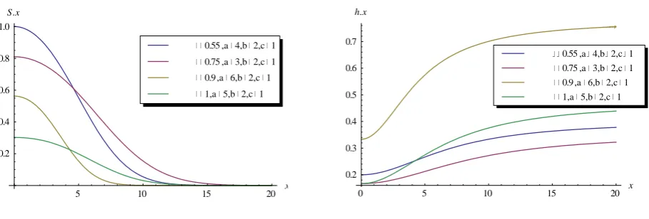
Figure 7: Plots of Survival and Hazard functions for fixed values of with different values of and .
2 4 6 8 10 12 x
0.1 0.2 0.3 0.4 0.5
S.x
0.55 0.75 0.9 1
2 4 6 8 10 12 x
0.6 0.8 1.0 1.2 1.4 1.6
h.x
0.55 0.75 0.9 1
10 20 30 40 50 x
0.1 0.2 0.3 0.4 0.5
S.x
0.55 ,a 6 0.55 ,a 5 0.55 ,a 4 0.55 ,a 3
10 20 30 40 50 x
0.1 0.2 0.3 0.4
h.x
0.55 ,a 6 0.55 ,a 5 0.55 ,a 4 0.55 ,a 3
5 10 15 20 x
0.2 0.4 0.6 0.8 1.0
S.x
1,a 5,b 2,c 1 0.9 ,a 6,b 2,c 1 0.75 ,a 3,b 2,c 1 0.55 ,a 4,b 2,c 1
0 5 10 15 20 x
0.2 0.3 0.4 0.5 0.6 0.7
h.x
From above Figures, it is observed that hazard unction is concave increasing for ( ) except for , at this point, hazard function convex decreases.
4.
Properties
In this section, some Mathematical properties of the LGSE distribution containing moments, moment generating function, cumulant generating function and information entropy.
4.1. Moments, Moment Generating Function
For the moments of the LGSE distribution, the rth moment of Lindley Generalized Stretched Exponential variable with pdf (3) is obtained as:
By definition,
( )
∫ ( )
By substituting right hand side expression of ( )in above expression, we obtain
( ) ( ) ∫ {( ) }
( ) [ {( ) } ] {( ) } (14)
Now suppose that
{( ) }
OR (15)
{( ) }
This implies
{( ) ⁄ }
⁄
{( ) ⁄ }
( ) (16)
Equation (14) can be written as:
( )∫ [ {( ) ⁄
} ⁄
] {( ) }
[{( ) ⁄} ⁄
]
* +
{( ) ⁄
}
After simplification and using Gamma function, ( ) ∫ , we obtain rth moment of LGSE distribution.
⁄ ( )* ( ) ( )+
(17)
For Mean and Variance of X, by putting in Equation (17), the expressions of ( )and ( )aregiven by
( ) ⁄
( )[ ( ) ( )]
(18)
( ) ⁄
( )[ ( ) ( )]
(19) Now Variance of X is obtained by
( ) ( ) [ ( )]
(20) By putting expressions of ( )and ( )in (20), we obtain
( ) ⁄
( )[ ( ) ( )] [ ⁄ ( )[ ( ) ( )]]
OR
( ) ⁄
( )[ ( ) ( ) ( ){ ( ) ( )}]
(21)
The moment generating function (m.g.f) and cumulant generating function (c.g.f) are expressed in the form
( ) ∑ * ⁄ ( ), ( ) ( )-+,
(22)
( ) [∑
[ ⁄
( ), ( ) ( )-]]
(23)
Note: We can also obtain mean and variance of LGSE distribution with help of m.g.f. (22) by using partial differentiation of m.g.f. with respect to t, then substituting , we obtain mean (18), similarly, again applying partial differentiation of m.g.f. with respect to t, then substituting , we obtain ( ) that is used to find variance.
4.2
Information Entropy:
The concept of entropy is significant in various fields of Science, specifically Physics, Theory of communication and Probability.
4.2.1 Renyi’ Entropy
The Renyi entropy for the Lindley Stretched Exponential distribution has been obtained as: Let be the LGSE r.v, then the Renyi’ entropy can be obtained by using the following relation.
( ́)
́ {∫ ́( ) }
(24)
Here ́( ) [
( ){( ) }
( ) [ {( ) } ] {( ) } ]
́
by substituting
the value of ́( ) in equation (19), In process of integration of ́( ) we adopt substitution
method from Equations (15) and (16), then after simplification, we obtain required Renyi’ entropy as given below:
( ́)
́ {
́ ́ ́
́ ( ) ́∑ ( ́) ( ́
́
)
}
(25)
Note: Another type of entropy i.e. Shannon entropy for LGSE distribution can be obtained by using: [ ( )] ∫ [ ( )] ( ) (26)
5.
Maximum Likelihood Estimation
Let be a random sample of size from the LGSE distribution given by equation (3). Then
( ) ∏ ( )
Here, ( ) (27)
By substituting right hand expression of ( ) in (27), applying on both
sides, then we obtain the following result
( ) ( ) ( ) ( ) ( ) ( ) ( ) ( ) ( )∑ ( ) ( )∑ ( ) ∑ [ {( ) }] ∑ {( ) }
(28) By partially differentiation to equation (28) with respect to , we obtain
the following equations in the form of
( ) ( ) ( ) ∑ ( ) (( ) ) ∑ ( ) {( ) } [ {( ) } ]
(29)
( ) ∑ ( ) ( ) ∑ ( ) ∑ ( ) {( ) } ∑ ( ) {( ) } {( ) }
(30)
( ) ∑ ( ) ∑ ( ) {( ) } ∑ ( ) {( ) } {( ) }
(31)
( ) ∑ ( ) {( ) } {( ) }
It have seen that above equations (29), (30), (31) and (32) do not give the impression to be resolved directly. Conversely, Fisher’s scoring method can be used to solve these equations iteratively.
The MLEs ( ̂ ̂ ̂ ̂) of the parameters of LGSED are the solution of the following equations: [ ( ) ( ) ( ) ( ) ( ) ( ) ( ) ( ) ( ) ( ) ( ) ( ) ( ) ( ) ( ) ( ) ] ̂ ̂ ̂ ̂ [ ̂ ̂ ̂ ̂ ] [ ( ) ( ) ( ) ( ) ] ̂ ̂ ̂ ̂
where are initial values of These equations are solved iteratively till sufficiently close estimates of ̂ ̂ ̂ ̂ are obtained. In this connection, Mathematica-software can also be used.
6.
Applications
The Lindley Generalized Stretched Exponential distribution of three parameters has been applied to some real life data- sets due to make a comparison with other models. Because, In this section, we explore the fitting of three and two-parameter Lindley Stretched Exponential distribution to four real life data-sets and make a comparison of its goodness of fit with other distributions including its Special cases, Weibull, Gamma, Lognormal, Generalized Lindley, Generalized Gamma, LG the one parameter Lindley distributions. In order to compare distributions, , AIC (Akaike Information Criterion), CAIC (Consistent Akaike Information Criterion), BIC (Bayesian Information Criterion), HQIC (Hannan Quinn Information Criteria), K-S Statistics (Kolmogorov-Smirnov Statistics) for real life data sets have been computed by using R software.
Note that: The smaller measures of goodness-of-fit provide better the fit of the data. These measures of goodness-of-fit are defined as:
( )
( ( ))
Data 1:
The data set represents an uncensored data set corresponding to remission times (in months) of a random sample of 128 bladder cancer patients reported in Lee and Wang (2003): The remission times (in months) of bladder cancer patients data is given below:
0.08 2.09 3.48 4.87 6.94 8.66 13.11 23.63 0.20 2.23 0.52 4.98 6.97 9.02 13.29 0.40 2.26 3.57 5.06 7.09 0.82 0.51 2.54 3.70 5.17 7.28 9.74 14.76 26.31 0.81 0.62 3.82 5.32 7.32 10.06 14.77 32.15 2.64 3.88 5.32 0.39 10.34 14.83 34.26 0.90 2.69 4.18 5.34 7.59 10.66 0.96 36.66 1.05 2.69 4.23 5.41 7.62 10.75 16.62 43.01 0.19 2.75 4.26 5.41 7.63 17.12 46.12 1.26 2.83 4.33 0.66 11.25 17.14 79.05 1.35 2.87 5.62 7.87 11.64 17.36 0.40 3.02 4.34 5.71 7.93 11.79 18.10 1.46 4.40 5.85 0.26 11.98 19.13 1.76 3.25 4.50 6.25 8.37 12.02 2.02 0.31 4.51 6.54 8.53 12.03 20.28 2.02 3.36 6.76 12.07 0.73 2.07 3.36 6.93 8.65 12.63 22.69 5.49
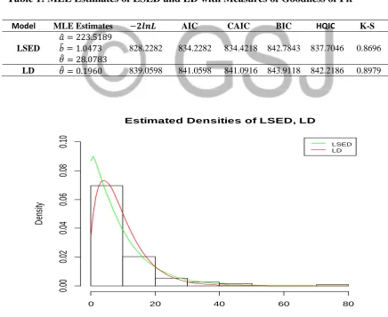
Table 1: MLE Estimates ofLSED and LD with Measures of Goodness of Fit
Figure 8 : Fitted Density curves with remission on times of bladder cancer patients data Estimated Densities of LSED, LD
The remission times (in months) of bladder cancer patients
D
en
si
ty
0 20 40 60 80
0.
00
0.
02
0.
04
0.
06
0.
08
0.
10 LSED
LD
Model MLE Estimates AIC CAIC BIC HQIC K-S
LSED
̂ ̂ ̂
828.2282 834.2282 834.4218 842.7843 837.7046 0.8696
From Table 2 Figure 9, numerically and graphically, it is observed that, LSED gave better performance than LD due to its minimum measures of AIC, CAIC, BIC and HQIC.
Data 2:
The dataset is taken from Gross and Clark (1975, p. 105) and shows the relief times of 20 patients receiving an analgesic. The data are presented below. We fit the LSED, GD, WD and LG distributions to the real dataset.
1.1 1.4 1.3 1.7 1.9
1.8 1.6 2.2 1.7 2.7
4.1 1.8 1.5 1.2 1.4
3.0 1.7 2.3 1.6 2.0
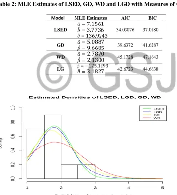
Table 2: MLE Estimates ofLSED, GD, WD and LGD with Measures of Goodness of Fit
Figure 9 : Fitted Density curves with relief time of twenty patients data
Estimated Densities of LSED, LGD, GD, WD
Relief times of twenty patients data
De
nsi
ty
1 2 3 4 5
0.
0
0.
2
0.
4
0.
6
0.
8
1.
0
LSED LGD GD WD
Model MLE Estimates AIC BIC
LSED ̂
̂
̂
34.03076 37.0180
GD ̂
̂ 39.6372 41.6287
WD ̂ ̂
45.1728 47.1643
LG ̂ ̂
From Table 3 Figure 10, numerically and graphically, it is also observed that, LSED gave better performance than LGD, GD, and WD due to its minimum measures of AIC and BIC.
Conclusion:
In this paper the Lindley Generalized Stretched Exponential distribution has been introduced. Its mathematical properties have been derived. The method of Maximum Likelihood has been used to estimate its parameters. The usefulness of distribution has also been shown by four real life data sets. It has been observed from both of results, numerically and graphically that Lindley Generalized Stretched Exponential distribution of three parameters proves a better fit for data connected to all real life data as compared to its specific cases as well as other competitive models.
References
Adamidis K., and Loukas S.,(1998) A lifetime distribution with decreasing failure rate,
Statistics and Probability Letters, 39, 35-42.
Bakouch H. S., Al-Zahrani B. M., Al-Shomrani A. A., Marchi V. A., and Louzada F.,(2012) An extended LD, Journal of the Korean Statistical Society, 41, 75-85.
Ghitany M. E., Alqallaf F., Al-Mutairi D. K., and Husain H. A., (2011) A two-parameter weighted Lindley distribution and its applications to survival data. Mathematics and Computers in Simulation, 81, 1190-1201.
Ghitany M. E., Alqallaf F., Al-Mutairi D. K., and Husain H. A., (2011) A two parameter weighted Lindley distribution and its applications to survival data, Mathematics and Computers in Simulation, 81, 1190-1201.
Gross, A. J. and Clark, V. A. (1975). Survival Distributions: Reliability Applications in the Biomedical Sciences. New York: John Wiley and Sons.
Lawless J. F., (2003) Statistical models and methods for lifetime data. Wiley, New York. Lee E.T. and Wang J.W.,(2003) Statistical Methods for Survival Data Analysis, 3rd
ed.,Wiley, NewYork.
Laherr`ere, J. and Sornette, D. (1998). Stretched exponential distributions in nature and economy: ”fat tails” with characteristic scales. Eur. Phys. J. B 2, 525–539.
Lindley D. V.,(1958) Fiducial distributions and Bayes theorem, Journal of the Royal Statistical Society, Series B (Methodological), 102-107.
Louzada, F., Roman, M., & Cancho, V. G. (2011). The complementary exponential geometric distribution: model, properties, and a comparison with its counterpart.
Mahmoudi E., and Zakerzadeh H., (2010) Generalized Poisson Lindley , Communications in Statistics: Theory and Methods, 39, 1785-1798.
Merovci, F., and Elbatal, I. (2014) Transmuted Lindley-Geometric Distribution and its Applications. Journal of Statistics Applications and Probability, 3, 77-91 (20). Min Wang, (2013) A new three-parameter lifetime distribution and associated inference, MI
49931, USA. http://arxiv.org/abs/1308.4128v1
Sankaran,M.(1970).ThediscretePoisson–Lindleydistribution.Biometrics,26,145–149.
Shanker R., Sharma S., and Shanker R., (2013) A Two-Parameter Lindley for Modeling Waiting and Survival Times Data, Applied Mathematics, 4, 363-368.