Trajectory Tracking Of Wheeled Mobile Robot:
Model-Based Test And Validation Using QBOT
M.Vavuniya, R.Santhiya, A.M.Kirthika, T.SalomiyaPaulin, M.Sivapalanirajan, M.Willjuice Iruthayarajan
Abstract: An important issue in robotics research is trajectory tracking control, where the robot is required to follow a particular path. The error between the desired path and the actual path is to get converged to zero. The problem is more complicated when the robot dynamics is considered. Our Project proposes a real-time trajectory tracking control for a wheeled mobile robot QBOT 2e in both real and model-based simulated environments. The MIMO model of the robot is developed, and it is simulated to test the tendency of the model to track the desired path. The kinematics helps to find the positioning of the robot in the X and Y coordinates. The odometric localization helps to track the path of the Robot. The path planning of the robot from the starting point to the target is developed by using two different algorithms, namely A * Algorithm and the Potential Field Algorithm. The algorithms help to find the robot to calculate the optimized path to reach the target. It is observed that the model is tested and validated with the real benchmark system QBOT.
Index Terms: Wheeled mobile robots, MIMO model, Trajectory tracking, A* algorithms, Potential field algorithm, odometric localization, QBOT.
————————————————————
1
INTRODUCTION
In recent years, there has been enormous activity in the field of robotics. During the past decades, the progress in the class of trajectory tracking of the two-wheeled mobile robot is improved numerously. The main objective of the trajectory tracking is to reach the target without losing the stability of the system [1]. For maintaining the stability of the system, controller design is a crucial part [2]. This is due to the consideration in the kinematic and dynamic model of the robot. Modeling of the Wheeled mobile robot will certainly help to develop the controller. By considering the dynamics of the robot [3], a mathematical model is developed. Another important factor in trajectory tracking is path planning, which can be developed by various algorithms. A* and potential field algorithm are one of the popular algorithm used in path planning [4]. While tracking the trajectory, the path may have obstacles that need to be avoided by the use of sensors is employed [5]. There are a lot of developments by heuristic approaches like the Fuzzy logic controller to control the wheeled mobile robots by using various membership functions [6], [7]. The constraints of the wheeled mobile robot are to be considered in the design of controller and system design, which is termed as non-holonomic and holonomic constraints. The non-holonomic constraint is considered in [8], and the fuzzy controller is used in trajectory tracking [9] to the constraint. Real-time implementation of the robotic system is a crucial part of the trajectory tracking [10]. The real-time system with Lyapunov based controller [11], fuzzy sliding mode [12] are developed for wheeled mobile robots.The QBOT 2e is a benchmark model developed by Quanser [13].
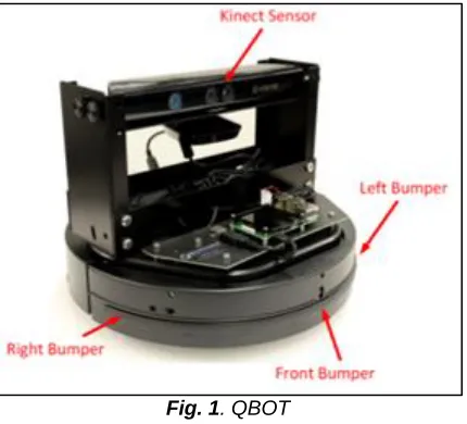
It is an innovative open-architecture autonomous ground robot, equipped with built-in sensors, and a vision system. By extensive applications of the wheeled mobile robot, QBOT 2e is ideally suited for validating the mathematical simulation and control the wheeled mobile robot. It is also useful for teaching undergraduate and advanced robotics and mechatronics courses to correlate the capabilities of robotics [14]. The open-architecture control structure allows the users to add off-the-shelf sensors and customize the QBOT 2e for their research needs. The aim of Robotics in trajectory tracking application is to make the robot to track the desired path and make it ready to track the target location in an optimized way. The QBOT 2e Mobile Platform consists of two central drive wheels mounted is controlled by GA based PID controller [15]. Fuzzy with a PD controller is incorporated for QBOT [16]. This configuration is known as a two-wheeled differential drive robot. Castors are available in the front and back of the robot for stabilizing the platform without compromising its movements. The two drive wheels are independently driven in both forward and backward for actuating the robot wheels. This approach of mobile robot wheel geometry analysis is very common due to its simple and maneuverable nature. The motion of the wheels is measured using an optical encoder, and the robot's orientation or yaw angle, are estimated during the integrated gyro. For more information on the Kinematics of the QBOT 2e and how it can generate wheel commands to achieve specific motion trajectories, refer to the Forward/Inverse kinematics methods. In addition to the encoders and gyro, the QBOT 2e comes with a Microsoft Kinect for vision, shown in Figure 1, that outputs color image frames (RGB) as well as depth information. You can process RGB and depth data for various purposes, including visual inspection, 2D and 3D occupancy grid mapping, visual odometry, etc. The QBOT 2e also comes with integrated bump sensors (left, right, and central) and cliff sensors (left, right, and central). These sensors can be used in a control algorithm to avoid obstacles or prevent damage to the robot. A Cliff Sensor is important to have the systems to avoid excessive drops which damage the robot. Roomba models come with a cliff sensor to help them avoid driving over stairwells or ledges.
________________________________
• Ms.M.Vavuniya is currently pursuing a bachelor degree program in the department of Electrical and Electronics Engineering, National Engineering College(NEC), India, E-mail: [email protected] • Ms.R.Santhiyais currently pursuing a bachelor degree program in the
department of EEE, NEC, India, E-mail:[email protected] • Ms.A.M.Kirthika is currently pursuing a bachelor degree program in the
department of EEE, NEC, India, E-mail:[email protected] • Ms.T.SalomiyaPaulinis currently pursuing a bachelor degree program in
the department of EEE, NEC, India, E-mail: [email protected] • Mr.M.Sivapalanirajan is currently working as Assistant Professor in the
Department of EEE, NEC, India, PH-9578175275. E-mail:
Fig. 1. QBOT
The Microsoft X-Bot Kinetic sensor is a revolutionary new depth camera that is used Robotics to capture the motions of the People and efficiently in Obstacle avoidance using the technology of an RGB camera and infrared camera to differentiate depth.
The bumper sensor detects the collision before it really happens. This sensor works as an SPST switch. When the whisker bumps the foreign object, it will make contact with a nut next to it, closing the connection, and, by default, the motor will be turned off. By attaching these mechanical bumpers to the robot, the whisker will bump before the robot crashes. The sensor has a 3-pin header for connecting the mainboard directly via jumper wires. A Gyro (gyroscope) sensor is used to monitor the robot's direction of movement. It is used to make sure that it travels in a straight line or to control turns accurately. A Gyro sensor reports any directional change by the robot, and that information used to control the direction of travel.
2
MODELING
OF
QBOT
QBOT is a mobile robot which can be modeled as two aspects
● Kinematic modeling
● Dynamic modeling
2.1KINEMATIC MODELING
The kinematic model for the two-wheel differentially driven WMR can be defined using the following relations: Let 𝑣𝑅, 𝑣𝐿, and 𝑣𝐶 be the linear velocities of robot right wheel, left wheel, respectively. Then, the linear velocity of the center of mass,
Vc = (VR+VL)/2. (1)
The angular velocity is given by,
Ɵ̇= (VR−VL)/d (2)
Where d is the distance between the wheels of QBOT 2.
2.2DYNAMIC MODELING
The dynamic modeling of WMR is discussed in this section. It can be derived using Euler-Lagrange formulation:
d/dt ( ∂L/∂q̇i ) − ( ∂L/∂qi ) = Qi (3)
Where L stands for the difference of kinetic energy T and potential energy U, qi stands for generalized coordinate, and Qi stands for a generalized force that acts on the mechanical system. Under the assumption that the mobile robot moves only on a plane surface, the potential energy of the robot is
zero (U = 0), and one has to find only the kinetic energy of the mobile robot. The kinetic energy of the WMR can be determined as the sum of the kinetic energy of mobile robot translation (Tt), the kinetic energy of mobile robot rotation (Tr),
and the kinetic energy of rotating wheels and rotors of DC motor (Trwr). Hence,
𝑇𝑡 = ½(𝑚V𝑐)2 = 1/2m (𝑥𝑐2̇ + 𝑦𝑐2̇) (4) 𝑇r = ½ 𝐼𝑎𝜃̇
2
(5) 𝑇𝑟𝑤𝑟 = 1/2I0𝜃𝑅2̇ + 1/2𝐼0𝜃𝐿2̇ (6)
Then the Lagrange equations become:
d/dt ( ∂T /∂Ɵ̇R ) − ( ∂T /∂ƟR ) = τR (7)
d/dt ( ∂T /∂Ɵ̇L ) − ( ∂T /∂ƟL ) = τL (8)
TABLE1
SPECIFICATION PARAMETERS OF QBOT
The state of the dynamic model for the WMR is chosen as follows: x1 = 𝜃𝑅̇; x2 = 𝜃𝐿̇ ; x3 = iR and x4 = iL, where𝑖𝑅 and 𝑖𝐿are motor currents of the right and left wheel respectively.
The state-space representation of the WMR dynamics is of the form:
ẋ = Ax + Bu. (9)
The transfer function representation of the WMR dynamics can be obtained as G(s) = C (SI − A)−1B with system
parameters in table 1. The G(s) will be in the form of a TFM given as:
(10)
The transient response specifications of practical systems include delay time, rise time, peak time, maximum overshoot, and settling time. The response of WMR is also found to be overdamped. These time-domain specifications of the desired response have been taken into consideration during the design of MIMO's desired closed-loop system. The velocity levels of the WMR don’t attain the steady-state value instantly. Instead, it reaches the steady-state with a finite settling time and exhibits over-damped characteristics. The desired closed-loop system dynamics can be expressed as
(11)
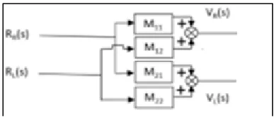
Here, the M(s) represent the MIMO desired closed-loop Transfer function model, VR, and VL is the desired steady-state
Fig. 2. Block diagram of the desired closed-loop system with dynamics
The desired output response can be taken as, 𝑌1(𝑠) = 𝑉𝑅(s) = 𝑅𝑅𝜔𝑛
2
/[𝑠(𝑠2
+2𝜁𝜔𝑛𝑠+𝜔𝑛2)] (12) 𝑌2(𝑠) =𝑉𝐿(𝑠) = (𝑝−1)/(𝑝+1) (13)
Where, p = 2rT/ d. rT is the center of circular trajectory.
The off-diagonal elements of M(s) represents the desired cross-coupling interaction expected to be present in the designed closed-loop system. Hence one can control the cross-coupling effect in the designed closed-loop system by changing the off-diagonal elements in the MIMO desired closed-loop TFM. In the present work, both off-diagonal elements of M(s) is taken as a first-order system with pole location at s = -λ.
𝑀12(𝑠) = 𝑀21(𝑠) = 1/(𝑠+𝜆) (14)
The off-diagonal elements are chosen as a first-order system, described in section 3. In the present work, off-diagonal elements of M(s) are chosen with the degree of interaction, λ = 1000. Then the diagonal elements of the desired closed-loop TFM are obtained as described in Section 3 as:
M11(s)=(−0.5s 2
+9.2231s+13217)/(s3+1008s2+8013s+13223) (15) M22(s) = (−2s
2
−2.7769s+13197)/(s3
+1008s2+8013s+13223) (16)
The damping ratio for desired output response ζ present in the desired output response Y(s) is taken as 1.1. While the desired right and left wheel velocities are taken as RR = 0.2
m/s, RL = 0.1 m/s, and settling time=1s,
Y1(s) = 2.645/(s 3
+8s2+13.22s) (17) Y2(s) = 1.322/(s3+8s2+13.22s) (18)
Figure 3 shows the implemented simulink model of QBOT
Fig. 3. MIMO model of QBOT in Simulink
3
PATH
PLANNING
The Quanser QBOT 2 Mobile Platform comes with a Kinect sensor that has the ability to generate a depth map of the environment. This information, along with the location and orientation of the robot chassis, can be used for autonomous map building. The 2D map generated using this data will be processed to locate various obstacles in the map and create the "occupancy grid map" of the environment. Global path planning methods search for the connected grid components between the robot and the target. Here we use A* and potential field techniques for global path planning.
3.1A*ALGORITHM
A* is one of the most popular choices for path planning because it's fairly simple and flexible. This algorithm considers the map as a two-dimensional grid with each tile being a node or a vertex. A* is based on graph search methods and works by visiting vertices (nodes) in a graph, starting with the current position of the robot all the way to the goal. The significance of the algorithm is identifying the appropriate successor node at each step. Given the information regarding the goal node, the current node, the obstacle nodes, we can make an educated guess to find the best next node and add it to the list. A* uses a heuristic algorithm to guide these arch while ensuring that it will compute a path with minimum cost. A* calculates the distance (also called the cost) between the current location in the workspace, or the current node, and the target location. It then evaluates all the adjacent nodes that are open (i.e., not an obstacle nor already visited) for the expected distance or the heuristic estimated cost from them to the target, also called the heuristic cost, h(n). It also determines the cost to move from the current node to the next node, called the path cost, g(n). Therefore, the total cost to get to the target node, f(n) = h(n) + g(n), is calculated for each successor node, and the node with the smallest cost is chosen as the next point. Using either the path cost g(n) or heuristic cost h(n) exclusively will result in non-optimized paths. Together, an optimized path from the current node to the target node can be achieved. Figure 4 shows how the A* algorithm finds a way between the robot's position and target position. It finds the most optimized way to reach the target.
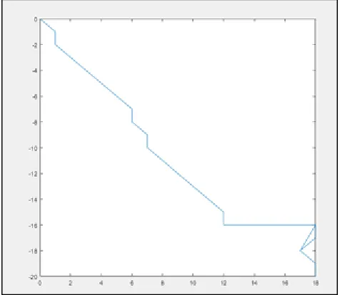
Fig. 5. Position of the robot while moving in A* algorithm
Figure 5 shows the position of the robot from an initial position to the target. The actual X and Y position of the robot is similar to the path generated by the A* algorithm.
3.2POTENTIAL FIELD ALGORITHM
In this approach, the target exhibits an attractive potential field (Utarget), and the obstacles exhibit repulsive potential fields
(Uobsi). The resultant potential field is produced by summing
the attractive and repulsive potential fields as follows. U = Utarget +∑Uobsi (20)
The net potential field is used to produce an artificial force equivalent to the gradient of the potential field with a negative sign as follows.
F = −∇U (21)
The motion is then executed by following the direction of the created force. A common problem of the potential field method is that the robot is trapped in a back-and-forth oscillatory motion when attractive and repulsive forces work in a straight line. Figure 6 shows the generated path using the potential field algorithm. But it does not reach the target position. So we have to stop the robot manually. And the path is more oscillatory in nature, which is given in figure 7.
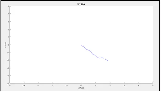
Fig. 6. Path planning using potential field algorithm
Fig. 7. Position of the robot while moving in the potential field algorithm
5
RESULT
AND
DISCUSSION
Figure 8 shows applied velocity Vc to the QBOT. After inverse
kinematics, the Right and left wheel velocity are calculated and applied to the motor through encoders. The input velocity is calculated by the algorithm, and the actual velocity is measured through encoders.
Fig. 8. Chassis velocity input and output for QBOT
Figure 9 shows the applied and measured velocity in and out of the transfer function model. The response shows that the control effort provided by the system is higher when compared to the actual system.
The trajectory tracking performance of the QBOT system for the A* algorithm is shown in figure 10, which indicated the tracking of the real system model to the desired task.
Fig. 10. The response of QBOT with A* algorithm
Similarly, figure 11 shows the response of QBOT for potential field algorithm, which indicates less effort, and there is no sharp change in trajectory guidance and tracking.
Fig. 11.The response of QBOT with potential field algorithm
The same planning data input is used to test the response of the developed MIMO model as Simulink. The response tracks the actual system response shown in table 2.
Fig. 12.The response of the MIMO model with A* algorithm
Fig. 13.The response of the MIMO model with Potential field algorithm
Figure 12 tracks the desired trajectory provided by A* algorithm with considerably less error than potential field input data to the MIMO model shown in figure 13. Both X and Y-axis coordinates are distance in centimeter.
TABLE2
PERFORMANCE COMPARISON QBOT AND MIMO MODEL
From table 2, performance measures are listed with Vc as the
chassis velocity in m/S, peak time Tp in seconds and Settling
time, Ts in seconds The performance parameters shows that
the path planning algorithms ability to take the robot from starting point to destination point. A* algorithm tracks the destination with minimum effort and takes slightly higher time for reaching the destination. The potential field algorithm has a faster settling time, but it consumes higher control effort and improper destination tracking. The real experimental validation setup is shown in figure 14.
Parameters
A* ALGORITHM POTENTIAL FIELD ALGORITHM
QBOT MIMO
MODEL QBOT
MIMO MODEL VC (m/S) 0.415 0.425 0.338 0.347
Tp (Sec) 8.32 4.30 16.75 11.96
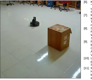
Fig. 14.Experimental Validation
6
CONCLUSION
From the response of the system model and QBOT real-time response, it is inferred that the model is capable of imitating the system response with considerably less error of 0.1cm tolerance. Odometric localization inferred the current location of the robot in Cartesian space. The path planning algorithm A* is comparatively efficient than the potential field algorithm in terms of minimum control effort and perfect tracking. The response graph shows that the model recreates the real system response for both A* and Potential field algorithm. The overall tracking performance of the system can be improved further by adopting various control structures. The proposed MIMO system can be utilized in the design of the controller and its analysis to study the response of real system with the model.
7
REFERENCES
[1]. Huang, L. and Tang, L., "Dynamic target tracking control for a wheeled mobile robot constrained by limited inputs." IFAC Proceedings Vol: 41(2), pp.3087-3091, 2008. [2]. R.Rajagopalan, N.Barakat ―Velocity Control of Wheeled
Mobile Robots Using Computed Torque Control and Its Performance for a Differentially Driven Robot," Journal of Robotic systems Vol. 14(4), pp. 325-340, 1997
[3]. EdouardIvanjko, Toni Petrinić, and Ivan Petrović. 2010. "Modelling of mobile robot dynamics." 7th EUROSIM Congress on Modelling and Simulation, Sep. 6-10), 2010.
[4]. Duchoň, František, et al. "Path planning with modified a star algorithm for a mobile robot." Procedia Engineering 96 (2014): 59-69.
[5]. Bellur Ravindra, Vibha. ―Real-time Path Planning and Obstacle Avoidance for Mobile Robots with Actuator Fault," Theses and Dissertations 2019, Wright State University.
[6]. K. N. Faress, M. T. El Hagry, and A. A. El Kosy, "Trajectory tracking control for a wheeled mobile robot using fuzzy logic controller," WSEAS Transactions on Systems, 4(7):1017–1021, 2005.
[7]. M. Yang and J.-H. Kim, Sliding mode control for trajectory tracking of non-holonomic wheeled mobile robots, IEEE Transactions on Robotics and Automation, 1999 vol. 15, no. 3, pp.578-587.
[8]. Sanhoury, Ibrahim MH, Shamsudin HM Amin, and Abdul Rashid Husain. "Tracking Control of a Non-holonomic Wheeled Mobile Robot." 2012, PIM Volume1 issue 1, pp. 7-11.
[9]. Falsafi, Mohammad Hossein, Khalil Alipour, and BahramTarvirdizadeh. "Tracking-Error Fuzzy-Based Control for Nonholonomic Wheeled Robots." published in Arabian Journal for Science and Engineering in 2019, Vol. 44, issue 2, pp. 881-892.
[10]. Lee, T. H., et al. "A practical fuzzy logic controller for the path tracking of wheeled mobile robots." IEEE Control Systems Magazine Vol.23 issue 2, pp.60-65.
[11]. Mohammed Elsayed, Abdallah Hammad, Ashraf Hafez, Hala Mansour, ―Real time Trajectory tracking controller based on Lyapunov function for mobile robot" published in the International Journal of Computer Applications in 2017, Vol:168 No.11, pp.-1-6.
[12]. Wu, Xing, et al. "Backstepping Trajectory Tracking Based on Fuzzy Sliding Mode Control for Differential Mobile Robots." Journal of Intelligent & Robotic Systems, 2019, pp: 1-13.
[13]. Amir Haddadi, Peter Martin, and Cameron Fulford.Quanser QBOT 2 Complete Workbook (Instructor). Quanser, Canada. 2015.
[14]. Rajibul Huq, Herv´e Lacheray, Cameron Fulford, Derek Wight, and Jacob Apkarian, "QBOT: An Educational Mobile Robot Controlled In Matlab Simulink Environment." Canadian Conference on Electrical and Computer Engineering. IEEE, 2009.
[15]. Damodaran Suraj, T. K. Kumar, and Attadappa Puthanveetil Sudheer, "Design and implementation of GA tuned PID controller for desired interaction and trajectory tracking of wheeled mobile robot," Proceedings of the Advances in Robotics, ACM, 2017.