https://doi.org/10.5194/ascmo-5-67-2019 © Author(s) 2019. This work is distributed under the Creative Commons Attribution 4.0 License.
Comparison and assessment of large-scale surface
temperature in climate model simulations
Raquel Barata, Raquel Prado, and Bruno Sansó
Department of Statistics, University of California Santa Cruz, Santa Cruz, CA 95064, USA
Correspondence:Raquel Barata ([email protected])
Received: 13 August 2018 – Revised: 29 April 2019 – Accepted: 3 May 2019 – Published: 27 May 2019
Abstract. We present a data-driven approach to assess and compare the behavior of large-scale spatial averages of surface temperature in climate model simulations and in observational products. We rely on univariate and multivariate dynamic linear model (DLM) techniques to estimate both long-term and seasonal changes in tem-perature. The residuals from the DLM analyses capture the internal variability of the climate system and exhibit complex temporal autocorrelation structure. To characterize this internal variability, we explore the structure of these residuals using univariate and multivariate autoregressive (AR) models. As a proof of concept that can easily be extended to other climate models, we apply our approach to one particular climate model (MIROC5). Our results illustrate model versus data differences in both long-term and seasonal changes in temperature. De-spite differences in the underlying factors contributing to variability, the different types of simulation yield very similar spectral estimates of internal temperature variability. In general, we find that there is no evidence that the MIROC5 model systematically underestimates the amplitude of observed surface temperature variability on multi-decadal timescales – a finding that has considerable relevance regarding efforts to identify anthropogenic “fingerprints” in observational surface temperature data. Our methodology and results present a novel approach to obtaining data-driven estimates of climate variability for purposes of model evaluation.
1 Introduction
Exploring the impacts of anthropogenic climate change is of great relevance and interest to society. Phase 5 of the Coupled Model Intercomparison Project (CMIP5) generated many different ensembles of climate model simulations (Tay-lor et al., 2012). These simulations have enhanced our scien-tific understanding of the ability of current models to rep-resent key features of prep-resent-day climate. They have also helped to identify human and natural influences on historical climate and to quantify uncertainties in projections of future climate change. The CMIP5 framework incorporates results from large multi-model ensembles, and frequently includes multiple realizations for each model and type of simulation. More extensive details of the CMIP5 experimental design are found in Taylor (2009).
In this paper we present a statistical model-based ap-proach to compare the observational record with three differ-ent types of CMIP5 simulations. We seek to develop a con-sistently principled way of determining whether there are
sta-tistically significant differences in aspects of the variability, both between the model simulations and the observational record, and within three different types of simulation. Our primary goal is to illustrate the utility of Bayesian statistical techniques that are not in widespread use in climate science. We develop a data-driven model diagnostic method and pro-tocol with potential application to future CMIP model evalu-ation.
tem-perature time series is statistically principled and consistent across different series, and the results incorporate probabilis-tic uncertainty as the approach is model-based.
To illustrate our statistical methods, we focus on one spe-cific climate model: version 5 of the atmosphere–ocean gen-eral circulation model (AOGCM), which has been jointly developed by the Atmosphere and Ocean Research Insti-tute at the University of Tokyo, the National InstiInsti-tute for Environmental Studies, and the Japan Agency for Marine-Earth Science and Technology (see Watanabe et al., 2010). From this model, commonly referred to as the Model for Interdisciplinary Research on Climate (MIROC5), we ex-amine three different types of simulations: (1) decadal pre-dictions of climate, initialized from a specific observational state; (2) uninitialized simulations driven by estimated histor-ical changes in key anthropogenic and natural forcings; and (3) control integrations with no year-to-year changes in ex-ternal forcings, which provide estimates of the natural inter-nal variability of the climate system. Our ainter-nalysis focuses on monthly mean 2 m surface temperature time series over four regions: global, tropical, Northern Hemisphere and Southern Hemisphere. This allows us to explore the sensitivity of our results to spatial differences in the large-scale structure of the “signal” (the climate response to imposed changes in exter-nal forcings) and the “noise” of natural interexter-nal variability. Our statistical analysis of MIROC5 simulations can be easily extended to other models in the CMIP archive.
Our approach extracts long-term externally forced changes in temperature, seasonality and estimates of internal variabil-ity of the climate model simulations and compares them to the corresponding components in observational products. As in Imbers et al. (2014), our focus is on investigating the spec-tral characteristics of internal variability. We seek to deter-mine whether model versus observed spectral differences are significant, and can be interpreted in terms of known model deficiencies (such as systematic errors in external forcings; see Solomon et al., 2011; Schmidt et al., 2014). Addition-ally, we investigate whether there are identifiable differences between the spectral properties in the decadal prediction, his-torical, and control simulations that are related to factors such as the inclusion of external forcings and the initialization ap-proach.
The paper is organized as follows. In Sect. 2, we describe the model simulations and the observational products ana-lyzed here. Section 3 presents our statistical modeling ap-proach and introduces the DLM used to estimate the base-line and seasonal components of the time series. Section 3 also describes the AR model that we apply to the residual time series in order to estimate natural internal variability. In Sect. 4, we show the results obtained from the application of the DLM and AR models to the surface temperature time se-ries for the four regions previously mentioned in a short-term analysis (30 years). Section 5 presents results obtained simi-larly for a long-term analysis (63 years). Section 6 provides a summary and brief discussion.
2 Data
2.1 Climate model simulations
CMIP5 is a coordinated international modeling activity in-volving a large suite of simulations performed with several dozen different climate models. As this study is primarily an exposition of methodology rather than a comprehensive anal-ysis of internal variability behavior in CMIP5 models, we fo-cus here on simulations performed with one particular state-of-the-art climate model (MIROC5). We analyze both forced and unforced climate simulations. The forced decadal pre-diction and historical runs are used to explore the response of the climate system to specified historical changes in anthro-pogenic and natural external factors. Examples of such ex-ternal factors include anthropogenic changes in well-mixed greenhouse gases and natural changes in volcanic aerosols (Kirtman et al., 2013). For a full description of the charac-teristics of the different CMIP5 simulations, see Van Vuuren et al. (2011). The forced simulations also reflect the natu-ral internal variability of the climate system. In contrast, the MIROC5 control integration yields an estimate of “pure” nat-ural internal variability, uncontaminated by externally forced climate changes. Below, we briefly describe the three types of climate simulation that are of interest here.
Decadal prediction simulations are the newest addition to the CMIP activity, and are therefore the most exploratory. These near-term simulations were organized through a collaboration between the World Climate Research Pro-gramme’s Working Group on Coupled Modeling (WGCM) and the Working Group on Seasonal to Interannual Predic-tion (WGSIP). There are two core sets of these near-term experiments. The first is a set of 10-year hindcasts initial-ized from a number of different observational starting points. Such simulations allow analysts to assess the prediction skill and to investigate the sensitivity of skill to differences in the initial state (e.g., to the presence or absence of a volcanic eruption or a strong El Niño or La Niña). The second set of decadal prediction runs extended the 10-year hindcasts to 30 years. The influence of external forcing is more promi-nent in these longer simulations (Taylor et al., 2012). The period from 1981 to 2010 is one of the few periods for which 30-year-long decadal simulations are available. This dictates the time period and the length of our short-term analysis. It also explains the absence of decadal simulations in our long-term analysis, which spans the period from 1950 to 2012. The decadal prediction runs include the same time-varying anthropogenic and natural external forcings that are used in the historical simulations.
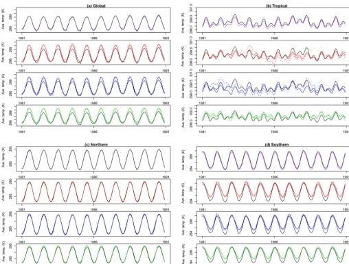
Figure 1.The 10-year series of monthly mean, spatially averaged 2 m surface temperature from the MIROC5 model. The top plots in each panel correspond to NCEP-2 and ERA-Interim reanalyses. The three remaining plots in each panel correspond to the three different types of simulations, in vertical descending order, decadal, historical, and control (labeled “M-” for model in the header). Three realizations of each model simulation are indicated by different line types. The top panels represent global(a)and tropical(b)regions; the bottom panels represent the Northern Hemisphere(c)and Southern Hemisphere(d).
Six individual realizations of the MIROC5 decadal pre-diction run were available (see Fig. 1). Each realization has small differences in the initial state in 1981. These small ini-tial differences amplify with time, eventually yielding differ-ent sequences of natural internal variability in each realiza-tion (Kirtman et al., 2013).
Historical runs are not initialized from a specific observed three-dimensional ocean state. Such simulations typically commence from estimated atmospheric greenhouse gas lev-els in 1850 or 1860, and are then run until the early 21st cen-tury. Like the decadal simulations, the historical simulations are driven by estimated changes in well-mixed greenhouse gases, particulate pollution, land surface properties, solar ir-radiance, and volcanic aerosols. The MIROC5 historical
in-tegrations span the period from 1850 to 2012; five historical realizations were available.
The longest period of overlap between the MIROC5 decadal and historical runs is from January 1981 to Decem-ber 2010 (see Fig. 1). This is the period of our short-term analysis. Our long-term analysis over January 1950 to De-cember 2012 allows us to explore the sensitivity of model versus data comparisons to the use of a longer record (and hence provides a stronger observational constraint on decadal variability).
pre-diction runs are related to the initialization of the latter. Ini-tialization forces the model ocean temperature and sea ice to be consistent with the estimated observational state in 1981. No such consistency with observations is imposed in the his-torical run. Therefore, the two types of simulation can pro-duce noticeably different climate states in 1981. This differ-ence is due to two factors. First, any systematic model errors (in either the applied forcings and/or the climate response to these forcings) should begin to manifest within 1–2 years of the start of the historical run in 1850, causing the simu-lated climate in the historical run to drift away from observed climate. Second, even if there were no model forcing or re-sponse errors, the phasing of internal variability is different in the historical and decadal prediction runs – so the mean states of these two types of simulation are unlikely to be ex-actly the same in 1981 (except by chance).
Control simulations provide estimates of “pure” internal variability, which is an integral component of climate change detection and attribution studies (Santer et al., 2018). In the MIROC5 pre-industrial control simulation analyzed here, there are no year-to-year changes in the atmospheric con-centrations of greenhouse gases, particulate pollution, vol-canic aerosols, or solar irradiance. Changes in climate arise solely from the behavior of modes of variability intrinsic to the coupled atmosphere–ocean–sea-ice system. Examples of such modes of variability include the El Niño–Southern Os-cillation (ENSO), the Interdecadal Pacific OsOs-cillation (IPO), and the North Atlantic Oscillation (NAO). Control runs are typically used to simulate many centuries of internal vari-ability and do not have any direct correspondence with ac-tual time. To create compatibility with the record length of the data available for other simulation runs, we extract 10 nonoverlapping monthly mean temperature time series from the 670-year MIROC5 control run. In the short-term analysis, we extract ten 30-year time series. For the long-term anal-ysis, ten 63-year time series are extracted from the control run. Each 30-year (or 63-year) segment contains a different unique manifestation of internal variability, so they are simi-lar to the realizations available for the decadal prediction and historical runs and we regard them as such (see Fig. 1).
Several points should be emphasized prior to the discus-sion of the model results. First, the AOGCM simulations analyzed here generate their own intrinsic variability – i.e., they produce their own sequences of El Niños, La Niñas, and other quasi-periodic modes. In the historical runs, there is no correspondence between the modeled and observed phas-ing and amplitude of these modes, except by chance. In the decadal prediction runs, the situation is different. The obser-vational ocean data used in the initialization provide some in-formation about the current state of ENSO and other, longer-timescale modes of variability. This observational informa-tion constrains (at least in the first 1–2 years after initializa-tion) the climate trajectory that is followed in the decadal prediction run, imparting some short-term similarity between the simulation and observations. As the length of time
af-ter initialization increases, chaotic variability begins to over-whelm the information that the initialization provided about the likely trajectories of real-world modes of internal vari-ability, and the phasing of internal variability begins to di-verge in observations and the decadal prediction runs.
Second, the observational record, the historical runs, and the decadal prediction simulations contain common com-ponents of temperature variability associated with natural changes in solar irradiance and volcanic activity. For the 30-year period of interest (January 1981 to December 2010), the main solar forcing of interest is the roughly 11-year solar cy-cle (Kopp and Lean, 2011). The major volcanic eruptions are those of El Chichón in 1982 and Pinatubo in 1991. Both erup-tions produced short-term (1–2 year) cooling of the Earth’s surface, followed by gradual recovery to pre-eruption tem-perature levels (Santer et al., 2001). As noted above, the con-trol simulation does not include any solar or volcanic forcing, so each control segment should not exhibit any synchronic-ity between the simulated and observed temperature variabil-ity (except by chance). Further details of the MIROC5 model and the simulations performed with it can be found in Watan-abe et al. (2010).
2.2 Observational records
We compare the climate model simulations to reanalysis ob-servational products and to one in situ obob-servational record. Reanalyses rely on a state-of-the-art numerical weather pre-diction (NWP) model to produce internally and physically consistent estimates of changes in real-world climate. The NWP model assimilates raw observational data from satel-lites, radiosondes, aircraft, land surface measurements, and many other sources, and produces an optimal “blend” of the assimilated data. A key point is that reanalyses are retro-spective – the forecast model does not change over time, so the reanalysis output is not contaminated by spurious changes in climate associated with progressive improvement of the forecast model, or by changes over time to the as-similation system. A number of different groups around the world have generated reanalysis-based estimates of histori-cal climate change. Each group uses a different NWP model and assimilation system and makes different subjective judg-ments regarding the types of observations that are assimi-lated, the weights applied to each data type, and the bias cor-rection procedures applied to the ingested observations. This leads to differences in the estimates of “observed” climate change and climate variability generated by different reanal-ysis products (Kalnay et al., 1996). These differences have generally decreased over time, as NWP models and assimi-lation methods have improved.
NCEP-2 spans the longer period from 1979 to NCEP-2016. Further de-tails of NCEP-2 are available in Kanamitsu et al. (2002). The second reanalysis was generated by the European Centre for Medium-Range Weather Forecasts (ECMWF) in collabora-tion with a number of other institucollabora-tions. We subsequently re-fer to this reanalysis as ERA-Interim (ERA-I). It begins in 1979 and is continuously updated. Results from both reanal-yses are shown in Fig. 1. For a detailed documentation of ERA-I, see Berrisford et al. (2011) and Dee et al. (2011). A more thorough discussion and comparison of these reanaly-ses is available in Fujiwara et al. (2017).
We rely on two observational records for our long-term analysis. The first is the ensemble mean of the 20th Cen-tury Reanalysis Version 2 (20CRV2) observational prod-uct. This reanalysis was jointly performed by the National Oceanic and Atmospheric Administration (NOAA) and the Cooperative Institute for Research in Environmental Sci-ences (CIRES) at the University of Colorado. The 20CRV2 reanalysis does not assimilate any upper-air information from radiosondes and satellites – it only incorporates surface ob-servations of synoptic pressure, monthly sea surface temper-ature, and sea ice distribution (Compo et al., 2011). Inclu-sion of a reanalysis that has fewer sources of input data in our analysis potentially provides a more homogeneous sur-face temperature record. Further details on the 20CRV2 re-analysis can be found in Compo et al. (2011). The second observational record in our long-term analysis is the in situ observational record from the Berkeley Earth Surface Tem-perature project (BEST). Gridded monthly mean temTem-perature fields were generated using an averaging process described in Rohde et al. (2013). Results are for land and ocean tem-perature and for air temtem-perature over sea ice. BEST data are available from 1850 to the present, although we only con-sider data from January 1950 until December 2012. Note that observational products before the satellite era, which began around 1979, are subject to regions with limited in situ data. The choice of time period for the long-term analysis is mo-tivated by surface temperature coverage being degraded in the first half of the century and problems with sea surface temperature (SST) measurements at the time of the Second World War. Further details on the data and BEST averaging process can be found in Rohde et al. (2013).
All model and observational surface temperature data are available in gridded form for a global domain. We calculate area-weighted spatial averages over four regions: the globe (90◦S to 90◦N), the tropics (20◦S to 20◦N), the North-ern Hemisphere (0 to 90◦N), and the Southern Hemisphere (90◦S to 0◦). As an example of the data considered here, we show the first 10 years of the three different types of sim-ulation analyzed in Fig. 1. Globally averaged temperature exhibits a pronounced annual cycle which is clearly dom-inated by the Northern Hemisphere. As expected based on the changes in incoming solar radiation as a function of lat-itude and season, the phasing of the annual cycle differs in the Northern and Southern hemispheres. A semiannual cycle
is apparent in the tropics (Santer et al., 2018). Our statistical analyses focus on these area-averaged time series.
3 Statistical models for model-generated and
reanalysis time series
The protocol presented in this section involves decomposing each temperature time series into what we refer to as a “base-line” and a seasonal component using dynamic linear models (DLMs). The baseline component aims to capture long-term externally forced changes in temperature, whereas the sea-sonal component is dominated by the externally forced an-nual and semianan-nual cycles. We extract the baseline temper-ature and seasonality of the climate model simulations and seek to compare them to the corresponding components in the observational products. The DLM residuals, which have the baseline and seasonal components of the temperature re-moved, are time series that primarily represent natural in-ternal climate variability. Using autoregressive (AR) models, we investigate the spectral characteristics of internal variabil-ity both between the simulations and observational products, as well as within the simulated experiments.
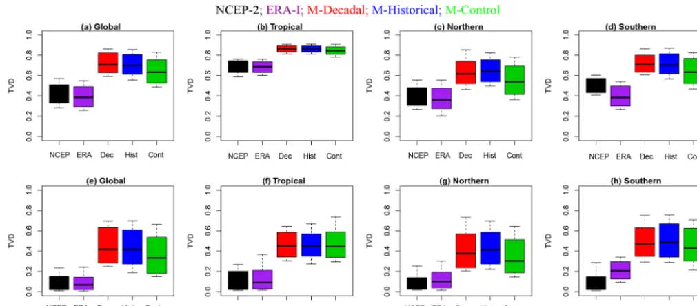
DLMs are a popular Bayesian modeling approach for the analysis of nonstationary time series. We follow approaches detailed in West and Harrison (1999) and Prado and West (2010) in order to estimate time-varying baseline and sea-sonality components. One of the main advantages of using DLMs is that they naturally deal with nonstationary data and allow us to extract the baseline and seasonality com-ponents jointly, while quantifying the uncertainty associated with each component. In Sect. 3.1, we present the DLM used here to extract the baseline and seasonal components from the spatially averaged model and observational surface tem-perature time series. Section 3.2 details the multivariate ex-tensions of the univariate analysis that are required to deal with the availability of multiple realizations of the model simulations. Section 3.3 presents our DLM discount factor selection strategy. Section 3.4 describes a Bayesian approach to fitting autoregressive models to investigate the DLM resid-uals and their spectral properties. Section 3.5 presents the re-sults of using the total variation distance (TVD) as a method to compare the spectra of the DLM residuals. Section 3.6 concludes with a summary of our complete data analysis pro-tocol.
3.1 Baseline and seasonal temperature estimation Consider first a single observational product time series for one of the four domains considered. Letyt denote the
univariate domain-average temperature at time t, for t= 1, . . ., T where T is 360 months for the short-term analy-sis (30 years) and 756 months for the long-term analyanaly-sis (63 years). We decompose each time series into a baseline temperatureη1,t and seasonal componentsα1k,t for
de-note a d-dimensional normal with mean mand varianceS. We specify our model used to emulate the baseline and sea-sonality of the data as a second-order polynomial DLM with Fourier form seasonality, i.e.,
yt=η1,t+ K
X
k=1
α1k,t+νt, νt∼N(0, V), (1)
whereV is the unknown level one variance (West and Harri-son, 1999). For convenience it is assumed that the level one errorsνt are independent in time, although subsequently we
model the dependence of the residuals. We further assume that the baseline component has a structure described by
η1,t
η2,t
=
1 1
0 1
η1,t−1
η2,t−1
+ωηt,
ωηt ∼N2(0, VWηt). (2)
Here the system evolution error vectorsωηt,or level two er-rors, are assumed to be independent over time. We denote the
baseline evolution matrix asGη=
1 1
0 1
. A maximum of
bp/2charmonics can be included in the model, wherep is the fundamental period. Herep=12 months, which is the annual cycle. We include harmonics 1, .., K withK=4 in the seasonal component of the DLM to capture the annual, semiannual, triannual, and quarterly cycles. Our statistical assessment based on the calculation of the highest posterior density regions (see West and Harrison, 1999) indicated that higher-order harmonics were not significant. Each harmonic kincluded in the model is described with a Fourier form rep-resentation of cyclical functions, given as
αk1,t αk2,t = cos(2π
p k) sin( 2π
pk)
−sin(2π
p k) cos( 2π p k)
αk1,t−1 αk2,t−1
+ωα,kt ,
ωα,kt ∼N2(0, VWα,kt ). (3)
We denote the kth seasonal evolution matrix Gα,k= cos(2pπk) sin(2pπk)
−sin(2pπk) cos(2pπk) !
. It is assumed that ωα,kt are in-dependent over time, as well as inin-dependent of ωηt fort= 1, . . ., T.
Using the superposition principle (West and Harrison, 1999), we write the model as a hierarchy with a level one equation (commonly referred to as the observation equation in DLM literature) and a level two (or system) equation, as
yt=F0θt+νt, νt∼N(0, V) (4)
θt=Gθt−1+ωt, ωt ∼Nn(0, VWt). (5)
Here we denote n=2+2K as the length of state vector θt. The matrices G and Wt are
de-fined as G=blockdiag(Gη,Gα,1, . . .,Gα,K) and
Wt=blockdiag(Wηt,W α,1
t , . . .,W α,K
t ),
respec-tively. The state vector denoted as θt takes the
form θt=(η1,t, η2,t, α11,t, α12,t, . . ., αK1,t, α2K,t), where
F0=(Fη0,Fα,10, . . .,Fα,K0) withF·,·0=(1,0) for all compo-nents.
3.2 Multivariate extension for simulation data
For an ensemble of theR realizations of model simulations from a specified region, we consider a multivariate DLM that is an immediate extension of the univariate case. For the short-term analysis of the decadal, historical, and control ex-periments,Ris 6, 5, and 10 respectively. Letyt,r=F0θt+νt,r
denote the univariate spatially averaged temperature at time t, fort=1, . . ., T, of realizationr∈ {1, . . ., R}. Eachνt,r is
independent and identically distributed fromN(0, V), where V now denotes the level one variance of the simulation data. Replacingyt in Eq. (4) with a vector of R realization
val-uesYt =(yt,1, . . ., yt,R)0 andνt,r withνt=(νt,1, . . ., νt,R)0,
a vector ofR independent and identically distributed error terms, only the level one equation changes, i.e.,
Yt =F0θt+νt, νt∼NR(0, VIR) (6)
θt=Gθt−1+ωt, ωt∼Nn(0, VWt). (7)
Note thatF0is now aR×ndynamic regression matrix with identical rows,F0r =(Fη0,Fα,10, . . .,Fα,K0) for r=1, . . ., R, with components defined in the previous section. As in the univariate case, the multivariate DLM still yields a single es-timate for the baseline and seasonal components; however, this estimate now reflects the overall behavior of the realiza-tions. The internal variability of each individual realization (as well as any other variability not included in the baseline and seasonal components) is captured by the components of
νt.
Assuming the system evolution covariance matricesWt
at each timet are known, the posterior distributions forθt
at each time can be sequentially updated using the filter-ing and backward smoothfilter-ing methods for unknown constant level one variance (West and Harrison, 1999). Following this approach, conjugate priors are chosen as follows: a normal distribution for the initial state vector θ0∼Nn(m0, VC0)
and an inverse gamma for the unknown constant V ∼ I G(n0/2, n0S0/2) with values m0=(285,0, . . .,0)0, C0=
diag(5,2×10−6,5,1, . . .,1),n0=1 andS0=0.01.
3.3 Specification of the evolution variance
To complete the model specification, we require the sequence of the state evolution variance matrices,Wt. The structure
and magnitude of Wt control stochastic variation and
sta-bility of the evolution of the model over time. More pre-cisely, if the posterior variance of the state vector θt−1 at
timet−1 is denoted as Var(θt−1|Y1:(t−1))=Ct−1, the
θt,Rt=Var(θt|Y1:(t−1))=GCt−1G0+Wt. Between
obser-vations, the addition of the error term ωt leads to an
addi-tive increase in the initial uncertaintyGCt−1G0 of the
sys-tem variance. Thus, it is natural to writeWt as a fixed
pro-portion ofGCt−1G0such thatRt =GCt−1G0/δ≥GCt−1G0.
Hereδis defined to be a discount factor such that 0< δ≤1. This suggests an evolution variance matrix of the formWt=
1−δ
δ GCt−1G
0, where theδ=1 results the static model with
parameters that do not change over time (West and Harrison, 1999).
Our method utilizes component discounting to specifyWt.
In other words, we use one discount factor for the base-line,δbase, and one for the seasonal components,δseas. To set
the optimal seasonal discount factor values, we consider a maximum likelihood approach based on computing the one-step-ahead forecast distributions over a grid set of values of (δbase, δseas) in (0.9,1)×(0.9,1) (see West and Harrison,
1999; Prado and West, 2010, for further details). We found high discount factors were generally optimal, suggesting the amplitudes do not vary significantly over time in the large-scale regions considered. In particular, the optimal seasonal discount factorδseaswas found to be one, which ensures that
the smoothed harmonic estimates do not change over time. This choice makes the DLM seasonal component analogous to calculating a constant climatology, which is a common practice in climate science. If small changes in the seasonal amplitudes exist (Santer et al., 2018) the changes are aliased in the DLM residuals, although we found no evidence of this in the data.
Selection of the baseline discount factor presents more of a challenge. We are empirically separating the long-term and seasonal temperatures from a correlated noise (which primar-ily consists of internal variability). There are many possibil-ities to do this, and intuitively, increasing the variability of one component will decrease that of another component. We seek to develop a modeling approach which provides a con-sistent framework for the analysis of all series. Within this constraint, it is also necessary to account for the theoreti-cal differences in the three types of simulation. Retheoreti-call from Sect. 2.1, the control run lacks external forcing, whereas the historical and decadal prediction runs are affected by time-varying anthropogenic and natural forcings. If the baseline is to capture long-term externally forced changes in tempera-ture, intuitively this suggests the control baselines should be flat and exhibit little variability aside from random noise. To ensure this feature in our baseline, within each region, we optimize the discount factor (again using the maximum like-lihood approach based on the one-step-ahead forecast distri-butions mentioned above) for the control runs and use that same discount factor,δmodbase, for all model simulation types in that region. This data-driven modeling choice allows for a very clear comparison of the effects of time-varying anthro-pogenic and natural forcings present in the historical, decadal and observational series within each region, with respect to the control baseline.
It is important to note that because this is a data-driven modeling scheme and the baseline discount factors can vary from region to region, the amount of externally forced vari-ability accounted for in the baselines will not necessarily be comparable between regions, only within a given region. For example, in the tropics, which is the smallest spatial re-gion considered, we expect to see more variability result-ing in lower discount factors. Lower baseline discount fac-tors allow for flexibility, resulting in baselines which may re-flect shorter-term externally forced changes such as 1–2 year cooling caused by volcanic eruptions. Alternatively, in the baselines which do not incorporate interaction between the hemispheres (such as the Northern Hemisphere and Southern Hemisphere regions), we can expect less variability which will result in higher discount factors. High discount fac-tors will result in smooth baselines which primarily illustrate trends and omit shorter-term externally forced changes. As a sensitively study, we did consider using the optimized dis-count factor from the historical data instead. Although this did produce baselines which captured shorter-term changes in the externally forced temperature, the nonconstant base-lines for the control incorporated more noise and diluted the utility of the control as a reference to discern the effects of long-term changes due to anthropogenic and natural forc-ings.
The presence of multiple realizations in the simulated data also presents a set of challenges. The multivariate DLM inherently produces smoother baselines than the univariate DLM as it is statistically averaging multiple simulation re-alizations. That is, if the same discount factor was selected for a univariate observational time series,δbaseobs, as that cho-sen for the average of the realizations,δbasemod, the resulting ob-servational baseline estimates would be more “wiggly” than those of the realizations. Obtaining observational baselines (from the univariate DLM) which exhibit the same amount of variability as the simulation baselines (from the multivari-ate DLM) requires the variance of the evolution error to be of the same magnitude in both cases. To quantify the over-lap between the two baseline evolution error distributions N2(0,Wη,t mod) andN2(0,Wη,t obs), we use the Bhattacharyya
3.4 Internal variability assessment method
In addition to estimating the overall temperature baseline and seasonal effects, we are also interested in quantifying and assessing whether the model- and observation-based es-timates of internal variability are consistent. The estimated DLM residuals (with baseline and seasonality removed) are time series that primarily represent the natural internal cli-mate variability, which is not accounted for by the proposed DLM. We capture the structure of the residuals utilizing AR models, as described in the following paragraphs.
Letzt denote the residuals obtained by subtracting (for the
current spatial domain of interest) the posterior mean of the univariate DLM at timet from a reanalysis or observational time series. That is,zt=yt−F0θˆt, whereθˆt denotes the
pos-terior mean ofθtat timet. We use an autoregressive model of
orderq, denoted by AR(q), to capture the temporal structure ofzt,i.e.,
zt= q
X
j=1
φjzt−j+t, t∼N(0, σ2), (8)
wheret are independent over time andφ=(φ1, . . ., φq) is
the vector of AR coefficients. In order to explore if the au-tocovariances from month to month were dependent on the time of year, we initially considered a more general time-varying model, i.e., we considered an autoregressive model with time-varying coefficients and variance. A model such as this can be also written in DLM form with a single dis-count factor to control the variability of the AR coefficients over time, and another discount factor to control the vari-ability of the variance over time. However, we found that the optimal discount factor values were equal to one, indi-cating that the standard static AR model was the optimal choice in all the cases. For the MIROC5 simulations with R realizations, this univariate model is easily extended to a multivariate autoregressive model. Letzt,r denote the
resid-ual time series for realizationr∈ {1, . . ., R}fort=1, . . ., T. Thus, zt,r =Pqj=1φjzt−j,r+t,r with each t,r
indepen-dent and distributed N(0, σ2). Replacezt andt in Eq. (8)
with vectors of length R, Zt=(z1,t, . . ., zt,R)0 and t=
(t,1, . . ., t,R)0 wheret∼N(0, σ2IR). We chose this
hier-archical AR model (instead of a general vector AR model) to estimate a single vector of autoregression coefficients per climate ensemble. With conjugate priors φ∼Nq(0,Iq) and
σ2∼I G(1,0.01), it is straightforward to sample the poste-rior distributions directly using standard Bayesian linear re-gression techniques (Gelman et al., 2013).
In fitting the AR models, we also make the assumption thatqmay vary between the four spatial domains considered here, but that in any one domain, all residual time series for the simulations and the observational data sets have the same orderq. We select the orderq using the univariate time se-ries of residuals for each simulation type, each domain, and each individual realization. The order of the fit is the order
that maximizes the log-predictive likelihood (further details are available in Prado and West, 2010). The highest order of distinctly nonzero coefficients, over all types of simulations, all realizations, and all reanalyses, is then used as the order for all univariate and multivariate autoregressive models in that spatial domain. A sensitivity study in which we allowed unique orders for all data types indicated that the spectral es-timates and model versus observational-record spectral dif-ferences are robust with respect to the choice of model order q. We note that constraining the order to be the same for all data types within a region ensures that any spectral differ-ences “within domain” are unrelated to differdiffer-ences inq.
For coefficientsφ of an AR(q) process, the characteris-tic polynomial is given by 8(u)=1−φ1u−φ2u2− · · · −
φquq. The polynomial can have r real-valued and c pairs
of complex reciprocal roots such thatq=r+2c. Although we do not necessarily expect complex roots, when present, they appear in pairs of complex conjugates and are inter-pretable as quasi-periodicities in the data. Each pair of com-plex roots can be written in terms of the modulus and fre-quency (ρj, ωj), or equivalently the modulus and wavelength
(ρj, λj) where λj=2π/ωj (months), for j =1, . . ., c. A
modulus close to one indicates a slow decay rate in the cor-relation patterns, suggesting a persistent cyclical pattern oc-curring every wavelengthλj months. More importantly, the
autoregressive model allows for closed form calculation of the spectral density given estimates of the coefficientsφ:
f(ω)= σ
2
2π|1−φ1e−iω−. . .−φqe−iqω|2
. (9)
Here,i= √
−1. Using the posterior samples ofφfor a given type of model simulation, the Bayesian approach provides a simple way to sample the corresponding spectral density. Normalizing the equation with respect to the white-noise spectrum,σ2/2π, allows for the comparison of spectra solely with respect to differences in the AR coefficients. Further de-tails of the autoregressive model, the quasi-periodicities, and the spectral densities can be found in Prado and West (2010).
3.5 Total variation distance for comparing internal variability
f(ω)/Rf(ω)dω and g∗(ω)=g(ω)/Rg(ω)dω is defined as TVD(f∗, g∗)=1−R
min{f
∗(ω), g∗(ω)}dω. For discrete normalized spectra, the TVD can equivalently be written in terms of the L1 distance, TVD(f∗, g∗)= ||f∗−g∗||1/2=
P
ω∈|f
∗(ω)−g∗(ω)|/2. The distance measure takes on
val-ues 0≤TVD≤1, with 0 being the smallest possible discrep-ancy between spectra and 1 the largest.
Using the posterior spectra samples from the AR model, we can compute posterior distributions for the TVD values compared to a reference spectrum. In the first step of our analysis, we use a white-noise spectrum as a reference, and examine whether the residuals for the actual model temper-ature time series are statistically distinguishable from this reference spectrum. Next, using the maximum a posteriori (MAP) NCEP-2 and the 20CRV2 spectrum for the short- and long-term analyses (respectively), we employ TVD to as-sess the significance of the discrepancies between the internal variability spectra of the reference observational product and the MIROC5 simulations. We also show TVD values for the comparison between two observational spectra for both the long-term and short-term analyses, which provides a mea-sure of the degree of difference we might expect due to un-certainties in the observation-based estimates of temperature variability.
3.6 Complete data analysis protocol
The protocol for the complete data analysis can be summa-rized in the following steps:
1. Selectδbasemodas the highest optimal baseline discount fac-tor from the control realizations. Setδobsbaseto ensure the long-term externally forced variability is comparable in the baselines of the externally forced model simulations and the observational products, as described in Sect. 3.3.
2. To estimate the externally forced baseline and sea-sonal components, fit univariate DLMs to the observa-tional data using selectedδbaseobs andδseasobs =1, as detailed in Sect. 3.1. Fit multivariate DLMs to the simulation data using selected δbasemod andδmodseas=1, as detailed in Sect. 3.2.
3. Compute the observed and simulated DLM residual time series which primarily represent the natural inter-nal climate variability.
4. Select the order q of the autoregressive models used to capture the temporal structure of the residuals for all observational and simulation types. Fit univariate AR(q) to the observation DLM residuals and hierar-chical AR(q) to the simulation DLM residuals, as de-scribed in Sect. 3.4.
5. To explore the simulated versus observed spectral dif-ferences, estimate the spectral densities from the
autore-gression coefficients and compute TVDs of estimated spectral densities as detailed in Sects. 3.4 and 3.5.
4 Result from the 30-year assessment of large-scale
temperature
In this section, we first apply the previously described methodology to the short-term 30-year time series of monthly mean, spatially averaged near-surface temperature from the three sets of MIROC5 simulations. We then com-pare the model results to results obtained for the NCEP-2 and ERA-I reanalysis products. Table 1 provides summaries of DLM and AR statistical model parameters and posterior in-ferences for each spatial domain. The table includes the base-line discount factorsδmodbase andδobsbase, MAP DLM level one equation varianceV, AR model orderq, MAP AR variance σ2, maximum moduli of all reciprocal roots from the AR characteristic polynomial based on the posterior means of the AR coefficients, maximum moduli of the reciprocal complex roots, and corresponding wavelengths (months). Note, again, the results presented are not meant to be compared directly between each region as our data-driven approach for extract-ing the various components of the time series does not en-sure comparable components between regions, only within regions (see Sect. 3.3).
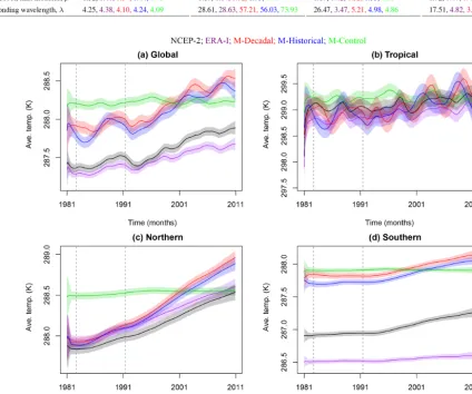
Figure 2 displays the 95 % posterior intervals for baselines η1,t, estimated using the DLM model introduced in Sect. 3.1.
The control run baseline estimates are noticeably flat relative to the baselines inferred for the other types of simulation and for the reanalysis products. This difference is expected – the control run lacks year-to-year changes in external forcings (and therefore the baseline should reflect only random noise, as discussed in Sect. 3.3), whereas the reanalysis products and the historical and decadal prediction runs are affected by time-varying anthropogenic and natural forcings. Within each region, the control baselines are a reference to which we can compare the baselines of the externally forced runs. This comparison (within each region) shows secular temperature increases over the period from 1981 to 2010, consistent with warming of the Earth’s surface in response to time-increasing net anthropogenic forcing.
Note that the surface temperature baseline has a larger overall trend in the historical and decadal prediction runs than in NCEP-2 and ERA-I. This discrepancy in the simu-lated and observed warming rates is at least partly resimu-lated to the omission of the observed early 21st century increase in stratospheric volcanic aerosols in the model historical and decadal prediction simulations (Solomon et al., 2011). In the real world, the cooling caused by this post-2000 increase in stratospheric volcanic aerosols offset part of the anthro-pogenic warming signal (Schmidt et al., 2014).
sur-Table 1.Model baseline discount factorδbasemodand observation baseline discount factorδobsbase. DLM smoothed estimates of level one variance,
V. AR orderqand MAP of AR varianceσ2. Overall maximum modulus with∗indicating correspondence to real roots, maximum complex modulus, and corresponding wavelength (months) calculated from the AR MAP characteristic polynomial.
Figure 2.Baseline temperature estimates which capture long-term externally forced changes (as well as short-term cooling responses to volcanic eruptions). Different line colors denote the type of simulation and the reanalysis product. The top panels represent global(a)and tropical(b)regions; the bottom panels represent the Northern(c)and Southern hemispheres(d). Vertical lines indicate the volcanic eruptions of El Chichón in 1982 and Pinatubo in 1991.
face cooling signals associated with the major eruptions of El Chichón in 1982 and Pinatubo in 1991 (Santer et al., 2001). Because averaging over larger domains damps spa-tial noise, volcanic cooling signals are more pronounced in the global-spatial average, and are more noisy in the smaller-scale tropical averages. The surface cooling signals caused by El Chichón and Pinatubo are markedly smaller in the Northern Hemisphere and Southern Hemisphere averages
regions. The selection of high discount factors suggests that the externally forced longer-term variability in both hemi-spheres was very close to linear. Alternately, the baseline temperatures for the tropical region are estimated with much lower discount factors (see Table 1), indicating the externally forced longer-term variability in the tropics was more vari-able. Any shorter-term forced variability not captured by the baselines will be reflected in the residuals. As a sensitivity study (also mentioned in Sect. 3.3), we considered more flex-ible baselines which incorporated more variability, and there-fore resulted in less variability in the residuals. Although we found the results of the analysis on the residuals robust with respect to the specification of variability of the baseline, further investigation of the differences in the amplitude of the global-average and hemispheric-average volcanic signals may be of interest.
Figure 2 also yields many other features of interest, such as differences in the mean temperature in 1981. Because the decadal prediction runs are initialized from observed ocean temperature and sea ice data, it is not unreasonable to expect that at the time of initialization in 1981, the mean surface temperature in these simulations should be close to the mean temperature of the two reanalysis products. This is the case for the Northern Hemisphere and tropical averages, but not for the averages over the other two regions. The largest mean state differences in 1981 are in the Southern Hemisphere, where the decadal prediction runs are noticeably warmer than either reanalysis. Because this Southern Hemisphere bias is large, it also influences the global temperature average.
One possible interpretation of this large Southern Hemi-sphere bias is that it may arise due to differences between the observed sea surface temperature (SST) data sets used as boundary conditions for the two reanalyses and the sur-face temperature data selected for the initialization of the MIROC5 decadal prediction runs. Observational SST uncer-tainties are likely greater in the more poorly sampled South-ern Hemisphere than in the NorthSouth-ern Hemisphere – which may explain why the 1981 warm bias in the decadal predic-tion runs is largest in the Southern Hemisphere. Addipredic-tion- Addition-ally, the land surface temperature is better sampled in 1981 than the SST. This could also be a cause of bias, as there is a larger contribution from the land surface temperature in the Northern Hemisphere and tropical regions than in the South-ern Hemisphere.
The use of different observational SST data sets may also explain why the two reanalyses show the largest mean state differences in the Southern Hemisphere. An alternative (and not mutually exclusive) interpretation is that the “between reanalysis” mean state differences reflect the sparser obser-vational coverage in the Southern Hemisphere, and a larger Southern Hemisphere imprint of structural differences be-tween the NCEP-2 and ERA-Interim forecast models (e.g., in terms of physics, parameterizations, resolution, and data assimilation systems).
Note that the model versus reanalysis warm biases men-tioned above do not only pertain to the decadal prediction runs – they also affect the historical and control simulations. In all four spatial domains considered, the model-generated baseline temperatures are consistently warmer than in either reanalysis product. Further, the baseline temperatures in the decadal prediction integrations do not appear to exhibit ap-preciable post-initialization secular drift, and are similar to the baseline temperatures in the historical runs. This im-plies that our DLM model is primarily capturing the exter-nally forced component of surface temperature changes in MIROC5, and that the amplitude and structure of this forced response is relatively insensitive to whether the simulation is “free running” or initialized from observations.
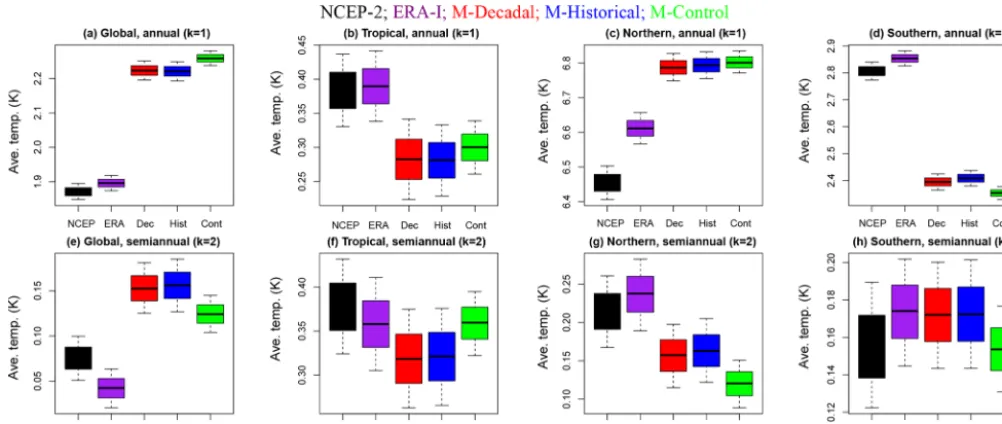
Figure 3 illustrates the 95 % posterior intervals of the sea-sonal amplitudesα1k,t fork=1,2 (i.e., for the amplitudes of the annual and semiannual cycles, respectively). Amplitudes were estimated using the DLM model in Sect. 3.1. For all four spatial domains, the harmonicsk=3 andk=4 (corre-sponding to the trimestral and quarterly cycles, respectively) are very close to zero and indistinguishable from one an-other; therefore, they are not shown. Results for the annual and semiannual cycles are more interesting. Consider the re-analyses first. For all four spatial domains, and for bothk=1 andk=2, NCEP-2 and ERA-I yield very similar amplitudes. The only significant difference between the two reanalyses is in the Northern Hemisphere, where the ERA-I annual cycle amplitude is markedly higher than in NCEP-2.
For all spatial domains except the tropics, and for all three types of simulation, the MIROC5 annual cycle amplitudes differ significantly from those in either reanalysis product. Model versus reanalysis differences in annual cycle ampli-tude are most pronounced in the Southern Hemisphere. The sign of the model annual cycle biases is not consistent across domains. In the tropics and Southern Hemisphere, the annual cycle amplitude is smaller in the simulations than in the re-analyses. In the other two domains, however, the annual cy-cle amplitude is larger in the simulations than in NCEP-2 and ERA-I. We do not find any cases in which there are signifi-cant amplitude differences between the three types of model simulation.
Figure 3.Posterior amplitude samples for harmonicsk=1, 2. Varying model versus reanalysis differences are seen across domains; however, we do not find any cases in which there are significant amplitude differences between the three types of model simulation. Whiskers indicate the maximum and minimum values and boxes indicate the 95 % posterior intervals. Different colors denote the type of simulation and the reanalysis product.
variability acting on a range of different timescales, such as the Madden–Julian Oscillation, ENSO, and the Interdecadal Pacific Oscillation.
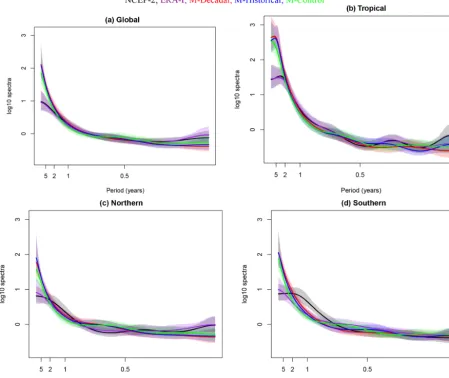
Other features of Fig. 4 are also noteworthy. First, within each region, the spectra for the three different types of MIROC5 simulation are very similar. This suggests that the DLM method applied here has consistently estimated the in-ternally generated component of surface temperature within each region from (1) the significant externally forced com-ponents of temperature changes in the historical runs, and (2) the combined effects of external forcing and any post-initialization drift in the decadal prediction simulations. Sec-ond, at the lowest frequencies, model spectral densities are higher than in NCEP-2 and ERA-I, and the 95 % posterior intervals of nearly all of the simulated spectra do not overlap with the reanalysis spectra. This difference in the amplitude of simulated and observed variability (which is most pro-nounced in the tropics) is consistent with findings obtained elsewhere for multi-model analyses of tropospheric temper-ature (Santer et al., 2018). A model bias in the opposite di-rection to that found here (i.e., a systematic underestimate of the amplitude of observed internal variability on multi-decadal timescales) would be more concerning – such an er-ror would spuriously inflate signal-to-noise ratios for anthro-pogenic signal detection (Santer et al., 2018). We caution, however, that the inference on “observed” estimates of inter-nal variability on multi-decadal timescales is limited by the relatively short (30-year) time-period.
Recall from Sect. 3.4 that the presence of complex roots points towards the existence of quasi-cyclical temperature
variations. The results in the fifth row of Table 1 indicate that complex roots are only consistently obtained for the tropical domain. For all other domains, the characteristic polynomials from the AR models are dominated by real roots. This suggests that the tropics – which are strongly affected by the El Niño–Southern Oscillation – are captur-ing some quasi-periodic temperature variability associated with the occurrence of El Niños and La Niñas. Confirma-tion of this quasi-periodicity comes from the fact that the tropics are also the only domain where the maximum mod-uli of the reciprocal complex roots of the polynomials ex-ceed 0.8 for both reanalyses and for all three types of sim-ulation (see results in the sixth row of Table 1). The wave-lengths for the tropical quasi-periodic variability are approx-imately 28.6 months (2.38 years) for the reanalysis prod-ucts, 57.2 months (4.77 years) for the decadal prediction run, 56 months (4.67 years) for the historical simulation, and 73.9 months (6.16 years) for the control run. The apparent absence of quasi-periodic behavior on longer timescales is probably (at least in part) a reflection of the relatively short record lengths considered here.
sim-Figure 4.MAP AR log10spectra normalized with respect to white noise for each climate simulation by region with the 95 % posterior inter-vals shaded. Instead of the frequencyω, thexaxis is labeled at select years (2π/12ω). Different line colors denote the type of simulation and the reanalysis product. The top panels represent global(a)and tropical(b)regions; the bottom panels represent the Northern Hemisphere(c) and Southern Hemisphere(d).
ulations are further removed from the white-noise reference spectrum. The systematically lower TVD values for NCEP-2 and ERA-I may partly reflect the fact that both reanalyses ex-hibited decadal temperature variability that was consistently smaller than in the MIROC5 simulations. The largest TVD values for the reanalyses and the model simulations are in the tropics, indicating that tropical temperature variability is most clearly distinguishable from white noise. This is con-sistent with the abovementioned finding that the discrepancy between low-frequency temperature variability in the reanal-yses and the MIROC5 simulations is largest in the tropics.
Figure 5e–h display results for the comparison between the model spectra and the NCEP spectrum. The range of TVD values for the NCEP spectrum versus itself is simply a reflec-tion of posterior sampling variability. The global and tropi-cal regions show distinct differences between the reanalysis
products and the three sets of simulations, with little or no overlap between the 95th percentiles of the reanalyses and the 5th percentiles of the simulations. The tropical region exhibits the most significant difference between the NCEP spectrum and the simulated spectra; this is likely due to the abovementioned discrepancies in low-frequency variance. It may also reflect the fact that the identified quasi-periodic component of tropical temperature variability had a longer timescale in the three sets of simulations than in the reanaly-sis products.
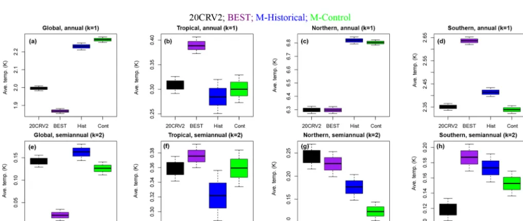
5 Result from the 63-year assessment of large-scale
temperature
Jan-Figure 5.(a–d)TVD calculated fromφsamples with white noise as the reference.(e–h)TVD calculated fromφsamples with the MAP NCEP spectrum as the reference. Larger TVD values indicate higher discrepancy between spectral densities. Whiskers indicate the maximum and minimum values and boxes indicate the 95 % posterior intervals. The scenario or observational product is indicated using colors. From left to right: global(a, e), tropical(b, f), Northern Hemisphere(c, g), and Southern Hemisphere(d, h).
uary 1950 to December 2012. Excluding the decadal experi-ment which does not include realizations covering more than 30 years, we use MIROC5 simulation data from the histori-cal and control experiments. We compare the model results to the results obtained from the 20CRV2 and BEST obser-vational products. Again, we would like to reiterate that the results are not meant to be directly compared between each region. Table 2 provides summaries of the DLM and AR es-timated model parameters and posterior inferences for each spatial domain. This includes the baseline discount factors δbasemod andδbaseobs, MAP DLM level one equation varianceV, AR model order q, MAP AR varianceσ2, maximum mod-uli of all reciprocal roots from the AR characteristic poly-nomial based on the posterior means of the AR coefficients, maximum moduli of the reciprocal complex roots, and cor-responding wavelengths (months).
Figure 6 displays the 95 % probability intervals for the DLM estimated baselinesη1,t. The control baseline is seen
to be flatter than the historical baseline, as the control runs do not incorporate changes in the external forcings. However, the historical runs and observational products are affected by changes in anthropogenic forcing, resulting in the tempera-ture increases seen over the period from 1950 to 2012. Cool-ing effects of volcanic eruptions are also evident in the base-lines with lower discount factors (global, tropical, and South-ern Hemisphere), similarly to what is observed in the short-term analysis. In this longer analysis, the Southern Hemi-sphere exhibited more variability, resulting in a lower base-line discount factor (see Table 2) than in the short-term anal-ysis, which has an optimal value close to one (see Table 1).
It is not unexpected for a larger time-span to reflect more temperature variability than a more narrow time-span. The variability in the Northern Hemisphere remains less dynamic than that of the other regions, as is the case for the short-term analysis. This is reflected in a baseline discount factor that is close to one (see Table 2). Again, we see the most variability in the smaller-spatial-scale tropical averages.
Figure 6 also illustrates a distinct discrepancy between the two observational products. This is most noticeable in the global region and the Northern and Southern hemispheres, where 20CRV2 is consistently warmer than BEST. The dis-crepancy is present, but not very strong in the tropics, where BEST is warmer than 20CRV2. It can also be seen that the baseline for the historical simulations is cooler than that of the observational products in the Northern Hemisphere, and warmer than the observational products in the Southern Hemisphere, whereas for the other two regions there are no relevant discrepancies.
Figure 6.Same as in Fig. 2 but for the long-term analysis.
Table 2.Model baseline discount factorδmodbaseand observation baseline discount factorδobsbase. DLM smoothed estimates of residual variance,
V. AR orderqand MAP of AR varianceσ2. Overall maximum modulus with∗indicating correspondence to real roots, maximum complex modulus, and corresponding wavelength (months) calculated from the AR MAP characteristic polynomial.
Figure 8.Same as in Fig. 4 but for the long-term analysis.
distinctly higher. In the Northern Hemisphere the two obser-vational products are indistinguishable. In general, the model versus observation differences in amplitude are less clear, al-though pronounced differences are seen in the annual cycle of the globe and Northern Hemisphere.
observa-tional spectra are indistinguishable within all spatial regions. Furthermore, the model run spectra are also indistinguishable within all spatial regions and exhibit notably higher power in the low frequencies than the observational spectra. This is consistent with the previous 30-year analysis. However, the model versus observational differences seen here are stronger than in the 30-year analysis.
We explore possible quasi-cyclical temperature variations by considering the complex roots of the AR characteris-tic polynomial. Table 2 again indicates that complex roots with moduli exceeding 0.8 are only obtained for the trop-ical domain – most likely reflecting temperature variabil-ity associated with the occurrence of El Niños and La Niñas. The wavelengths for the tropical quasi-periodic vari-ability are approximately 23.27 months (1.94 years) for 20CRV2, 26.18 months (2.18 years) for BEST, 57.12 months (4.76 years) for the historical simulation, and 62.8 months (5.23 years) for the control run. Notice that even in a 63-year record there is an absence of quasi-periodic behavior on long timescales, as was the case for the analysis of the 30-year record. To avoid redundancy, we have omitted the TVD summaries, as they share many similarities with the 30-year analysis.
6 Conclusions
We developed a model diagnostic statistical methodology and protocol that can be generally applied to the assess-ment and comparison of simulations from CMIP models. The methods presented here have two main advantages: the pro-tocol developed is a consistent and statistically principled ap-proach to jointly estimate the components of the temperature time series, and the results incorporate probabilistic uncer-tainty as the approach is model-based. Within this protocol, we applied univariate and multivariate dynamic linear mod-eling (DLM) techniques to estimate two externally forced components of surface temperature time series. These com-ponents contain (1) seasonal information, which is invari-ant from year-to-year, and (2) the time-varying nonlinear re-sponse to combined external forcing by human factors (such as greenhouse gases and particulate pollution) and natural in-fluences (changes in solar irradiance and volcanic activity). The three sets of numerical experiments considered were ini-tialized decadal predictions (not included in the long-term analysis), control runs, and uninitialized simulations of his-torical climate change. Removal of the seasonal and baseline components from the raw temperature data yielded residu-als that primarily provided information on unforced natu-ral internal climate variability. We characterized this inter-nal variability by fitting univariate and multivariate autore-gressive (AR) models to the residuals. As estimates of exter-nally forced climate signals and internal variability depend on the particular domain of interest, we explored the efficacy of our DLM and AR signal and noise identification methods
for four different spatial domains, ranging in scale from the entire globe to the tropics.
We illustrated our approach in both a short-term and long-term analysis using one selected climate model (MIROC5). In the short-term 30-year analysis, estimation of the various temperature components was performed for two reanalysis data sets and for three different types of experiments. Sim-ilarly, in a long-term 63-year analysis, estimation of these components was performed for a 20th century reanalysis, gridded in situ data, and two of the three different simulated experiments. We found significant differences between the observational product data and the model-generated simula-tions in all three temperature components (seasonal, baseline, and internal variability), for both the short- and long-term analyses.
From a climate perspective, two results of our analyses were particularly intriguing. First, we note that the three sets of simulations analyzed here are very different. While temperature variability in the control run arises from inter-nal variability alone, variability in the historical and decadal prediction runs is a mixture of internal variability and re-sponse to external forcing. Additionally, the decadal predic-tion runs may also be influenced by post-initializapredic-tion “drift” in the model climate. Despite these differences in the mix of underlying factors contributing to variability, the simu-lation runs yielded very similar spectral estimates of inter-nal temperature variability within each region – as might be expected given that the same physical climate model is be-ing used for each of the three sets of simulations. This sim-ilarity of the model spectra is reassuring, and implies that our statistical analysis methods are consistently extracting comparable components of internal variability for the sim-ulation data within each region. The second intriguing re-sult emerged from the comparison of the model and ob-servational product temperature variability on multi-decadal timescales. These timescales are important components of the background “noise” against which a gradually evolving anthropogenic warming signal must be detected. If models systematically underestimated natural internal variability on multi-decadal timescales, it would imply that previously ob-tained anthropogenic signal detection results were spuriously inflated by low model noise levels. Consistent with related work involving tropospheric temperature (Santer et al., 2013, 2018), we find no evidence that the MIROC5 model system-atically underestimates the amplitude of low-frequency inter-nal variability inferred from observatiointer-nal product data. Our methodology and results present a novel approach for obtain-ing data-driven estimates of the amplitude of observed multi-decadal temperature variability, thereby providing a more solid observational “target” for model evaluation purposes.
access: 13 August 2018), https://www.esrl.noaa.gov/psd/ (last access: 13 August 2018), and https://www.ecmwf.int/en/forecasts/ datasets/reanalysis-datasets/era-interim (last access: 13 August 2018), respectively. For the long-term analysis, observational record data from the BEST and 20CRV2 are available from http://berkeleyearth.org/data/ (last access: 13 August 2018) and https://www.esrl.noaa.gov/psd/data/gridded/data.20thC_ReanV2. monolevel.mm.html (last access: 13 August 2018), respec-tively. The R package for DLMs, “dlm”, is available online (https://cran.r-project.org/web/packages/dlm/index.html, last access: 13 August 2018).
Competing interests. The authors declare that they have no con-flict of interest.
Acknowledgements. The authors wish to thank Ben Santer, Ana Kupresanin, and Francisco Beltran at LLNL for helpful con-versation. We also thank the editor, associate editor, and referees for their comments. Bruno Sansó was partially funded by the National Science Foundation (grant no. DMS-1513076). Raquel Prado was partially funded by the National Science Foundation (grant no. SES-1461497).
Review statement. This paper was edited by Chris Forest and re-viewed by three anonymous referees.
References
Alvarez, E., C., P., Euan, C., and Ortega, J.: Time se-ries clustering using the total variation distance with ap-plications in oceanography, Environmetrics, 27, 355–369, https://doi.org/10.1002/env.2398, 2016.
Berrisford, P., Kållberg, P., Kobayashi, S., Dee, D., Uppala, S., Sim-mons, A., Poli, P., and Sato, H.: Atmospheric conservation prop-erties in ERA-Interim, Q. J. Roy. Meteor. Soc., 137, 1381–1399, 2011.
Compo, G. P., Whitaker, J. S., Sardeshmukh, P. D., Matsui, N., Al-lan, R. J., Yin, X., Gleason, B. E., Vose, R. S., Rutledge, G., Bessemoulin, P., Brönnimann, S., Brunet, M., Crouthamel, R. I., Grant, A. N., Groisman, P. Y., Jones, P. D., Kruk, M. C., Kruger, A. C., Marshall, G. J., Maugeri, M., Mok, H. Y., Nordli, Ø., Ross, T. F., Trigo, R. M., Wang, X. L., Woodruff, S. D., and Worley, S. J.: The twentieth century reanalysis project, Q. J. Roy. Meteor. Soc., 137, 1–28, 2011.
Dee, D. P., Uppala, S., Simmons, A., Berrisford, P., Poli, P., Kobayashi, S., Andrae, U., Balmaseda, M., Balsamo, G., Bauer, P., Bechtold, P., Beljaars, A. C. M., van de Berg, L., Bidlot, J., Bormann, N., Delsol, C., Dragani, R., Fuentes, M., Geer, A. J., Haimberger, L., Healy, S. B., Hersbach, H., Hólm, E. V., Isak-sen, L., Kållberg, P., Köhler, M., Matricardi, M., McNally, A. P., Monge-Sanz, B. M., Morcrette, J.-J., Park, B.-K., Peubey, C., de Rosnay, P., Tavolato, C., Thépaut, J.-N., and Vitart, F.: The ERA-Interim reanalysis: Configuration and performance of the data assimilation system, Q. J. Roy. Meteor. Soc., 137, 553–597, 2011.
Derpanis, K. G.: The bhattacharyya measure, Mendeley Computer, 1, 1990–1992, 2008.
Euan, C., Ombao, H., and Ortega, J.: Spectral syn-chronicity in brain signals, Stat. Med., 37, 2855–2873, https://doi.org/10.1002/sim.7695, 2018.
Fujiwara, M., Wright, J. S., Manney, G. L., Gray, L. J., Anstey, J., Birner, T., Davis, S., Gerber, E. P., Harvey, V. L., Hegglin, M. I., Homeyer, C. R., Knox, J. A., Krüger, K., Lambert, A., Long, C. S., Martineau, P., Molod, A., Monge-Sanz, B. M., San-tee, M. L., Tegtmeier, S., Chabrillat, S., Tan, D. G. H., Jack-son, D. R., Polavarapu, S., Compo, G. P., Dragani, R., Ebisuzaki, W., Harada, Y., Kobayashi, C., McCarty, W., Onogi, K., Paw-son, S., Simmons, A., Wargan, K., Whitaker, J. S., and Zou, C.-Z.: Introduction to the SPARC Reanalysis Intercomparison Project (S-RIP) and overview of the reanalysis systems, At-mos. Chem. Phys., 17, 1417–1452, https://doi.org/10.5194/acp-17-1417-2017, 2017.
Gelman, A., Stern, H. S., Carlin, J. B., Dunson, D. B., Vehtari, A., and Rubin, D. B.: Bayesian data analysis, Chapman and Hall/CRC, New York, USA, 2013.
Gibson, P. B., Perkins-Kirkpatrick, S. E., Alexander, L. V., and Fis-cher, E. M.: Comparing Australian heat waves in the CMIP5 models through cluster analysis, J. Geophys. Res.-Atmos., 122, 3266–3281, 2017.
Imbers, J., Lopez, A., Huntingford, C., and Allen, M.: Sensitivity of climate change detection and attribution to the characterization of internal climate variability, J. Climate, 27, 3477–3491, 2014. Kalnay, E., Kanamitsu, M., Kistler, R., Collins, W., Deaven, D.,
Gandin, L., Iredell, M., Saha, S., White, G., Woollen, J., Zhu, Y., Chelliah, M., Ebisuzaki, W., Higgins, W., Janowiak, J., Mo, K. C., Ropelewski, C., Wang, J., Leetmaa, A., Reynolds, R., Jenne, R., and Joseph, D.: The NCEP/NCAR 40-year reanalysis project, B. Am. Meteorol. Soc., 77, 437–471, 1996.
Kanamitsu, M., Ebisuzaki, W., Woollen, J., Yang, S.-K., Hnilo, J., Fiorino, M., and Potter, G.: Ncep–doe amip-ii reanalysis (r-2), B. Am. Meteorol. Soc., 83, 1631–1643, 2002.
Kay, J., Deser, C., Phillips, A., Mai, A., Hannay, C., Strand, G., Ar-blaster, J., Bates, S., Danabasoglu, G., Edwards, J., and Holland, M.: The Community Earth System Model (CESM) large ensem-ble project: A community resource for studying climate change in the presence of internal climate variability, B. Am. Meteorol. Soc., 96, 1333–1349, 2015.
Kirtman, B., Power, S., Adedoyin, A., Boer, G., Bojariu, R., Camil-loni, I., Doblas-Reyes, F., Fiore, A., Kimoto, M., Meehl, G., Prather, M., Sarr, A., Schar, C., Sutton, R., Oldenborgh, G., Vec-chi, G., and Wang, H.: Near-term climate change: projections and predictability, in: Climate Change 2013: The Physical Science Basis. Contribution of Working Group I to the Fifth Assessment Report of the Intergovernmental Panel on Climate Change, Cam-bridge, UK and New York, USA, 2013.
Kopp, G. and Lean, J. L.: A new, lower value of total solar irra-diance: Evidence and climate significance, Geophys. Res. Lett., 38, L01706, https://doi.org/10.1029/2010GL045777, 2011. Meehl, G. A., Goddard, L., Murphy, J., Stouffer, R. J., Boer, G.,