Enhancement of ECG using Empirical Mode Decomposition

Available online:

https://edupediapublications.org/journals/index.php/IJR/

Enhancement of ECG using Empirical Mode

Decomposition

B.SHOBA RANI

ASSOCIATE PROFESSOR DEPT OF ECE CHAITANYA INSTITUTE

OF TECHNOLOGY & SCIENCE

Abstract: This paper presents a new method based on empirical mode decomposition for enhancement of ECG (Electrocardiogram) signals. ECG signal has been widely used for diagnosis purposes of heart diseases. So a good quality ECG free from artifacts is required by physicians to easily and accurately diagnosis the physiological and pathological phenomena. However ECG recordings are often corrupted by artifacts that does not allow accurate diagnosis of heart conditions. So these artifacts need to be eliminated from the ECG for better clinical evaluation. Two dominant artifacts present in ECG recordings are Power line interference and Baseline Wander. In this paper we used empirical mode decomposition for denoising of Power line interference and Baseline Wander. We have used MIT- BIH arrhythmia and Fantasia database to validate the efficiency of method. Simulations were carried out in MATLAB environment. The results shows that this method is able to remove both Power line interference and Baseline Wander with minimum distortion just in a single step.

Keywords: Electrocardiogram (ECG), Empirical Mode Decomposition (EMD), ECG enhancement, Denoising , Power line interference , Baseline Wander.

1. Introduction

The electrocardiogram (ECG) is the recording of cardiac activity and is extensively used for diagnosis of heart diseases[1]. A typical ECG tracing of normal heartbeat consists of a P wave , QRS complex , and a T wave. Figure 1 shows the normal ECG trace. Transmission of ECG often introduces noise due to poor channel conditions and thus corruption of signal. Noise needs to be attenuated in order to obtain a clean ECG signal for accurate diagnosis of heart condition. Different types of noises that may corrupt ECG are [3].

1. Power Line Interference. 2. Baseline Wander. 3. Electrode Contact Noise. 4. Muscle Contraction. 5. Motion Artifacts.

Among these noises the most common are Power Line Interference and Baseline Wander. Power line interference consists of 50 or 60Hz pickup and harmonics, which can be modelled as sinusoids and combination of sinusoids. It is due to electromagnetic interference from electric power systems and also may be due to loose contacts contacts on the patient’s cable as well as dirty electrodes. The most common cause of 50 or 60 Hz interference is disconnected electrode resulting in a very strong disturbing signal, and therefore needs quick action. Baseline Wander[4] is variation in isoelectric line of ECG. It is a low frequency artifact that occurs in a chest-lead ECG signals. Baseline wander is usually caused by respiration or movement of subject due to breathing or coughing. Effect of temperature and bias variations on the instruments and amplifiers can also cause drift in ECG baseline voltage.

The process of extracting the required components while rejecting the background noise is called enhancement of ECG signal. The goal of ECG signal enhancement is to separate the valid signal components from the undesired artifacts, so as to present an ECG that facilitates easy and accurate visual interpretation. So in this paper we enhance the ECG signal by reduction of power line interference and Baseline Wander Removal so that proper diagnosis of heart diseases can be done.

Figure 1 : Normal ECG [2]

Many techniques were introduced for ECG signal enhan- cement such as wavelet transforms[5-7], filter banks[8], adaptive filtering[9], singular value decomposition[10], Independent component analysis[11]. Among these wavelet based method is very suitable tool for denoising of Gaussian type noise in various areas.

P a g e | 2770 ���

���

stationary signals. It also serves as an alternative to methods such as wavelet analysis, the Wigner-Ville distribution, and the short-time fourier transform.

2.

Empirical Mode Decomposition

f. If not, use h1(t) as the new data and repeat steps 1 to 6 until ending up with an IMF.

Some stopping criteria are used to terminate the sifting process. A commonly used criterion is the sum of difference (SD) and given by

Empirical Mode Decomposition method was first presented

by Haung et al. [12]. The empirical mode decomposition SD=∑� |ℎ���(t)- ℎ� (t)| ² ⁄ℎ² ���(t ) (1) (EMD) algorithm has been designed for the time-frequency

analysis of real-world signals. EMD is an adaptive decomposition with which any complicated signal can be decomposed into finite and often small number of its intrinsic mode functions (IMF) which represent zero-mean amplitude and frequency modulated components, so that the application of Hilbert transform to these intrinsic mode functions provides meaningful instantaneous frequency estimates. Other data analysis methods, like Fourier and wavelet-based methods, require some predefined basis functions to represent a signal. The EMD represents a fully data-driven, unsupervised signal decomposition and does not need any a priori defined basis system and thus making EMD suitable for the analysis of nonlinear and nonstationary signals. EMD also satisfies the perfect reconstruction property, i.e. superimposing all extracted IMFs together with the residual slow trend reconstructs the original signal without information loss or distortion.

The aim of the EMD is to decompose the signal into a sum of intrinsic mode functions (IMFs). An IMF is defined as a function that satisfies the following requirements:

(a)In a whole data set, the number of extrema and number of zero crossings must be either equal or differ at most by one.

(b)At any point, the mean value of envelope defined by local maxima and envelope defined by local minima is zero.

2.1. Sifting Process

Some of the assumptions made for decomposition are: [13]

 The signal has at least two extrema: one maximum and one minimum

 The characteristic time scale is defined by the time lapse between the extrema.

 If the signal has no extrema but has inflection points, then the signal can be differentiated one or more times to find the extrema.

The idea of finding the IMFs relies on subtracting the highest oscillating components from the data by a step by step process which is called sifting process. A systematic way to extract the IMFs is called the Sifting Process and is described below.

a. Identify all the extrema (both maxima and minima) of x(t).

b. Generate the upper and lower envelopes ( u(t) and l(t) ) by connecting the maxima and minima points by cubic spline interpolation.

c. Compute the mean as: m1(t)= ( u(t) + l(t))/2

d. Since IMF should have zero local mean ; subtract out m1(t) from the x(t) to get h1(t) :h1(t) = x(t)-m1(t) . e. Check whether h1(t) is an IMF or not.

When the SD is smaller than a threshold, the first IMF ��(�) is obtained and it is denoted as �_�(�) =h1(t). To get the remaining IMFs, ��(�) is subtracted from original data to get the residual signal ��(t ).

��(t )=x(t)− ��(�) (2)

The residual now contains the information about the components of longer periods. The process to obtain more IMFs can be stopped when the component ��(t ) becomes less than a predetermined value or becomes a monotonic function , or constant ,or a function with only one maxima and one minima from which no more IMFs can be extracted. The subsequent IMFs and residues are compared as

��(t )− ��(�) = ��(t )

⋮

����(t )− ��(�) = ��(t ) (3)

At the end of decomposition , the original signal x(t) will be represented as sum of IMFs plus a residue Signal

X(t)=∑� ��(t)+ ��(t ) (4)

where the �� (�) are the n-empirical modes and the component ��(t ) is the mean trend or a constant.

3.

Methods and Results

For experimental study we have used the MIT/BIH arrhythmia database and Fantasia database from physionet [14]. Simulations were carried out in MATLAB environment.

Reduction of Power Line Interference

The basic principle of enhancement of ECG signal using EMD is expressing the noisy ECG as sum of a series of IMFs. The 1st IMF contains nothing but high frequency noise. Next few IMFs contains both noise and information and the last IMFs usually contain low frequency. Power line interference is a high frequency noise. So we can easily eliminate this component.

Available online:

https://edupediapublications.org/journals/index.php/IJR/

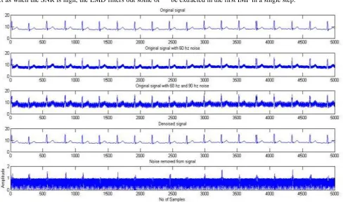
which we can remove the power line noise just in a single step as compared to [15] ,a three step process and [16] a four step process. In this we use approach that when SNR is fairly low, the 60 Hz noise is removed in the first IMF but when SNR is high a pseudo noise is added at a higher frequency to

filter out the 60 Hz noise. The pseudo noise helps to filter out the important lower–frequency signal components along with the power line noise leaving the other

signal frequencies

the power line noise. So by applying this technique noise can

intact as when the SNR is high, the EMD filters out some of be extracted in the first IMF in a single step.

Figure 2. Reduction of Power Line Interference

Removal of noise from ECG signal was accomplished by the following algorithm.

a. The first step is to add a pseudo 90-Hz sinusoidal noise to the ECG corrupted with low-level 60-Hz noise.

b. Second step is to perform EMD algorithm on noisy signal which extracts the 60-Hz noise in first IMF.

c. In the next step, subtract the resulting first IMF

original signal (let x(t)) . Then we add 60 Hz noise to the original signal (i.e. x1(t)=x(t)+60 Hz sinusoidal component) which is shown in second plot. Now if the SNR is low then by applying EMD it remove 60 Hz noise just by subtracting the first IMF from the x1(t). But if SNR is high then we add 90 Hz noise to x1(t) (i.e. x2(t)=x1(t)+ 90 Hz noise), therefore can remove 60 Hz noise just by subtracting the first IMF from x2(t).

component from the noisy ECG to waveform.

obtain the filtered

Figure 3 shows the Power spectral density (PSD) plot of original signal with 60 Hz noise in the first plot and with For experimental study we have used MIT/BIH arrhythmia

Available online:

https://edupediapublications.org/journals/index.php/IJR/

(3) denoised signal.

Figure 4. Baseline Wander Removal. First part shows original signal with its PSD plot and second part shows signal after Baseline Wander Removal.

Baseline wander Removal

Baseline wander (BW) is a low-frequency artifact in ECG recording which is mainly generated by the patient motions,

of baseline from the ECG signal has been proposed by [1] in which partial reconstruction of the ECG signal from the IMF obtained by the decomposition of the input ECG signal is used. This is done in a way to remove low frequency

respires and others. The body movement due to coughing or

breathing is the major cause of the BW.

P a g e | 2773

Many techniques have been used for Baseline Wander removal. Most are based on digital filtering, wavelet

As the Baseline Wander is usually a low frequency phenomenon , it is involved mainly in the last several approach [18]. Others are discussed in[19]. In this paper we

used a new approach for removing Baseline wander from ECG signal using Empirical Mode Decomposition. In this first we decompose the signal into sum of intrinsic mode functions (IMFs) using EMD. The use of EMD for removal components of IMFs. Depending on the properties of the IMFs we subtract directly the sum of higher order IMFs from ECG to achieve the correction of BW in ECG. In this paper we subtract the sum of the last three or four IMFs , which

can be regarded as Baseline Wander, from the ECG signal [20].

For the experimental study we have used the FANTASIA database f1y06 which is corrupted by Baseline Wander. Figure 4 shows the Baseline Wander Removal. First plot shows the original signal with Baseline Wander. Second plot shows the PSD of original signal which shows that signal contains the low frequency components,so the baseline wander. So we removed the baseline wander by applying EMD to decompose the signal into IMFs and thus subtract the higher order IMFs from the original signal which usually contains the low frequency components. Third plot shows the signal after removal of baseline wander and the last shows that low frequency components are removed from the signal which causes the Baseline Wander.

We can also remove both high frequency noise and Baseline wander simultaneously by subtracting the First IMF and last few IMFs (usually three or four IMFs) depending on the signal.

4.

Conclusions

In this paper Enhancement of ECG is done by removing both the power line interference and Baseline Wander by using a method Empirical Mode Decomposition. The results shows that EMD method is able to remove both the power line interference and Baseline Wander from the ECG just in a single step compared to other techniques. Therefore it is takes less computational time and hence best suited for clinical purposes for analysis of ECG signal.

5.

Acknowledgements

Foremost, I would like to express my sincere gratitude to Mr. Vikramjit Singh for his valuable guidance and full support in carrying out this work. At last but not the least my gratitude towards my parents and friends, I would also like to thank God for the strength that keep me standing and for the hope that keep me believing that this report would be possible.

References

[1] Manuel Blanco-Velasco, Binwei Weng & Kenneth E. Barner, “ECG signal denoising and baseline-wander correction based on the empirical mode decomposition” ,Computers in Biology and Medicine 38, pp. 1-13, 2007. [2] http://en.wikipedia.org/wiki/File:SinusRhythmLabels.sv g [3] Ms. Geeta Kadam & Prof.P.C.Bhaskar ,“ Reduction of

power line interference in ECG signal using FIR filter”, IJCER ,Vol. 2 , pp. 314-319, 2012.

[4] Binwei Weng , Manuel Blanco-Velasco & Kenneth E. Barner, “Baseline Wander Correction in ECG by Empirical Mode Decomposition”, proc. IEEE 32nd Annual Northeast Bioengineering conference ,pp.135- 136, 2006.

[5] P.E. Tikkanen ,“Nonlinear wavelet and wavelet packet denoising of electrocardiogram signal”, Biol. Cybern. 80 (4), pp. 259–267, 1999.

[6] C.Y.-F. Ho, B.W.-K. Ling , & T.P.-L. Wong, “ Fuzzy multiwavelet denoising on ECG signal”, Electron. Lett. 39 (16), pp. 1163–1164, 2003.

[7] E. Ercelebi, “Electrocardiogram signals de-noising using lifting-based discrete wavelet transform”, Comput. Biol. Med. 34 (6), pp. 479–493, 2004.

[8] V.X. Afonso, W.J. Tompkins, T.Q. Nguyen, K. Michler & S. Luo, “ Comparing stress ECG enhancement algorithms” , IEEE Eng. Med. Biol. Mag. 15 (3) , pp. 37–44, 1996.

[9] V. Almenar, A. Albiol, “ A new adaptive scheme for ECG enhancement”, Signal Process. 75 (3), pp. 253- 263., 1999.

[10]J.S. Paul, M.R.S. Reddy & J. Kumar, “Data processing of stress ECG using discrete cosine transform” , Comput. Biol. Med. 28 (6), pp. 639–658, 1998.

[11]A.K. Barros, A. Mansour & N. Ohnishi,“Removing artifacts from electrocardiographic signals using independent components analysis”, Neurocomputing 22, pp. 173–186, 1998.

[12]N. E. Huang, Z. Shen, S. R. Long, M. L. Wu, H. H. Shih, Q. Zheng, N. C. Yen, C. C. Tung & H. H. Liu, “The Empirical Mode Decomposition and Hilbert spectrum for nonlinear and non-stationary time series analysis” , Proc. Roy. Soc. London A, Vol. 454, pp. 903–995, 1998.

[13]Harishwaran Hariharan, “Image Fusion and Enhancement via Empirical Mode Decomposition” , Journal of Pattern Recognition Research ,vol.1 , pp. 16- 31, 2006.

[14]http://www.physionet.org/physiobank/database/mitdb : The MIT-BIH Arrhythmia Database.

[15]Z. Zhao & Y. Chen, “A new method for removal of baseline wander and power line interference in ECG signals” , Proceedings of the Fifth International Conference on Machine Learning and Cybernetics, pp.4342, 2006.

[16]Binwei Weng, Manuel Blanco-Velasco, & Kenneth E. Barner , “ECG Denoising Based on the Empirical Mode Decomposition,” Proc. 28th IEEE EMBS Annual International Conf. , pp.1-4 , 2006.

[17]Amit J. Nimunkar & Willis J. Tompkins,“EMD-based 60-Hz noise filtering of the ECG,” proc. 29th IEEE EMBS Annual International Conf. , pp.1904-1907, 2007.

P a g e | 2774

Trends in Technology, 2011.

[19]Rahul Dev,“Different Techniques to Remove Baseline Wander from ECG Signal : A Review”, proc. VSRD- IJEECE, Vol. 2 (7), pp.532-537,2012.

[20]Na pan, Vai Mang I, Mai Peng Un & Pun Sio Hang , “Accurate Removal of Baseline Wander in ECG Using Empirical Mode Decomposition” , proc IEEE international conf. , pp.177-180, 2007.

AUTHOR DETAILS