ANALYSIS OF QUANTITATIVE GENE ACTION BY CONSTANT PARENT REGRESSION AND RELATED TECHNIQUES

ANALYSIS OF QUANTITATIVE GENE ACTION BY CONSTANT P A RE NT REGRESSION AND RELATED TECHNIQUES’

BRUCE GRIFFING Iowa State College, Ames, Iowa

Received November 14, 1949

NALYSIS of multigenic or quantitative inheritance is one of the im-

A

portant problems of theoretical and applied genetics. Such analysis re- quires techniques of a different nature from those used in studying individual genes of large effect. The techniques thus far devised have not been wholly satisfactory, and for this reason new methods of analyzing quantitative in- heritance are of considerable interest. A relatively new method, the constant parent regression technique, is reviewed and extended in this paper.

There is a considerable body of evidence to demonstrate that typical quan- titative characters are controlled by a large number of gene pairs. It is assumed that the following statements are corollaries of this multigenic nature of in- heritance: (1) linkage results because the large number of quantitative genes for a particular trait are located on a relatively small number of chromosome pairs, and (2) in general, the effect of each gene pair is relatively small. Be- cause of this low order of effect of individual genes, it is necessary to study the action of these genes “en masse” by statistical techniques. This obviously results in inferences about the average properties of a set of quantitative genes. T o estimate the average gene action one may construct models involving different types of gene interaction and choose the model which best fits the experimental data. I n thus reducing the total gene action entering into the expression of a complex characteristic to that of a simple model, it cannot be assumed that all genes behave in the manner prescribed by the chosen model. I n fact, it has been suggested that quantitative genes probably have as diverse types of action as the so-called qualitative ones and differ from qualitative genes only in magnitude of effect. However, it has been shown in various quantitative traits that the system of genes involved does have average properties which are measurable. Estimation of these group genetic parameters is the objective of a statistical analysis, and these estimated parameters are associated with a gene model. The principal approach that has developed over the years involves, (1) a description of frequency distributions resulting from segregating populations by use of first, second, and third moments, and

( 2 ) a partitioning of variances into components. Most of the techniques have been summarized by MATHER (1949).

Use of segregating populations offers certain advantages but entails both theoretical and practical difficulties. First, with segregation, linkage effects are generated which contribute to the genotypic variance. This complex prob- lem has been dealt with to some extent by MATEER (1949). Second, a large

Journal Paper No. J-1719 of the IOWA AGRICULTURAL EXPERIMENT STATION, Ames, Iowa. Project No. 250.

304 BRUCE GRIFFING

number of individuals are needed to estimate properly the parameters of any one particular genetically segregating population. For example: justi- fiably to partition the variance of an Fz, the experimenter needs to include a fairly large number of F3 or biparental families each with adequate number of individuals to estimate their own distributions. This leads t o the physical dif- ficulty of making observations on a vast number of individuals. If the char- acteristics involved are functions of indeterminate type of growth, such as yield of tomatoes, the amount of work becomes tremendous. Third, difficulties arise in designing experiments from which estimates of different populations are accurate and comparable. There is also the problem of confounding genetic and block effects in a replicated experiment.

By considering only the non-segregating generations (homozygous parents and Fls) the constant parent regression method, evolved by Hull (1946, 1947), considerably reduces the previously mentioned sources of error. Since the PIS and Fls are not segregating, relatively few plants are needed to estimate the expected genotypic values. The actual number necessary depends on the heritability of the traits involved, and the accuracy may be increased to any practical desired level by merely increasing the number of plants. Variance within a line is assumed to be entirely environmental and thus, with appropri- ate sampling techniques, an analysis of the source of these environmental variations is provided. Experimental designing presents no problems and there is no genetic confounding. (There is, of course, a genotypic-environmental in- teraction which may be estimated.)

Linkage disturbs the constant parent regression analysis only in the sam- pling procedure of obtaining the set of parents used from all theoretical possi- ble homozygous genotypes. I n populations resulting from recent hybrid origin, linkages existing in the original parental types may reduce the probability of occurrence of some gene combinations and raise the probability of obtaining others. It can be demonstrated that coupling linkages do not affect the con- stant parent regression results whereas repulsion linkages may give rise to some pseudo-overdominance as measured by the second order regression co- efficient. However, with random mating over a period of time the coupling and repulsion phases are expected to become equally frequent in the popula- tion, and thus, the effect of linkage in sampling parental lines disappears. The possibility of linkage effect should not be overlooked but in most cases is probably of little concern.

Experiments with segregating populations generally involve only two orig- inal parents. On the other hand, the PI-FI test is conducted with a variety of different parents, thus providing a wider sampling of the available germ- plasm, and allowing broader inferences to be made from the result obtained. By using a number of parents, the experimenter interested in more than one characteristic should be able to choose lines which collectively give desired ranges of expression in all traits. This might be difficult to do when only two parents must be chosen.

QUANTITATIVE GENE ACTION 305 bility and of phenotypic and genotypic correlations. These estimates may be used to develop discriminant function selection indices if desired (see GRIFFING

1948).

The main disadvantages of the P1-Fl technique are that estimation of gene number or number of effective factors (MATHER 1949), detection of major genes and examination of gene-chromosome relationships which could involve linkage and phase of linkage are not directly possible.

CONSTANT PARENT REGRESSION METHOD

The following presentation will consider the experimental situation in which a set of inbred (homozygous) lines are available together with all possible

F1 combinations of these lines. These restrictions are not entirely necessary in that not all Fls need be present, different males and females may be used, and F2s and later generations may be considered (HULL 1947a). However, for simplicity the above mentioned restrictions will be imposed. Generally, one set of Fls is used and not the reciprocals, i.e. Fij = Fji in table 1.

Notation is as follows:

Pi = ith parent

Fij = F1 (or hybrid) of ith and j t h parents c.p. = constant parent (homozygous)

F..=F.. _{11 11}

c.p.r. = constant parent regression, also noted as bp.

F1 and Fij are used interchangeably. The term “F1” is used in the general sense, and Fij is used more specifically to indicate the F1 of the

ith

and jth

parents.

(1) “n” parents are crossed in all possible combinations of pairs to give

TABLE 1

Combination of n inbred lines to give all possible Fl’s.

pa - - - _ - p

_ _ _ _ _ ~ _ _ _ _ _ ~ ~ ~ ~ ~

- -

___

- - - - p

306 BRUCE GRIFFING

(2) Since there are “n” parents there are “n” c.p. groups; the ith c.p. group is defined as follows:

(a) The ith row constitutes the ith c.p. group and has 1. Pi as c.P.; Pj where j = 1, 2,

2. (n-1) hybrids (Fil, Fi2,

- -

+

,

n, i + j as variable parents.

,

Fin); i.e., Fls resulting from Pi With this scheme as a basis, HULL (1946) ingeniously devised a statistical approach to the problem of estimating the relative dominance effect for the simplest gene model in which between-loci-effects are additive (no between- loci-interactions). We shall consider this gene model as well as some aspects of an epistatic gene model in which between-loci interactions occur.

The statistical approach is made by evaluating the trend of c.p.r. coefficients. This involves a regression of Fls on the variable parents within each c.p. group. A c.p.r. coefficient is calculated for each c.p. group. As will be shown later, the trend (increasing or decreasing) of c.p.r. coefficients relative to the value of the corresponding c.p. will give information regarding both direction and magnitude of dominance. This trend is measured by a (‘second order” regression, i.e., the regression of c.p.r.’s on the c.p. values.

First, models involving only two-gene pairs will be considered, and later these will be extended to the “n” gene case, using models having three-gene pairs to point out difficulties encountered.

crossed with all other parents.

A. Two-gene-pair models

With two gene pairs, four c.p. groups are possible, each having three Fls, as Two types of models will be discussed, one involving dominance alone with shown in table 2.

no epistasis and the other considering both dominance and epistasis. 1. Dominance but no epistasis

Assumptions:

1. Gene effects are the same for both gene pairs. The notation followed is a modification of FISHER (1918).

A1A 1 = A 2.4 2 = 2d where: h = 0 no dominance

Alal= AZaz=d+dh

h = + l complete dominance

-

1

<

h

<

0 0

<

h

<

+1

incomplete neg. dom. incomplete pos. dom. ala1 = a262 = 0 h > + l o r h < - 1 super or over dom.

2. Between-loci effects are additive. These algebraic values give rise to table 3.

If

c.p.r. coefficients are calculated for each c.p. group, one will find that they take on the algebraic values found in table 4.

On examination of table 4, it is obvious that the direction of c.p.r. trend, with respect to parental values, indicates plus or minus dominance. Thus, with no dominance (h=O) there is no trend; all c.p.r. coefficients are equal to

dominance a decreasing trend occurs for the c.p.r. coefficients as the parental values increase. This trend becomes more severe with an increase of the domi- nance value. With complete positive dominance the trend goes from 4-1.0 to

0 , and with overdominance the extreme c.p.r. values are l+a/2 and -a/2. In this way a c.p.r. exceeding one or less than zero is indicative of overdomi- nance. The c.p.r. values together with their trend as measured by bz give an indirect method of evaluating the direction and magnitude of dominance. A

test of significance for bz and a more direct method of estimating “h” will be discussed later.

TABLE 3

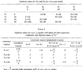
Algebraic values f o r Pls and Fls for a two-gene model.

-~ _-

p1 pz Pa P*

0 2d 2d 4d

. . . _ ~ _ _ _ _ _ _ ~ -

PI 0 d+dh d+dh 2df2dh

pz 2d d+dh 2d+2dh 3d+dh

p3 2d d+dh 2d+2dh 3dfdh

P4 4d 2d+2dh 3d+dh 3dfdh

TABLE 4

Algebraic valuesfor c.p.r.’s, together with valuesfor these regression coeficients with diferent values of “h.”

_____

CONSTANT PARENT REGRESSION VALUES

CONSTANT

n < - 1 OR

.. . . . - -. _. . -

h’+l OR h = - l

ALGEBRAIC

VALUES h = + l h=l+a.a>O h=a-l.a<O

PARENT h=O

a 2 l + h

P1=0

__

Pz = 2d . 5 .5 .5 . 5 . 5 . 5

P3=2d . 5 .5 .5 .5 . 5 .5 .5 1

.o

l+A

0

+-

2 2

. 5 0

h

4d

308 BRUCE GRIFFING

2. Both dominance and epistasis

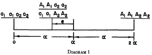
I n setting up this model we may regard diagrammatically epistasis as an interaction between loci analogous t o dominance as an interaction between alleles a t the same locus. The basic diagram is the following which shows the four parental values.

A1 AI a2 02

01 01 o2ag 01 a, A,*, AI AI A2 A2

+a--+--a--l

- e

I

0

a

2 a

DIAGRAM 1

The genotypic values for the heterozygotes may be obtained by the fact that the f is a dominance deviation away from the midpoint between its homozygotes. For example, the following diagram shows the derivation of

A 1ma2a2.

Alalapa2 = 1/2(1

-

e)(l

+

h)a.

Following such a scheme all P I and F1 values may be established, and the algebraic values are given in table 5.

TABLE 5

Algebraic values for PIS and Fis involving both dominance and epistasis.

PI p2 PI PI

0 a(1-e) a ( l -e) 2a

A i A i A z Az

--

aiel A2 A2

-__ A d i m m

-___ aialmaz

a a U

- (1-e+h-eh) - (1-e+h-eh) - (2-e+2h+ehz)

2 2 2

P1=0

a a

- (2-e+2h+eha) .? (3-efhfeh)

2 2

Pz=a(l-e) - (1-e+h-eh) 2

a a a

- (3--e+h+eh) 2

PI=a(l-e) - (1-e+h-eh) - (2-e+2h+eh2)

2 2

a a U

- (2-e+2h+ehP) - (3-e+h+eh)

QUANTITATIVE GENE ACTION 309 TABLE 6

Algebraic values for c.p.7. coe$cients for both dominance and epistasis.

CONSTANT PARENT c.p.r. COEFFICIENTS

P1=0

Pz=a(l-e)

9 - 2eh(2eh - 3)

1 { (1 -h) -e[(l -h)*+eh(l -h)] )

2 (l-e)z

Pa=a(I -e) bp3 = - - 6 F + F

--__

I-’4 = 2a bp4=- -

Using these algebraic values, c.p.r. coefficients may be calculated for each c.p. group, and these are listed in table 6.

It may be noted from tables 5 and 6 that if “e” is equated to zero, then all algebraic values reduce to those in the first model (letting a = 2 d ) .

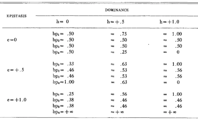
A two-way classification table may be constructed to demonstrate the trends of c.p.r. coefficients for different numerical values of “e” and “h.” These values are found in table 7.

The following characteristics of the “e” by “h” table may be noted. (1) When e=O, h=O, bpi=.5, as found earlier.

(2) When e=O, and “h” varied (first row), the same trend occurs as found in table 4, which is a steadily decreasing regression trend from bp, to bpl. The relative decrease depends on the degree of dominance.

TABLE 7

Two-way classification of various values of “e” and “h” for

constant parent regression coeficients.

_____ -

-

DOMINANCE

-_

EPISTASIS

h = 0 h = + . 5 h = + 1 . 0 = .75

=

.so

=

.so

= .25

= .63

= .53

= .53

= .63

= .56

= .46

= .46

= + w

= 1.00 =

.so

=

.so

=

o

= 1.00 = .56 = .56

=

o

= 1.00 = ’46

= .46

310 BRUCE GRlFFING

(3) When h=O, and “e” varied (first column), epistasis is considered alone .

without the confounding influence of dominance. The regression trend is opposite to that of dominance alone, as the regression trend steadily increases from bpl to bp,. The relative increase depends on the degree of epis tasis.

(4) When “h” and “e” both have values other than zero--i.e., e = +.5,

h = +S-then conflicting regression trends result in a decrease from bpl to bpz and an increase from bp3 to bpd.

A consideration of RASMUSSON’S (1933) interaction hypothesis can be made by merely assigning “e” negative values. The hypothesis may be summarized by stating that the phenotypic result of the addition of genes follows the law of diminishing returns. I n other words, genes added when the character expres- sion is low would have much greater effect than when the character expression is near a physiological limit.

The above two-gene pair model is only one of many possible approaches to between-loci interaction. It is an attempt to combine in one model both dominance and epistatic effects and still allow algebraic solution. An extension of this model to more gene pairs may be difficult and for an extended epistatic and dominance model the logarithmic case is chosen and will be discussed later.

HULL (1947a) has presented a regression equation which involves both dominance and complementary gene action.

BURDICK (1949) has developed an epistatic model for multiplicative effects of gene pairs assuming no dominance. The c.p.r.s yield an increasing trend in much the same manner as the epistatic model described above with h=O. Testing for significance of bz (in both models) by an ordinary analysis of variance for the regression of c.p.r. coefficients on parental values is not valid because the c.p.r. coefficients are highly correlated. The problem can be ap- proached by fitting constants to the following regression equation by least squares procedure:

Fij = m

+

al(Pi

+

Pj)

+

az(Pi2

+

Pj2)

+

a3(PiPj)

+

eij

i.e. by estimating and testing al, a2, and 93. Because a3 is equal to bz for the case of dominance alone, a test of significance of a3 is equivalent to a test of significance for b2 for dominance alone. Similarly since a2 approximates b2 for the case of epistasis alone (for the two-gene-pair model) a test of signifi- cance for a2 is equivalent to a test for bz for epistasis alone. When “e” and “h” both have some value, the c.p.r. trend is curvilinear with respect to c.p. values

so that the regression coefficient bz would have little meaning. B. Extension of two-gene-pair models

1. Dominance but no epistasis Model specifications are as follows:

1. There are “n” loci affecting the specified character.

311

3. Effects of genes a t different loci are additive.

With “n” loci and the alternative of two alleles a t any one locus, there are 2” number of different possible homozygous parental lines. These inbreds may be denoted simply by their gamete arrangement, and all possible gamete ar- rangements may be indicated merely by the expansion of

fi

(Ai

+

ai).

i=l

Parents of different genotypic constitution may have the same genotypic value, and thus Fls with different genotypic values may result from crosses in which the parents have the same genotypic values. For example, from the three- gene-pair case as illustrated in table 8, one can see that parent No. 6 (AluzA3)

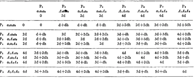
TABLE 8

Algebraic valuesfor all possible parents and Fls involved in the three-gene-pair model.

PI Pa Pi P. PS Pa P7 PI

a ~ a m Atallla aiAxzs ara,Aa AIAIat A a A a a ~ A d i AiAzAa

0 2d 2d 2d 4d 4d 4d 6d

-

PI alaPat 0 0 d t d h d+dh d+dh 2dfZdh 2d+2dh Zd+Zdh 3 d t 3 d h

PI Alaai 2d d t d h 2d 2df2dh Id+Zdh 3dfdh 3dfdh 3d+3dh 4d+2dh PI alArar Zd d f d h Zd+Zdh 2d 2df2dh 3 d S d h 3d+3dh S d f d h 4d+2dh P, alarAl 2d d f d h 2df2dh 2dS2dh 2d 3d+3dh 3d+dh 3d+dh 4df2dh

PS AIAlaa 4d 2df2dh 3d+dh 3d+dh 3d+3dh 4d 4df2dh 4dS2dh Sdfdh

Ps AlalAa 4d 2d+ldh 3d+dh 3dS3dh 3 d S d h 4d+2dh 4d 4d+2dh Sd+dh Pi alAIAt 4d 2dfZdh 3df3dh 3dfdh 3d+dh 4dfZdh 4 d f 2 d h 4d Sd+dh

P S AlAsAs 6d 3d+3dh 4dS2dh 4dS2dh 4df2dh 5d+dh Sdfdh SdSdh 6d

has a value of 4d, and parents No. 4 (Al~za3) and No. 3 ( ~ 1 A z ~ 3 ) both have val

ues of 2d. However, the F1 ( 6 x 4 ) =3d+dh, and the FI ( 6 x 3 ) has a different value namely, 3d+3dh. Therefore, it is impossible to determine uniquely the F1 genotypic value with knowledge of only the parental genotypic values. In other words, in the three-dimensional coordinate system, where Pi, Pj and Fij are the three axes, a three-dimensional constellation of points would be generated with “n” gene pairs rather than a simple surface (if the measure- ments used were the genotypic values).

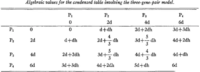
312 BRUCE GRIFFING TABLE 9

Algebraic valuesfor the condensed table involving the three-gene-pair model.

PI Pz Pa P4

0 2d 4d 6d

p1 0 0 d+dh 2d+2dh 3d-h-

4d+2dh

4d+dh

4 5

d+dh 2d+- dh 3d+- dh

3 3

4 4d+- dh 5

3 3

pz 2d

P3 4d

p4 6d 3d+3dh 4d+2dh 5d+dh 6d

2d+2dh 3d+- dh

each parental genotypic value. The F1 values in table 9 are averages and may be obtained in two ways.

1. The F1 values in table 8 may be averaged in the manner described above. 2. HULL (1946, 1947) suggests the following general scheme for determining Let U and w be the proportion of A A loci in Pi and Pj, respectively, and (1 -U) and (1

-

w) be the proportion of aa loci. The average F1 value may be determined as follows:

the genotypic value for any particular F1 cell of table 9.

Pi gametes

Y

A U

U 1 - U Parental coded values are:

A w uw w(1-U)

Pi

P i = u 2nd

gametes Pj = w 2nd

a 1-w u(1-w) (1-u)(l-w) Then

Fij = ~ ~ ( 2 n d )

+

( w ( 1

-

U)

+

u ( l

-

w))n(d

+

dh). (1) (Parental and F1 values are coded so that the completely recessive genotype, alala2a2 + anan, has a genotypic value of zero.)

With HULL’S theoretical procedure a regression surface is fitted to the three- dimensional scatter, and equation (1) may be used to predict the exact average

F1 values found in the cells of table 9.

QUANTITATIVE GENE ACTION 313 To illustrate this point, one may first re-write equation (1) in terms of pa- rental values and then partially differentiate the F1 with respect to the variable parent.

Pi

+

Pj h

F.. 1 J - -

-

(1

+

h) - - PiPj.

2 2nd

The rate of change in the Fij with change in P j (variable parent) and con-

sidering Pi as the constant parent may be expressed as follows: dFij 1

+

h h

- -

_{Pi = bpi (c.p.r. for Pi).}

dP j 2 2nd

The second order regression coefficient, which represents the rate of change in bpi with change in the constant parent (Pi), may be represented as follows:

h - bz. -

dbpi

d P i 2nd

However, in practice where, obviously, only a sample of all possible parental genotypes can be used one is not confronted with the idealized regression sur- face but rather the actual Fl scatter. Under such conditions the c.p.r. scheme is not exact. This may be illustrated by forming different sets of parents in

CP = 0 CP = 2 d

0 2 d 46 6 d VARIABLE PARENT

0 1

0 2d 4 d 6 d VARIABLE PARENT

CP = 4 d CP: 6d

00

0 2d 4 d 6d VARIABLE PARENT

2d

t

0

-0 2d 4 d 6 d VARIABLE PARENT

3 14 BRUCE GRIFFING

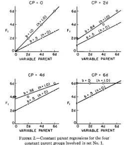
which no one set contains all possible parents. From the three-gene-model, let us consider two parental sets ($=PI, P2, P5, P8 and S2=P1, Pq, P6, P8) chosen from table 8. Figures 2 and 3 give the c.p.r.’s for

S1

and

SZ

respectively for the condition of complete dominance. The no-dominance (h = 0) regressions for each c.p. group are also included. Table 10 gives algebraic values for c.p.r. coefficients, variances of Fls, and other statistics for the three sets, SI,

SZ,

and the condensed (ideal) set. It is obvious that the regression trends in all three sets reflect the dominance effect when “h” takes on some value other than zero. Although the same “h” value may be assigned to all three sets, the correspond-

C P = 0 CP = 2 d

VARIABLE P A R E N l

CP = 4 d

0 2d 4d 6d

VARIABLE PARENT

0 2d 4d. 6 d VARIABLE PARENT

C P = 6 d

Fl

0 2d 4 d 6 d VARIABLE PARENT

FIGURE 2.-Constant parent regressions for the four constant parent groups involved in set No. 1.

ing c.p.r. coefficients do not exactly agree. Thus, because of the sampling pro- cedure operating in obtaining the set of parents, the c.p.r.’s do not exactly reflect the magnitude of dominance, although the inexactitude would probably be small if a wide range of character expression is exhibited among the parents. However, the fact thatsone has to deal with unpredictable points in the F1

scatter, although causing some irregularities in the practical use of the c.p.r. technique, does offer another approach to the problem of dominance estima- tion.

QUANTITATIVE G E N E ACTION 315

3

I

0

m

3

+

0

T

-9

0

3

h

3

x

₊

$

I Eb

II

d

316 BRUCE GRIFFING

GP = 0

6 d

4 d

Fl

.

2 d

0

VARIABLE PARENT

0 2d 4 d 6 d VARIABLE PARENT

G P = 2d

0 2d 4 d 6 d VARIABLE PARENT

GP = 6 d

0 2d 4 d 6 d VARIABLE PARENT

FIGURE 3.-Constant parent regressions for the four constant parent groups involved in set No. 2

homozygous parents and controlled matings a slightly different mathematical model may be used. The genotypic value of an FI is composed of two parts, a basic gene effect which is a function of “d,” and a dominance effect which is a function of “dh.” The variance among Fls then involves a basic gene vari- ance, a dominance variance, and a covariance, as these two effects may be correlated (see table 10). The partitioning of variances will be discussed after the next section.

2. Both dominance and epistasis (logarithmic case)

There are undoubtedly many ways that interaction between loci can be handled. The only general scheme that will be mentioned here will be that resulting from logarithmic gene action. When characters controlled by logarith- mic or geometric gene action are measured in arithmetic values, it is obvious that gene interaction exists. I n other words, the addition of a gene has an exponential or multiplicative effect, the value of which depends not only on its own activity but also on the presence of other genes in the genotype. By working out simple numerical examples, it may be readily observed that this general type of interaction as expressed on the arithmetic scale is detected by an increasing regression trend similar to that in the epistatic two-gene-pair model.

QUANTITATIVE GENE ACTION 317 itself is transformed to the additive scheme and the interaction disappears. This type of interaction is termed metrical bias and results when variations are measured on a different scale than is actually involved in the growth and expression of the character.

The problem then is first to choose whether the arithmetic or logarithmic scale will yield the best fitting model. This is taken up in the last section which discusses the general procedure for fitting gene models.

PARTITIONING OF VARIANCE OF Fls WITHIK A CONSTANT PARENT GROUP

Let us assume that the proper transformation has been made so that be- tween-loci effects as well as environmental effects are additive and independent. Consider, then, the ith constant parent group, which has CP; as the constant parent, VPjs where j = 1, 2,

. .

.,

n (i#j) as variable parents, and Fijs are Fls resulting by crossing CPi on all other variable parents.

The mathematical models involved are as follows: CPi = gi

+

ei

VPj = gj

+

ej

(where MPij is the midparent between CPi and VPj) <:Pi, VPj, Fij and MPij represent the phenotypic measurements for the

particular trait considered on the ith constant parent (CPi), the jth variable parent (VPj), etc. gi is the basic gene effect, which, in the gene model, is a function of “d” only. ei, eij are individual errors. hij is the dominance effect for the Fij and is a function of “dh” only.

TJsing the above mentioned models the Fijs of the ith constant parent group, associated variable parents and midparents may be represented as follows:

Fij VPj MPij

-

gi gz gi g z ei e2

MPi2 = -

+

-

+

-

+

-

2 2 2 2

2 2

Fi2 = -

+

-

+

hi2

+

eiz VP2 = g2

+

e2

gi gn gi g, ei en

MPin = -

+

-

+

-

+

-

2 2 2 2 2 2

Fin = -

+

-

+

hin

+

ei, VP, = gn

+

en where i#j.

and covariances.

318 BRUCE GRIFFING -

E(gk-E.)=E(hij-hi.)=E(e,)=O where k = i or j ; m = i , j or ij E(gk -

E.)

= ag2; E(hij -hi.) = a h 2 ; E (em2) = ae2

E(gk--g.)(hik-%i.) =PQg'Jh, expected values of all other cross-products are

zero.

g.

is the mean genotypic value of the parents.

hi. is the mean dominance value of the Fa in the itl1 c.p. group.

The problem is to partition the variance of Fls within each constant parent group and estimate the variances ug2 and a h 2 , and the correlation p . The variances and covariances are denoted as follows:

~-

V ( F ~ ~ ) =variance of the F1s within the ith c.p. group.

V(VP, =variance of the variable parent values in the ith c.p. group. V(MP) =variance of midparental values of the variable parents and the

V ( F ~ - M P ) =variance of the differences between the F1s and their correspond-

C V ( F ~ X V P ) =covariance of the Fls and their corresponding variable parents. constant parent.

ing midparents.

The expected values of these variances and covariances are as follows: E

{

V(Fij)

}

= ( i ) . g 2

f

'Jh2

+

Pagah

+

a e 2 E

{

V(F1-MP)

1

= a h 2

+

(8)ae2 E ( V(VP)

]

= ag2

+

ae2

E

{

v ( M P ) ) = (+>ag2

+

(3>ae2 E

{

C V ( F ~ X V P )

]

= (&)flg2

+

P'Jgah-

Estimates of the genotypic components are obtained by equating observed and expected values.

/ \

( t ) $ g 2 = 1/41 (VVP - ke2)

]

p u g a h = V ( F i j )

-

($)8g2

-

&h2

-

&e2 8 h 2 = V(F1-MP)

-

( * ) b e 2 .

The error component ae2 is directly estimated from the analysis of variance of the replicated experiment and is the variance of parental and Fl means (experimental error variance divided by the number of observations per parent or FI).

The genotypic c.p.r. coefficient is:

where PhXg is the regression of the dominance contributions on the parental values.

These expected c.p.r. coefficients are estimated by:

QUANTITATIVE GENE ACTION 319

from the constant parent regression. Thus, the separation of the F1 variance into (1) the portion attributable to regression and ( 2 ) the portion due to devia- tions from regression, is of considerable importance as an aid in identifying the best fitting model. It is also of interest to point out the relationship existing between these portions and the components of the F1 variance which have previously been discussed, namely ug2, a h 2 and PUgUh. I n terms of components

the expected genotypic fraction of an F1 variance attributable to the c.p.r. is as follows:

and the expected fraction due to deviations from regression is: (1 - p2)Uh2.

It is obvious that if p = O then the basic gene variance and the mean square attributable to regression are equivalent; also the dominance component and deviations from regression are identical. If p f O this relationship does not hold. I n the gene model in which dominance exists but no between-loci-interaction, and all of the dominance effects are in the same direction of character expres- sion, one can use variance components to estimate the value of “h.” This necessitates theoretically the inclusion among the set of parents, of a complete- ly recessive or completely dominant inbred or both. Then with their c.p. groups the dominance

estimated as follows:

value to be associated with the gene model may be

Overdominance is indicated when a h 2 is greater than

ag2.

following F test;

Tests of significance for the dominance component may be obtained by the

with (n- 1) degrees of freedom for the numerator where “n7’ is the number of Fls in the c.p. group, and degrees of freedom for the denominator equal the degrees of freedom on which the experimental variance is based.

USE O F P O T E N C E RATIOS $OR CALCULATING APPROXIMATE MAGNITUDE O F DOMINAKCE

In addition to the use of regression trends and variance component analyses, one can approximate a dominance value from the means of the non-segregating populations.

320 BRUCE GRIFFING

the F1 means with mid-parental values to determine a “potence” value (h,) as follows:

Fi

-

Mp

I

p

-

MPI

where: M, = midparent h, =

P = parent (extreme) This potence value will sufficiently approximate an average dominance value for the models discussed if one of the parents is a t either extreme of character expression.

GENERAL PROCEDURE FOR FITTING G E N E MODELS

The following steps are listed as the general procedure which may be used 1. From arithmetic P1 and F1 means various statistics are calculated, such as (a) c.p.r. coefficients, (b) variance components, (c) deviations from the c.p.r., and (d) h, values for the Fls.

2. If the regression trend is decreasing, then positive dominance is assumed with arithmetic gene action. Amount of dominance is estimated by severity of regression trend, components, and h, values.

3. If the regression trend is increasing, then the first problem arising is to distinguish between,. (1) arithmetically cumulative action with negative dominance, and (2) logarithmically cumulative gene action with or with- out dominance.

This may be done by transforming the data to logarithms and comparing (1) If on transformation to logarithms the c.p.r. trend is drastically reduced in comparison with the trend of the arithmetic c.p.r.s, this indicates that the arithmetic trend is due to logarithmic interaction (metrical bias) which can be removed by transformation.

(2) If on transformation to logarithms the deviations from regression are greatly reduced, this indicates that the deviations from regression are due mostly to metrical bias which disappears with transformation, and the best model would involve the logarithmic scale.

(3) If h, values are irregular with arithmetic data and on transformation to logarithms become much more uniform, then this indicates that the better gene model is logarithmic.

(4) If in arithmetic analysis the c.p.r.s are all positive but increase sharply with largest valued c.p.r. considerably over

+

1.0, then this indicates logarithmic gene action. With negative dominance the c.p.r. coefficients should never exceed

+

1.0 (disregarding’ errors associated with c.p.r.’s) except in the case of overdominance, and usually one c.p.r. should have

a negative value.

These four criteria may be used effectively to differentiate logarithmic from arithmetic gene action. When the proper basic gene action is decided upon, then estimates of amount of dominance are obtained by using the appropriate data (arithmetic or logarithmic) from the following statistics, (a) bz, severity of regression trend, (b) components of variance, and (c) h, values.

to fit the data to a specific gene model.

QUANTITATIVE GENE ACTION 321 The development of the c.p.r. technique is obviously in its preliminary stages. However, when the trends of c.p.r. coefficients are used in combination with other approaches, a satisfactory analysis of the average gene action may be obtained. It should be emphasized again that as wide a range of character expression as possible is desirable. At least one extreme or both should be iiicluded among the parents so that regression trends, potence and component ratios are more reliable.

The real test of a new technique is in its practical application. HULL (1948) has reported some results in corn. Probably the most extensive use has been in the analysis of some ten characteristics in tomatoes (GRIFFING 1948). Here considerable success was obtained in fitting gene models to the data by the techniques outlined in this paper.

SUMMARY

An approach to the analysis of quantitative inheritance by use of the con- stant parent regression method is outlined. Variance components are also considered as an aid in understanding the relation between constant parent regressions and dominance deviations, and in evaluating the magnitude of dominance.

The approach is essentially that of constructing different gene models and then choosing the model that fits the data most accurately as determined by various statistics. As an introduction to the techniques, two-gene-pair models are considered first involving (1) additive gene action with dominance and no epistasis, and (2) gene-interaction involving both dominance and epistasis. The models are extended to “n” gene pairs with logarithmic gene action being the only type of gene interaction discussed. A procedure for differentiating the two basic models, arithmetic and logarithmic, is outlined together with an estimation of the amount of dominance on the closest fitting scale.

ACKNOWLEDGEMENTS

The author is indebted to DRS. JOHN W. GOWEN, SEWALL WRIGHT, and FRED H. HULL for constructive criticisms of the manuscript and to PROFESSOR OSCAR KEMPTHORNE for valuable aid in the statistical aspects of the paper.

LITERATURE CITED HURDICK, A. B., 1949

FISHER, R. A., 1918 GRIFFING, J. B., 1948

HULL, F. H., 1946 Maize Genetics Cooperation News Letter 20.

Heterosis in the tomato; estimation of the relative contribution of epistasis The correlation between relatives, on the supposition of Mendelian in- Statistical analysis of gene action in components of tomato yield. Un- and dominance. Unpublished Ph.D Dissertation, University of California.

heritance. Trans. roy. Soc. Edinb. 52: 399-433.

published Ph.D Dissertation, Ames, Iowa State College, Ames, Iowa.

1947a Theoretical regrezsion of F, on homozygous parents with additive or complementary gene action. Genetics 32: 9G91.

1947b Maize Genetics Cooperation News Letter 21. 1948 Maize Genetics Cooperation News Letter 22.

MATHER, K., 1949 Biometrical Genetics, pp. 82-97. Dover Publ. Inc., London.