ABSTRACT
THOMPSON, KARMETHIA CHANTAL. Solving Nonlinear Constrained Optimization Time Delay Systems with a Direct Transcription Approach. (Under the direction of Dr. Stephen L. Campbell.)
In this thesis we explore the application of SOCX, a direct transcription (DT) optimization software tool that employs Runge-Kutta methods and interpolating polynomials for the solu-tions to nonlinear constrained optimal control systems containing both state delays and control delays. Direct transcription methods are popular direct methods that in some form transcribe the entire optimal control system into a large sparse nonlinear programming problem (NLP) by some discretization scheme. Optimal control delay solvers are important because they help to provide numerical solutions to large time delay ordinary differential equations (ODEs) or differential algebraic equations (DAEs), optimal control problems (OCPs), and other optimiza-tion systems that describe modeled processes that commonly arise in research and industry.
added weighting factor tends to zero in the cost function.
©Copyright 2014 by Karmethia Chantal Thompson
Solving Nonlinear Constrained Optimization Time Delay Systems with a Direct Transcription Approach
by
Karmethia Chantal Thompson
A dissertation submitted to the Graduate Faculty of North Carolina State University
in partial fulfillment of the requirements for the Degree of
Doctor of Philosophy
Applied Mathematics
Raleigh, North Carolina 2014
APPROVED BY:
Dr. Hien Tran Dr. Negash Medhen
Dr. John T. Betts Dr. Stephen L. Campbell
DEDICATION
This thesis is dedicated to the living memories of my aunt, Earlene Lambry. I truly wish that you could have been here to experience this moment with me. I hold my head high knowing
BIOGRAPHY
Karmethia Thompson was born in Atlanta, GA on April 5, 1986 to parents Catherine Hall and Leon Thompson. She is the middle child with two sisters, Sophia Hall and Kanisha Thompson. She grew up in the East Atlanta community and graduated in 2004 from Southside Comprehen-sive High School. Throughout her high school years she participated in a variety of activities: basketball, softball, soccer, and band. However, it was her love for math that opened doors to college opportunities. She graduated from the “GREAT” Bethune-Cookman University in 2008 with a B.S. in mathematics with a concentration in computer science.
While in college she was a member of the Florida-Georgia Louis Stokes for Minority Par-ticipation program (FGLSAMP), an academic support program that provides counseling, men-toring, tutoring and shadowing services to minorities in an effort to encourage them to pursue careers in Science, Technology, Engineering, and Mathematics (STEM). This program gave her exposure to opportunities beyond college. After graduating college Karmethia moved to Raleigh, NC where she attended graduate school at North Carolina State University.
ACKNOWLEDGEMENTS
This research was in part funded by the National Science Foundation under NSF Grant DMS-1209251.
I am especially grateful for having Dr. Stephen Campbell, committee chairman as my advisor. His knowledge, expertise, passion, and guidance help to facilitate this entire process. His sup-port and encouragement pushed me to work harder in those trying times. Under Dr. Campbell’s direction I have learned many things such as optimal control, professorship, writing skills, and even a few stories about the lessons of life. For these skills acquired I am forever thankful.
Additionally, I wish to thank a few of the faculty and staff at North Carolina State Uni-versity. Special thanks to my committee members Dr. Medhin, Dr. Tran, and Dr. Betts who were more than generous with their expertise, feedback, and precious time. I would like to emphasize that Dr. Betts is a distant committee member and made several trips across the country to support my degree process. I thank him for his commitment and support. To Ms. Denise Seabrooks, Mathematics Department Graduate Service Coordinator, I thank you for the outstanding service that you have given the graduate math department. Your efforts are always filled with love and sincerity. Without your hard work I would have forfeited my preliminary exam. This is just one of the many occasions that you saved me. Thank you so much! NC State you prepared a big stage for me to perform on. Thanks for giving me the support needed to rise to the occasion.
It would not have been possible to write this doctoral thesis without the help and support of my fellow colleagues. I wholeheartedly thank Ms. Nakeya Williams and Mr. Terrance Pendleton for their friendship and support. I could always rely on you anytime of the day and any hour of the night. I am sure that we will remain friends throughout our careers. I wish each of you the best. Special thanks to LaKendra Blash for helping me prepare for my seminar and conference presentations. Your advice and criticism was greatly appreciated.
mentors Mr. Demarco Mitchell and Mrs. Annette Alexander, I thank you for challenging me to be the best student I could be. It was your faith and encouragement that inspired me to pursue a higher education degree. To my grandmother, Idell Lambry, you are my rock. Thank you for your strength. To my mother and father, Catherine Hall and Leon Thompson, you are the roots that keep me focused and grounded. All that I have achieved and all that I will accomplish is for you.
TABLE OF CONTENTS
LIST OF TABLES . . . viii
LIST OF FIGURES . . . ix
Chapter 1 Background: The Optimal Control Problem . . . 1
1.0.1 Problem Description . . . 2
1.0.2 Pontryagin’s Minimum Principle . . . 4
Chapter 2 Introduction . . . 6
2.1 Motivation . . . 6
2.2 Optimal Control Delay Systems . . . 8
2.2.1 Facts About Delays . . . 12
2.3 Time Delay Software and Optimization Tools . . . 16
2.3.1 Delay Differential Equation Numerical Techniques . . . 17
2.3.2 Optimal Control Numerical techniques . . . 18
2.4 Dissertation Outline . . . 20
Chapter 3 Direct Transcription and Software . . . 24
3.1 Direct Transcription . . . 24
3.2 Sparse Optimal Control Extended . . . 28
3.2.1 SOCXAlgorithm . . . 30
3.2.2 Test Problems . . . 35
Chapter 4 Exogenous Input Control Method . . . 54
4.1 Control Delay Optimization Problems on Nonuniform Grids . . . 54
4.1.1 Simple Mixed Delay Problem . . . 55
4.1.2 Nonuniform Grids are Necessary . . . 64
4.2 Exogenous Input Control Method . . . 64
4.2.1 Control Delay Test Problems Resolved with the EIC Method . . . 67
4.2.2 Results Summary . . . 76
Chapter 5 Analysis and Convergence of EIC. . . 86
5.1 Method of Steps Approach . . . 88
5.1.1 OMOS: PMP applied to the MOS formulation for (5.1) . . . 89
5.1.2 EMOS: PMP applied to the MOS formulation for (5.2) . . . 91
5.1.3 Results Summary for OMOS and EMOS . . . 94
5.1.4 A Special Consequence of the Exogenous Input Control Method . . . . 97
5.2 εAsymptotic Approximation Approach . . . 99
5.2.1 An Asymptotic Solution to the EIC Test Problem . . . 101
5.2.2 A Reduced Form of the Asymptotic Solution to URTP . . . 105
Chapter 6 SOCX, DAEs, and More General Delay Problems . . . 119
6.1 Advanced Time Systems . . . 120
6.2 Mixed-type Delay Systems . . . 124
6.3 Neutral Delay Systems . . . 125
6.4 Time-Varying Delay Systems . . . 127
Chapter 7 Conclusion . . . 130
7.1 Future Work . . . 133
Chapter 8 Contributions of Thesis . . . 140
8.1 Papers . . . 140
8.2 Presentations . . . 143
REFERENCES . . . 144
Appendices . . . 153
Appendix A SupportingSOCXFiles . . . 154
A.1 Driver for Optimal Control Delay Problem . . . 154
A.2 Matlab Files for Graphing SOCXOutput . . . 171
A.2.1 Code for Standard Optimization Problems . . . 171
A.2.2 Code for Method of Steps Problems . . . 176
Appendix B Analytic Solution for the Control Delay Problem . . . 180
LIST OF TABLES
Table 3.1 Estimated absolute max errors for IR in Eq. (3.9) . . . 39
Table 3.2 Solution comparison for IR in Eq. (3.9) . . . 40
Table 3.3 Control delay problem solution comparison . . . 43
Table 3.4 Eq. (3.11) Estimated max errors . . . 47
Table 3.5 CSTR problem solution comparison . . . 48
Table 3.6 Eq. (3.12) Max Error Order . . . 53
Table 4.1 Sample grid refinement for (4.1) . . . 58
Table 4.2 Delay time values applied to Grid 2 mesh . . . 58
Table 4.3 Max errors for ECDP in Eq. (4.4) computed at ε . . . 70
Table 4.4 Optimal control summary for ECDP in Eq. (4.4) . . . 71
Table 4.5 Max errors for ESMD problem in Eq. (4.5) computed atε . . . 74
Table 4.6 Max errors for CSTR in Eq. (4.6) computed at ε . . . 76
Table 5.1 J∗(ε): Performance index for (5.17) . . . . 115
Table A.1 Standard Optimal Control Analysis Grid for Eq. (4.1) . . . 171
LIST OF FIGURES
Figure 2.1 State Delay Problem: Eq. (2.9) solved withq = 1 . . . 13
Figure 3.1 Sample discrete time grid after subdivision on an interval [tI, T] . . . 24
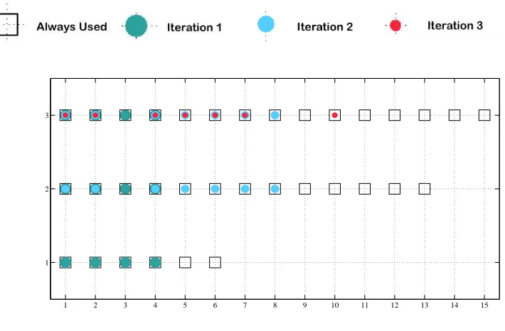
Figure 3.2 Master legend for graphs featured in Chapter 3 . . . 36
Figure 3.3 MOS solution for IR in Eq. (3.9) . . . 38
Figure 3.4 SOCXsolution for IR in Eq. (3.9) . . . 38
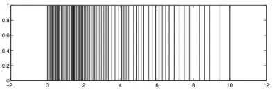
Figure 3.5 Bar graph representation of final time grid for IR in Eq. (3.9) . . . 39
Figure 3.6 MOS solution for the control delay problem in Eq. (3.10) . . . 41
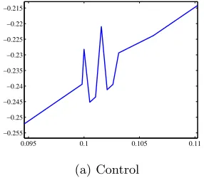
Figure 3.7 Final iteration SOCXsolution for the control delay problem in Eq. (3.10) . 42 Figure 3.8 Close-up of control for the control delay problem in Eq. (3.10) . . . 42
Figure 3.9 Iteration 1SOCXsolution for the control delay problem in Eq. (3.10) . . . 42
Figure 3.10 MOS solution for the CSTR problem in Eq. (3.11) . . . 45
Figure 3.11 Iteration 1SOCXsolution for the CSTR problem in Eq. (3.11) . . . 45
Figure 3.12 Iteration 5SOCXsolution for the CSTR problem in Eq. (3.11) . . . 46
Figure 3.13 Final Iteration SOCXsolution for the CSTR problem in Eq. (3.11) . . . 47
Figure 3.14 Graphical representation of the evaluation of the delayed state variable . . 50
Figure 3.15 Case 1 for Eq. (3.12) . . . 51
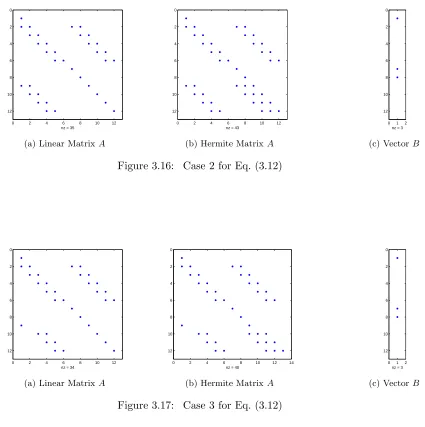
Figure 3.16 Case 2 for Eq. (3.12) . . . 52
Figure 3.17 Case 3 for Eq. (3.12) . . . 52
Figure 4.1 MOS Solution for SMD in (4.1) . . . 56
Figure 4.2 SOCXsolutions for SMD in Eq. (4.1) . . . 57
Figure 4.2 SOCXsolutions for SMD in Eq. (4.1) continued . . . 58
Figure 4.3 SOCXresults for Eq. (4.1) solved on Grid 2 . . . 61
Figure 4.4 Grid points utilized during interpolation on Grid 2 for Eq. (4.1) . . . 62
Figure 4.5 SOCXsolution with chattery control on a fine nonuniform grid for (4.1) . . 63
Figure 4.6 Final iteration for ECDP in Eq. (4.4),ε = 1.0E-06 . . . 69
Figure 4.7 Regularized control in Eq. (4.4) forε= 1.0E-06 vs. original control in Eq. (3.3) 70 Figure 4.8 Final iteration for ESMD problem in Eq. (4.5),ε=1.0E-04 . . . 72
Figure 4.9 Closeup of the regularized control for ESMD problem in Eq. (4.5) . . . 73
Figure 4.10 Final iteration for ECSTR problem in Eq. (4.6), ε= 1.0E-08 . . . 76
Figure 4.11 Closeup of regularized control in Eq. (4.4) . . . 77
Figure 4.12 Iteration 1: Solutions for (4.8), ε= 10−4 . . . . 81
Figure 4.13 Iteration 2: Solutions for (4.8), ε= 10−4 . . . . 82
Figure 4.14 Iteration 3: Solutions for (4.8), ε= 10−4 . . . 83
Figure 4.15 MOS exogenous controls for test problems . . . 84
Figure 5.1 OMOS Solution . . . 95
Figure 5.2 EMOS Solution . . . 96
Figure 5.3 Jump Discontinuity in λ2ε(t) at t= 4 . . . 97
Figure 5.4 Delta function depiction of (5.14) . . . 105
Figure 6.1 Evolutionary method optimal solutions for Eq. (6.1) . . . 122
Figure 6.2 SOCXsolution for the ADE problem in Eq. (6.2) . . . 123
Figure 6.3 SOCXfinal grid for Eq. (6.2) . . . 123
Figure 6.4 SOCXsolution for MTD problem in Eq. (6.3) . . . 124
Figure 6.5 Final grid for MTD problem in Eq. (6.3) . . . 125
Figure 6.6 SOCXsolutions for NDE problem in Eq. (6.5) . . . 127
Figure 6.7 Matlab MOS and SOCXsolutions and error for Eq. (6.5) plotted on [0, 1.5] 128 Figure 6.8 SOCXsolutions for TVD problem in Eq. (6.6) . . . 129
Chapter 1
Background: The Optimal Control
Problem
Optimal control theory is a mathematical discipline that focuses on finding optimal ways to control a dynamic system. It is an extension of the calculus of variations, a branch of mathemat-ics concerning problems that seek to find the path, curve, or surface for which a given function has a minimum or maximum. Let [t0, t1] be a fixed time interval, then a simple calculations of
variations problem minimizes the integral functional
J =
Z t1
t0
F[x(t),x(t), t]˙ dt, (1.1a)
over the curvesx(t) : [t0, t1]→Rm satisfying the conditions
x(t0) = ˆx(t0), x(t1) = ˆx(t1), [x(t)T,x(t)˙ T, t]∈ Q a.e. on [t0, tf], (1.1b)
where ˆx0, ˆx1 ∈ Rm are certain fixed points,Q ⊂ R2m+1 is an open set, and F : Q → R1 is a
1.0.1 Problem Description
Optimal control theory studies similar problems but from a more dynamic perspective. A typical problem in optimal control theory involves a system that is composed of a set of differential equations that represent the propagation of the differential or state variables as a function of the independent variable, say, time [131]. The components of the state vector may reflect position, velocity, acceleration, or other physical properties and are impacted by the presence of an input variable termed the control. In practice, many optimal control problems impose restrictive conditions orconstraintson both the state and the control. Constraints are broken up into two main categories,path constraintsorpoint constraints. Path constraints restrict the range of values taken by either the state, control, or both variables over the entire time interval, [t0, t1], or any time subinterval. Point constraints are usually imposed asboundary
constraintswhich require the system’s response to achieve a given target at a specific terminal time,t1or initial timet0. Constraints can be better explained through the following example.
Consider a dynamical system that wishes to model the flight path of an aircraft from take-off to landing. Requiring the thrust or control to assume a constant value once the aircraft reaches a certain altitude or state is considered a path constraint. Requiring the aircraft to land in a specific place at a specific time is considered a point constraint. Other limitations on the optimal control system can be enforced by its performance index (also termed cost functional) which is a function that is optimized to meet the desired performance of the system. The performance index is chosen so that emphasis is given to the important system parameters, and is usually minimized over a class of controls.
The general formulation of an optimal control problem for a continuous time-varying system involves a nonlinear dynamical equation
˙
x(t) =f[x(t), u(t), t], x(t0) =x0, (1.2a)
to minimize the performance index
J(u) =φ[x1, t1] + Z t1
t0
L[x(t), u(t), t]dt, (1.2b)
where [t0, t1] is the time interval of interest, φ : Rn → R is the terminal cost, and the
La-grangian functional L : Rm+n+1 → R is the running cost. The terminology for function φ springs from the fact that it depends on the final state and final time. Similarly, L depends on the state and control at intermediate times. The structure of the performance index is used to classify the optimal control problem. The optimal control problem is referred to as a Mayer problem when the performance index is expressed as the terminal cost and as aLagrange prob-lem when it is expressed as the running cost. More common, the optimal control probprob-lem is of the Bolza type when the performance index is composed of both integral and final state components as in Eq. (1.2b).
The concept of control plays an important role in determining the nature and mathematical formulation of the optimal control problem. If the control is of theopen-looptype the goal of the optimal control problem is to find an admissible control u∗(t, x(t
0)) on the interval [t0, t1]
that drives the system (1.2a) along a trajectory x∗(t) such that (1.2b) is minimized, and such that
ψ[x1, t1] = 0, (1.2c)
for a given function ψ ∈ Rp. In this case the control law is determined as a function of time, and is only optimal for a particular initial state value. Open loop controllers have a simple implementation, are easier to construct, and have a cheap cost. However, because they are only impacted by the initial value external disturbances cannot be accounted for which may cause output results to be inaccurate and unreliable. For open loop systems changes in output can be corrected by manually changing the input.
control is definedu∗(t, x(t)). Different from open loop control note that closed-loop controllers are dependent on current values of the state. The feedback properties of closed loop systems automatically account for external disturbances which make them more ideal, accurate, and reliable than open-loop systems. However, their complex construction causes them to be more difficult to design and costly. Detail formulations for both open and closed loop continuous-time varying and discrete-time systems can be found in [60, 92].
1.0.2 Pontryagin’s Minimum Principle
Pontryagin’s minimum principle (PMP) is a method that uses variational principles to derive necessary conditions that an optimal trajectory must satisfy. Consider an optimal control prob-lem (1.2) where a control, u(t)∈ U is to be chosen to minimize (1.2b) subject to (1.2a) where φ and L are continuously differentiable. Note that the dynamic constraint can be adjoined to the cost by introducing the Lagrange multiplier, λ(t)∈Rn which gives
ˆ
J(u) =φ[x1, t1] + Z t1
t0
L[x(t), u(t), t] +λT(t) f[x(t), u(t), t]−x(t)˙ dt. (1.2d)
The following Hamiltonian function is derived from (1.2d) and can be used to rewrite the necessary conditions,
H[x(t), u(t), λ(t), t] =L[x(t), u(t), t] +λTf[x(t), u(t), t]. (1.3a)
The Hamiltonian is composed of the Lagrangian functional adjoined by the dynamic equations. For this λ(t) is alternatively referred to as theadjoint variable. The necessary conditions are constructed using the partial derivatives ofH, and are defined
State equation:
˙
Costate equation:
−λ˙∗(t) =Hx[x∗(t), u∗(t), λ∗(t), t] =Lx[x∗(t), u∗(t), t] +fxT[x∗(t), u∗(t), t]λ(t), (1.3c)
Stationarity conditon:
0 =Hu[x∗(t), u∗(t), λ∗(t), t] =Lu[x∗(t), u∗(t), t] +fuT[x∗(t), u∗(t), t]λ(t). (1.3d)
The stationarity condition in Eq. (1.3d) is for the case whereu(t) is unconstrained. If the control is constrained the stationarity condition is such that u(t) minimizes the Hamiltonian. When a Lagrange multiplier, λ(t) is associated with a state equation it is termed acostateand (1.3c) is considered the costate equation. Boundary conditions vary and depend on the terminal state variable. If the final timet1 is fixed and the terminal state is free, then
λ∗(t
1) =φx[t1, x∗(t1)]
x∗(t
0) =x0
, (1.3e)
are the associated boundary conditions. However, if the terminal state is fixed we have the following boundary conditions
x∗(t
0) =x0
(φx+ψTxν−λ)|t1 dx(t1) + (φt+ψ T
tν+H)|t1 dt1= 0
, (1.3f)
The Hamiltonian must be minimized over all admissibleu(t) for optimal values of the state and costate. Mathematically, if u(t)∗
∈ U is the optimal control that minimizes H, then (1.3d) is replaced by a u(t)∗ that satisfies
Chapter 2
Introduction
2.1
Motivation
In this thesis we investigate the numerical treatment of nonlinear constrained optimal control systems with state delays and control delays by way of a direct transcription optimization software tool. Optimal control delay systems are widely utilized to simulate the mechanics of biological, chemical, industrial, and ecological processes. Time delays are primarily inherited from the physical characteristics and interaction of the components of the modeled system. In biological applications time delays represent gestation times, incubation periods, transport de-lays, or can simply lump complicated biological processes together, accounting only for the time required for these processes to occur [55]. In engineering systems time delays are often present due to measurement, transmission and transport lags, computational delays, or unmodeled in-ertias of system components [152]. Time delays can also occur in control systems from either the control operator or the necessary time it takes the controller to sense a certain behavior or send an appropriate signal to parts of the system.
improve steady-state tracking error [45]. Whether inherited or introduced, time delays enhance the complexity of the system dynamics further increasing difficulty in providing an optimal solution. Mathematically, a system time delay relates to a state or control variable defined at an earlier time value, and is commonly represented by a function
ω(t) =t−τ, τ >0. (2.1)
whereτ is constant. However,τ can take on many other forms which will be discussed further in Section 2.2. Incorporation of the delayed term leads to an infinite number of roots of the related characteristic equation, and makes analysis difficult using classical methods, especially, in determining stability and designing stabilizing controllers [155]. Additionally, the associated necessary conditions for optimal control delay systems are more difficult to construct and are structurally complex. The related minimum principle for the considered problem class leads to a boundary value problem which is retarded in the state dynamics and advanced in the costate dynamics [65].
Because of the difficulties that delays impose on classical control methods few analytic procedures exist for obtaining the solutions to optimal control delay systems. In the absence of delays, theoretical optimal control techniques usually become more difficult to apply when the system is of high order, nonlinear, or continuous-time varying. Even in cases when we can completely solve the variational problem by analysis, translating general theory into a minimizer for a specific problem can be a major undertaking [142]. Computer simulation can be used to determine solutions when the system is of high order or is subjected to complicated inputs that are not easily amenable to analytic solutions such as time-variations and delays [158]. Consequently, focus in the optimal control delay research community has turned to the development of robust numerical techniques to obtain sufficiently accurate estimates to time delay optimal control problems.
primarily on a class or specific type of optimal control delay problems (OCDPs), which pose several limitations on accuracy and robustness to the general optimal control network. In [31], Bock’s direct multiple shooting algorithm is applied to obtain the numerical solution to an economic problem with constant control delays. In [71], the authors discuss a new forward and backward difference numerical algorithm for the approximation of solutions to an HIV infection immune response delay model. Solutions of time-delayed optimal control problems by the use of modified line-up competition algorithm are presented in [134]. Furthermore, [151] presents a parameterization and gradient computational formula to solve an optimal control switched dynamical system with time delay.
Realistic models increasingly demand the inclusion of delays in order to properly understand, analyze, design, and control real-life systems [6]. From the current literature archives it is evident that many more specialized optimal control delay numerical algorithms exist. Though favorable in some cases, these numerical contributions do not provide the ability to compute the solutions to more general optimal control delay problems. Therefore, it is imperative that a general purpose optimization suite exists for the numerical treatment of various types of optimal control delay systems.
2.2
Optimal Control Delay Systems
system, choice of prehistory is of particular importance in determining what solutions can be achieved. If an initial discontinuity exists, i.e. (x(t0))+ 6= (α′(t0))−, a cascade of discontinuities
could arise. Additionally, lack of consistency in the initial function can cause the solution to terminate prematurely after some bounded interval.
In general, the goal of an unconstrained optimal control delay problem is to minimize or maximize an objective function
J =φ(T) +
Z T
t0
L[x(t), u(t), x(ω(t)), u(η(t)), t]dt, (2.2a)
subject to the DDE
˙
x(t) =f[x(t), u(t), x(ω(t)), u(η(t)), t], t0 ≤t≤tf (2.2b)
with startup functions
x(t) =α(t), t0−r ≤t < t0 (2.2c)
u(t) =β(t), t0−s≤t < t0 (2.2d)
and initial and terminal conditions
x0 =q and xT =p. (2.2e)
Here the terminal cost is φ(T) = φ[x(T), u(T), T] and ω(t) and η(t) are time delay functions. In the case of constant delaysr, s > t0 are fixed, and ω(t) =t−r and η(t) =t−sdescribe the
constant delay functions for the state and control respectively. Typically T ≪∞. However, if
T =∞Eq. (2.2) is an infinite horizon optimal control delay problem.
and additionally contain algebraic inequality and equality path constraints of the form
0 = g[x(t), u(t), t], (2.3)
0 ≤ g[x(t), u(t), t].˜ (2.4)
Path constraints help to define the admissible region and may incorporate a combination of both state, control, or delay variables explicitly. Studies involving the incorporation of state delays in optimal control systems are far more common than those that discuss the incorporation of control delays, especially when it comes to analysis regarding convergence and stability. If the control function does not depend on future state values, it is noted that the case of control delays is equally challenging as state delays. However, even in the case of linear constant delay systems, optimal control problems with control delays are arguably the most challenging due to the limited results available for a narrow class of systems. Nonlinear optimal control delay systems are limited by the complexity outlined in the problem as well as the control design. In general, global stabilization of nonlinear input delay systems may not be possible due to the fact that solutions of nonlinear systems may not exist for all times.
The choice of delay highly impacts the behavior of the optimal control delay problem, yet making the solution more difficult to obtain and system dynamics all the more interesting. The delay term may possess various forms to accommodate the physical characteristics of the modeled system. In addition to constant delays some other formats for delays are time-varying, state dependent, neutral, and time advance. Time-varying delays are mathematically represented by a function in which the delay quantity is a function of time
ρ(t) =t−τ(t), τ(t)> t0. (2.5)
with the remote process. State-dependent delays are used to model system behavior that is impacted by the past state or position of the system, and is incorporated into many delay systems in a form similar to
¯
ρ(t) =t−τ[x(t), t], τ[x(t), t]> t0. (2.6)
State-dependent delays appear in various applications such as cardiovascular-respiratory control systems [8], species growth ecological systems [91], and engineering milling processes [78]. Neutral delay functions are unique in that they involve both delayed state variables and derivatives of delayed state variables
˜
ρ(t) =t−τ[x(t),x(t), t],˙ τ[x(t),x(t), t]˙ > t0. (2.7)
Neutral-type delay systems can be found in such places as population ecology, distributed networks containing lossless transmission lines, heat exchangers, and robots in contact with rigid environments [73]. Furthermore, time advances are positive time delays. They are functions defined
ˆ
ρ(t) =t+τ, τ >0. (2.8)
When implemented, these functions cause the behavior of the system to be impacted by a future decision or response. Though time advance functions are less common, they are well expressed in remote-sensing technological applications. These type of technologies use sophis-ticated computer vision operators that incorporate “look-ahead control policies, i.e. predictive control strategies where information about some of the future disturbances to the controlled system is assumed to be available [37, 74]. Along with (2.8) it is necessary to specify values for the state and/or control variables on the advanced interval, [T, T −τ] to achieve the complete time advance system.
control variable. It is not uncommon to see time-varying or state-dependent delays in the con-trol variable (e.g., [7, 82] and [5, 12]) or time advances in the state variable (e.g., [54]). Because of the involvement of state derivatives, neutral delays are limited to the state variable. Usually, derivatives of the control variables do not appear in the optimization system. This thesis work has investigated the solutions of optimal control problems with constant delay, time-varying delay, neutral delay, and time advanced arguments. Currently, the optimization delay package utilized for computation does not handle state-dependent delays. Hence, research concerning state-dependent delays is a topic for future study.
2.2.1 Facts About Delays
Regardless of the delay format all delays contribute to the enhancement of the complexity and overall difficulty for solving the optimization system. Because of the drastic side effects much attention in the optimization community has focused on studying the effects of time delay on the stability, performance, and solutions of control systems.
2.2.1.1 Instabilities
In control systems, it is known that time delays can degrade a system’s performance, and even cause system instability [28]. To this end, optimal control problem delay instability has been extensively discussed [48, 153]. This instability is caused by the unsynchronized control forces causing the system to likely miss or overshoot its target in an oscillatory or repetitive fashion. Mathematically, time delays can alter the eigenvalues of the system. We illustrate this with a simple example. Consider the single state delay problem defined
˙
x=−x(t−τ), (2.9a)
which has the associated characteristic equation
λ+e−λτ = 0. (2.10)
Letting λ=a+ib, then substituting into Eq. (2.10) and separating real and imaginary parts gives
a+e−aτ cos(bτ) = 0, (2.11)
b−e−aτsin(bτ) = 0. (2.12)
When 0 ≤ bτ < π
2, λ has negative real part. However, when bτ ≥ π
2, Re(λ) changes from negative to positive causing instability.
0 5 10 15 20 25 30 35 40 0
0.2 0.4 0.6 0.8 1
(a)τ= 0
0 5 10 15 20 25 30 35 40 −40
−30 −20 −10 0 10 20 30
(b)τ = 2
Figure 2.1: State Delay Problem: Eq. (2.9) solved with q= 1
2.2.1.2 Stabilizing Properties
representations of system stabilizers. Their goal is to create an optimal driving environment by delivering favorable signal timing delays to motorists to decrease likelihood of heavy traffic and collision. Similar properties can be observed in other applications such as communication networks [95, 111, 150, 156], control tracking error [87], or structural engineering [141].
Additionally, time delays are favorable for their ability to reduce the dimension of a system. The high-order system is usually replaced by a lower order system with time delays. An exam-ple of this technique is discussed in [154] in which chemical processes such as transcription and translation are lumped together and modeled as a single unit by a time delay in the reduced system [154]. When tracking error is considered as the performance criterion, it is shown that consistent time delays in the feedback path can actually reduce the steady-state tracking error of a control system to polynomial reference inputs (such as ramps) [87].
2.2.1.3 Analytic Techniques
With the increasing adaptation of the usage of optimal control delay systems to model complex industrial and mechanical processes, scientists have turned to studying the derivation of ana-lytic solutions to these type of problems. It is known that for many practical systems anaana-lytic solutions are nearly impossible to obtain due to the limitations that time delays impose on the application of analytic techniques. Consequently, works regarding analytic solutions to optimal control delay systems are few in number, and in most cases specific to a class of problems.
The foundation of many of these formulas stem from the classical Pontryagin’s minimum principle [114] which defines necessary conditions for obtaining optimality conditions for ob-taining an admissible constrained control. The necessary conditions derived from quadratic optimal control of time delay systems generally leads to solving a two-point boundary value problem (TPBVP) with both time delay and time advance terms, which is very difficult to solve analytically with the exception of some simpler cases [137]. Suppose we want to minimize
J =
Z T
0
subject to the dynamics
˙
x(t) =ax(t−τ) +bu(t), (2.13b)
x(t) =φ(t), −τ ≤t≤0. (2.13c)
When τ = 0 standard techniques apply and we have the associated necessary conditions
˙
x(t) =ax(t) +bu(t), (2.14a)
−λ˙ = 2x(t) +a, (2.14b)
0 = 2Ru(t) +λ(t). (2.14c)
Based on [65, 66, 67] whenτ >0 the necessary conditions are
˙
x(t) =ax(t−τ) +bu(t), (2.15a)
−λ(t) = 2x(t) +˙ a
χ
[0,T−τ](t)λ(t+τ), (2.15b)0 = 2Ru(t) +λ(t)b, (2.15c)
where
χ
I(t) =
1, t∈[0, T] 0, otherwise
, (2.15d)
which displays a time advance in the costate variable. The idea of this forward and backward structure in state and costate is problematic because the terminal boundary condition is likely to depend on future history of the adjoint variable which could cause discontinuities. Note that the inclusion of more delays in Eq. (2.13) would only amplify the presence of the conflicting constraints.
Lambert W function [77, 80, 128, 155], Pad´e approximations [136, 157], or Lyapunov matrix functions [3, 88, 101] may be applied to examine the stability of the time delay system, and hence provide an analytic solution. The Lambert W function provides a way to explicitly rep-resent the infinite roots of the transcendental characteristic equation for time delay systems. Pad´e approximations represent time lags as rational functions resulting in a delay free equa-tion. Lyapunov matrix functionals are used to determine exponential estimates for solutions of exponentially stable time delay systems. Because of the success, many of these analytic tech-niques have been integrated into the standard libraries of various commercial software packages utilized today.
While it has been proven that implementation of analytic techniques are effective they of-ten require tedious derivations and result in lengthy solution formulations that are difficult to evaluate by hand. Additionally, much of the work concerning analytic techniques for optimal control delay systems and/or delay differential equation systems are based on the linear or linear time-varying cases. Hence to fully analyze OCD or DDE systems of great size and complexity, full-scale computer technology is necessary.
2.3
Time Delay Software and Optimization Tools
nu-merical methods that are utilized in a variety of disciplines. Although dynamic programming methods and indirect methods are independently powerful numerical techniques, newer research on optimization and time delay software focuses on hybrid numerical approaches which combine the two techniques [143].
2.3.1 Delay Differential Equation Numerical Techniques
The arena of methods for the numerical solutions for delay differential equations is quite well established and advanced now. Many techniques embedded in solvers today stem from either the method of characteristics (MOC) or the MOS. MOC is used for the simplest constant co-efficient DDEs and involves use of the Lambert W function [51]. Since Bellman’s introduction, the method of steps has been revisited by many authors [13, 102], and hard coded into several popular mathematical software packages such as MATLAB [124], Mathematica [53], Maple, and S-ADAPT [9]. It is a numerical method that provides an analytic solution to a delay differential equation system.
MOS is universally attractive for its nifty way of transforming a constant DDE system into an ODE system by eliminating the time delay variable. By construction the time interval is di-vided intoN steps or subintervals of the length of the delay,τ. On the initial interval [t0−τ, t0],
we have a system of ODEs because the functional value of the delayed term is known. Note that the solution on this interval is unique, and can now provide an initial value for the ODE defined on the following interval, [t0, τ]. By design, it is required that MOS solutions be continuous at
the boundaries of the internal intervals. The method of steps process results in a much larger system of ODEs that are simultaneously solved to obtain the solution for the corresponding DDE on [t0−τ, T), whereT is some specified final time value.
of differential equations which have to be handled increases with the number of steps selected. Thus if a system has dimension n, then the MOS system will have dimension nN.
Due to the disadvantages of the method of steps a direct approximation of the retarded argument from the integration points seems to be more favorable [104]. This inspired the adap-tation of discrete methods to DDE systems. Several Runge Kutta methods have been employed in software for the treatment of DDEs. Many of these methods involve approximation of the retarded argument by way of an appropriate interpolant, and automatically considers jump discontinuities in the derivatives of the solution. Hermite interpolating polynomials are widely used for their ability to provide equally accurate solutions at nodes between mesh points. Em-ployment of Hermite interpolants for DDEs can be noted in the Fortran DDE solvers, DKLAG6 and DDE SOLVER [125], Matlab solvers dde23 [126] and ddesd [123], and other works [79, 104]. These solvers are primarily used for their simplicity, robustness, accuracy, and efficiency. The one limitation observed with most discrete numerical solvers for DDEs is that many of them are only applicable to constant lag systems. Hence, the numerical solution for multi-delayed systems is still open.
2.3.2 Optimal Control Numerical techniques
constraints. Consequently, direct methods are necessary.
Based on Bellman’s dynamic programming techniques, direct methods employ a first “dis-cretize then optimize” approach. The OCP is transcribed into a finite dimensional problem, resulting in a nonlinear programming problem (NLP). The resulting NLP is then solved by state-of-the-art numerical techniques. DMs avoid knowledge of the necessary conditions. Hence, they are able to handle multiple constraints on both state and control much easier. However, they only produce a suboptimal approximation. Despite this fact, they are used more than in-direct methods due to their simpler implementation on constrained problems and their ability to quickly provide a solution with acceptable accuracy.
Control parameterization is a popular method often used to solve optimal control problems. In this context the running costJr becomes a state variable, and the differential equation
˙
Jr =L[x(t), u(t), t], Jr(t0) = 0 (2.16a)
is added to Eq. (1.2). To complete the augmented system the cost function is replaced by
J(u(t)) =φ(T) +Jr(T). (2.16b)
Before being put into the system the control is parameterized or characterized by a finite set of parameters. As the differential equations are integrated the optimizer is called to minimize the augmented cost (2.16b). Control parameterization can be easy to program. However, incor-porating end-point equality constraints can be difficult because there is then a corresponding number of underdetermined terminal values for the adjoint variables and of course the terminal values from the integration do not necessarily satisfy the terminal equality constraints [147].
prob-lem. Matlab is connected to solvers such as Gauss Pseudospectral Optimal Control Software II (GPOPS-II) [113], Imperial College London Optimal Control Software (ICLOCS) [52], PROPT [118], DIDO [117], and MISER3 [81]. Optimal control packages written in other languages in-clude C++ solver Pseudospectral Optimal Control Solver (PSOPT) [10] and Fortran solver Sparse Optimal Control Software (SOCS) [27]. PROPT, GPOPS, DIDO, and PSOPT employ pseudospectral theory which parameterizes the state and the control using global Legendre or Chebyshev polynomials, and collocate the differential algebraic equations using nodes obtained from a Gaussian quadrature. In nice enough situations these methods display fast convergence in the states, controls, and costates. However, when solving problems with rapidly changing so-lutions applying a very large degree polynomial may not even guarantee a respectable solution. Once the OCP is transcribed into an NLP many of the Matlab based packages require the installation of an NLP solver such as Sparse Nonlinear OPTimizer (SNOPT) [61], Interior Point OPTimizer (IPOPT) [145], or Matlab’s embedded NLP solverfmincon. Although Matlab is widely used for its user-friendly syntax, it can be disadvantageous when solving large systems because of its interpretative nature which causes it to run very slow. Developed by Boeing, SOCS is a general purpose software tool that discretizes the optimal control problem using Lobatto IIIA formulas. It takes advantage of sparse linear algebra techniques which increase software performance, speed, and the ability to solve very large systems on common desktop computers. The resulting NLP is solved by embedded sequential quadratic programming (SQP) or interior barrier point (IP) methods. Like many of the Matlab solvers, SOCS does not solve time delay optimization systems.
2.4
Dissertation Outline
numer-ical methods for the solutions of optimal control problems and DDEs, it is propositioned that direct methods may be favorable for the approximation of solutions to single and multi-delay optimization systems. The arena of algorithms for the solutions of optimal control delay systems is sparse. A select few of the methods available can be observed in [31, 33, 41, 134, 148, 138]. Many of the methods that do exist are either limited to a specialized OCDP, to systems solely with delays in the state variables, or to the computation of solutions on uniform grids. In [119], PROPT showcases its ability to solve time delay optimal control systems by way of approxima-tion of the delay arguments with Taylor series. To date there is no general purpose optimizaapproxima-tion package for the solutions of time delay optimal control systems available for commercial use.
This dissertation contributes to the areas of modeling, simulation, and optimization of con-strained nonlinear time delay systems. More specifically, it introduces novel ways to handle both the state delay and the control delay variables by way of interpolation, constraints, and direct transcription. Our greatest contribution is a new method for handling optimal control systems with control delays. This dissertation expands upon previously published works and additionally provides details regarding our newest findings. This thesis is partitioned into three main discussion points: direct transcription and its implementation in SOCX, challenges with control delay optimal control systems and the exogenous input control (EIC) method, and nu-merical and analytic validation of the EIC method, a remedy for control delay optimal control systems. Chapters are outlined as follows:
Chapter 4discusses challenges with control delay optimization systems. Due to the mathe-matical charcteristics of control variables, control delay variables are computed differently from state delay variables. As our experiments show in [21], this difference in calculation causes inter-esting things to happen. In this chapter we break down the numerical algorithm implemented in the software as it applies to control delay optimization systems in order to provide plausible reasoning for the difference in solution output from state delay optimization systems. Chal-lenges with control delays motivated the development of the EIC method. The EIC method is referenced in [25], and is discussed in full detail in Section 4.2. To showcase numerical perfor-mance of the EIC method examples that illustrate difficulties in Chapter 3 are resolved, and the results are reported in Section 4.2.1.
Chapter 5seeks to provide numerical and analytic validation of the exogenous input control method by way of examining the simple control delay test problem featured in Section 3.2.2.1. The test problem is of the simplest form necessary for the exogenous input control method to be applied, and serves as a framework for more complicated problems. Material in this chapter does not appear in the current literature. An unwanted consequence of the EIC method is a singularly perturbed optimal control delay system. We begin this chapter with discussion of this topic. Note that it is well documented that singular problems are very hard problems to solve via both analytic methods and numerical methods. In Section 5.1 and Section 5.2 method of steps andεasymptotic expansions techniques are respectively applied to the EIC formulated simple delay problem in an effort to provide analytic support of convergence of solutions to the solutions of the original problem. Similar to the numerical scheme outlined in Chapter 2 for delay differential equation systems, method of steps can be applied to provide analytic solutions to some optimal control delay systems. The asymptotic expansion approach is based on work from O’Malley and Jameson [108, 109, 110]. It utilizes singular perturbation techniques that involve power series expansions about a small parameter,ε >0 to formulate the solution to the perturbed optimal control system.
BecauseSOCXis a general purpose delay optimization software tool, it is able to handle a va-riety of differently formulated OCDPs, DDAEs, and DDEs. Software results for a delay partial differential equation are given in [23], and for advance time, neutral delay, and mixed delay sys-tems in [24]. In more detail, these results are printed here to showcase some additional features of SOCX, as well as its flexibility and versatility.
Chapter 3
Direct Transcription and Software
3.1
Direct Transcription
Direct transcription (DT) is the process in which a direct method is applied to solve a continuous time optimization system. The process transcribes the entire optimal control system into a large discrete nonlinear programming problem by fully discretizing the state and control variables by a selected numerical method.
Figure 3.1: Sample discrete time grid after subdivision on an interval [tI, T]
equation model (3.1b), (3.1c), a cost (3.1a), and constraints (3.1d)
J =min F[y(t), u(t), t], (3.1a)
˙
y=f[y(t), u(t), t], (3.1b)
0 = g[y(t), u(t), t], (3.1c)
0≤˜g[y(t), u(t), t], (3.1d)
we have an optimal control problem defined on [tI, T]. Transcription begins with subdividing
the time domain into a finite number of nodes or grid points as in Figure ??. Note that the grid only consists of points. Vertical line segments were added to better visualize the grid spacing. Although many DT methods subdivide the interval into equally spaced grids points, the constructed mesh need not be uniform. The discrete state and control variables at the grid points are then defined yk = y(tk) and uk = u(tk) respectively, and are treated as the optimization
variables in the NLP. In a similar fashion, the functional values are defined fk = f[yk, uk, tk],
gk=g[yk, uk, tk], and ˜gk = ˜g[yk, uk, tk]. Then for the Euler’s numerical method (3.1) generates
a nonlinear programming problem that seeks to find a vector
x= [y1, u1, y2, u2, . . . , yM, uM]T, (3.2a)
that
min F(x), (3.2b)
subject to the defect constraints
and algebraic constraints
0 =gk, k= 1, . . . M (3.2d)
0≤g˜k, k= 1, . . . M (3.2e)
wherehk=tk+1−tk.
The resulting NLP is usually sparse, and can be solved by existing well-developed computer algorithms. Numerical methods adopted for direct transcription procedures are commonly based on pseudospectral collocation or Runge-Kutta integration principles instead of the simpler Eu-ler’s method used above. It is especially important to note that the direct method chosen influences the dimension of the resulting nonlinear optimization problem. For example, direct shooting or quasilinearization methods generate smaller NLP systems because of the underly-ing discretization of the already optimal or nearly optimal system. On the other hand, direct collocation methods can generate nonlinear optimization problems within a range of thousands to tens of thousands of variables and constraints. Consequently, employment of a sophisticated mesh refinement procedure that exploits the unique structure and sparsity of the equations is necessary for efficiency for any DT procedure. A full description of direct transcription proce-dures and nonlinear programming can be found in [18].
high index constraints [49]. Direct transcription methods, and in particular, methods involv-ing orthogonal collocation have become quite popular in several field areas due to their high accuracy in approximating non-analytic solutions with relatively few discretization points [76]. In the remaining sections in this chapter we discuss the framework for a direct transcrip-tion optimizatranscrip-tion package in development for treatment of systems with time delays. Direct transcription has been successfully employed in a number of today’s numerical solvers. Because of this success we propose that DT is able to combat the instability and difficulty caused by time delays, and provide adequate solutions to many optimization time delay systems. The direct transcription procedure studied extends that of the approach rooted in SOCS, a Boe-ing general-purpose optimal control software developed to solve very large trajectory, chemical process control, and machine tool path definition optimal control problems [27]. Similar to SOCS, the new optimal control algorithmic procedure is a three step process that first dis-cretizes the continuous time system with implicit Runge-Kutta numerical methods. For (3.1), the transcription formulations are:
• Discretization for 2nd Order Trapezoid (TR)
NLP Variables: x= [y1, u1, y2, u2, . . . , yM, uM]T, (3.3a)
Defect constraints: 0 =yk+1−yk−
hk
2 (fk+fk+1), k= 1, . . . , M −1 (3.3b)
• Discretization for 4th Order Hermite-Simpson (HS)
Define the midpoint discrete time values tk+1/2 = tk+tk+1
2 then we have the resulting NLP system,
NLP Variables:x= [y1, u1, y3/2, u3/2, y2, u2, y5/2, u5/2, . . . , yM, uM]T, (3.4a)
Defect constraints: 0 =yk+1−yk−
hk
where
fk+1/2=f[yk+1/2, uk+1/2, tk+1/2],
with
yk+1/2= 1
2(yk+yk+1) + hk
8 (fk−fk+1) and uk+1/2=u(tk+1/2).
Sparse linear algebra techniques are then applied to solve the NLP. Finally, the accuracy of the approximation is assessed. If the desired tolerance is not met, the discretization is refined and the optimization steps are repeated. What makes the new DT algorithm different is the incorporation of consistency policies and interpolation schemes for treatment of time delay variables. Information regarding the extended DT algorithm can be used to aid or improve code for both nondelay and delay optimal control numerical algorithms that have a similar structure or philosophy to ours.
3.2
Sparse Optimal Control Extended
Sparse Optimal Control Extended (SOCX) is a high performance direct transcription software package composed of a collection of Fortran 90 routines for solving nonlinear optimization, opti-mal control, parameter estimation, and delay problems with equality and inequality constraints. It is apart of Sparse Optimization Suite (SOS) available from Applied Mathematical Analysis (AMA) [26]. Our research partnership with AMA is primarily outlined to investigate the solu-tions of continuous time optimal control systems with time delays. A study on the performance ofSOCXon a large set of parameter estimation problems has already been conducted and can be viewed in [30]. For description and quick referencing purposes we state a simplified version of the general optimal control time delay problem thatSOCXseeks to solve.
3.2.0.1 General Optimal Control Delay Problem Formulation
min J(u) =φ[y(tf), u(tf), p, tf] +
Z tf
t0 L
subject to the DDAE
˙
y=f[y(t), u(t), y(t−r), u(t−s), p, t], (3.5b)
gL≤g[y(t), y(t−r), u(t), u(t−s), p, t]≤gU, (3.5c)
fort0≤t≤tf with state delayr >0 and control delays >0, with the startup functions defined
y(t) = α(t), t−r≤t <0 (3.5d)
u(t) = β(t), t−s≤t <0 (3.5e) where
• p= parameters, y= state, u= control, y(t−r) = delayed state, andu(t−s) = delayed control, • and Eq. (3.5c) contains state and control equality and inequality constraints.
Equality constraints are enforced by settinggL=gU. Note that Eq. (3.5) allows the OCDP
to contain parameters. Similar to constraints, upper and lower bounds can be specified for pa-rameters. The software accepts user defined initial grids. A unique thing about SOCXis that control variables, algebraic state variables, and delayed variables (both state and control type) are all considered algebraic variables and are treated the same. The approximation schemes will be discussed in Section 3.2.1. Furthermore,SOCXallows for both time delay variables and time advance variables to appear concurrently in the specified DDAE.
3.2.1 SOCXAlgorithm
For a problem with a formulation similar to Eq. (3.5) the software begins by rewriting the dynamics of the OCDP as a constrained differential algebraic equation or delay differential algebraic equation. This step is an automatic process and aids in simplifying the problem by removing delay variables from the right-hand side functions of the state equations. Delay vari-ables are removed from state equations by way of enforcing consistency relationships between y(t−r) andu(t−s) and pseudo variablesw(t) andv(t) respectively. Applying this consistency,
the dynamics of (3.5) are written as a delay differential algebraic equation of the form
˙
y=f[y(t), w(t), u(t), v(t), p, t], (3.6a)
gL≤g[y(t), w(t), u(t), v(t), p, t]≤gU, (3.6b)
0 =w(t)−y(t−r), (3.6c)
0 =v(t)−u(t−s). (3.6d)
3.2.1.1 Treatment of Delay Variables
With the new DDAE implementation note that we have now added two new NLP constraints to consider
0 =wk−y(tk−r), (3.7a)
0 =vk−u(tk−s). (3.7b)
These constraints contain delay quantities and must be carefully treated when being inputted into the dynamics of the system. Recall that time delays require startup functions or prehistory values for time values that are less than the initial time value or when applicable post history functions for time values greater than the final time value. However, what is unspecified is how delayed variables are handled throughout the integration interval. Note that a state delay variable y(t−r) is defined on the interval [t0−r, tf −r], and is therefore approximated at
the nodes of the grid Gr =t−r. Similarly, a control delay variable u(t−s) is approximated
at the nodes of a grid Gs = t−s. Evaluations of this type are needed for each and every
delayed state and delayed control variable that appears in the dynamics of the problem. One would instantly suggest multiple grids. Why not? Calculations on multiple grids can lead to issues of increased execution time, storage and memory overflow, and overall a very inefficient code that is very slow. To combat these difficulties a better suggestion would be numerical interpolation. A number of studies such as [2, 133] have shown that interpolating schemes are proper mechanisms for handling delayed terms.
On a single interval theSOCXRunge-Kutta implicit methods assume knowledge about the values at each of the interval end-points tk,tk+1, and also the interval midpoints ¯tk = tk+1/2
for HS. All interpolation schemes consider this structure and employ a “look-back” consistency policy which forces the routine to look-back at an interval [tj, tj+1] and evaluate the delay
that interval. More specifically, it is required that the offset time tk−τ,τ >0 satisfy
tj ≤tk−τ < tj+1, (3.8a)
for some j. Again, hj = tj+1−tj denotes the length of the interval and is not necessarily
equal on subsequent intervals. Let the midpoint length of the interval be defined ¯hj =
hj
2. Depending on the choice of discretization, the interpolation carried out may be different. Recall that interpolation is only carried out on the integration interval [t0, tf] as delay variables assume
the prehistory functional values specified on the delay or startup intervals.
In SOCX, control delay and algebraic variables are expressed in terms of linear piecewise interpolating polynomials for TR and in terms of quadratic piecewise interpolating polynomials for HS. Mathematically, for a control delay function γk = tk−s ∈ [tj, tj+1) we define the
location of γk relative to the beginning of the time interval [tj, tj+1] as δc =
γk−tj
hj
. The subscriptcdenotes that the described quantity refers to the control delay variable. The pseudo control variable then satisfies
vk=u(γk) =
β(t) if γk<0
(1−δc)uj+δcuj+1
| {z }
TR
if γk ≥0 andγk∈[tj, tj+1)
(1−δc)a1uj−a2uj+1/2+ δca3uj+1
| {z }
HS
if γk ≥0 andγk∈[tj, tj+1)
, (3.8b)
with coefficients defined
a1=
tj+1/2−γk
¯ hj
, a2=
(γk−tj)(γk−tj+1)
¯
h2j , and a3=
(γk−tj+1/2)
¯ hj
. (3.8c)
variables via a cubic Hermite interpolating polynomial. Unlike control variables, state variables are integrated when applying implicit Runge-Kutta methods. Consequently, knowledge of the state derivatives at end-points on an interval is required. We use the state derivatives to gen-erate the Hermite interpolating polynomial. Similar to the control case, linear interpolation or quadratic interpolation could be used to approximate state delays. However, the use of Hermite interpolation for state delays has shown to be more favorable [2, 104, 133].
For the state delay functionωk =tk−r ∈ [tj, tj+1) we define the location ofωk relative to
the beginning of the time interval [tj, tj+1] as δs =
ωk−tj
hj
. The subscript s denotes that the described quantity refers to the state delay variable. The pseudo state variable then satisfies
wk=y(ωk) =
α(t) if ωk<0
c1yj +c2yj+1+c3hjy˙j+c4hjy˙j+1 if ωk≥0 and ωk∈[tj, tj+1]
, (3.8d)
where the coefficients ci are defined
c1= (1−3δs2+ 2δ3s), c2 =δ2s(3−2δs), c3 =δs(1−δs)2, and c4 =δs2(δs−1). (3.8e)
solve various types of DDE, DDAE, and delay optimization systems. Determining the best way to formulate and solve a delayed optimal control problem when using direct transcription is a key focus of this research and is discussed throughout this thesis.
3.2.1.2 SOCXOutput
To use SOCX the user is required to construct a subroutine for the dynamics to be solved. Along with the subroutine the user is not required to, but is allowed to specify a grid along with an initial guess for both the state and control variables. SOCX has a very detailed, yet unique output. The printed output from the suite of optimization programs is categorized in four different levels Terse, Standard, Interpretive, and Diagnostic. The default level of output for all subprograms in the optimization suite is set to Standard output. Standard output first prints information regarding the structure of the optimal control problem being solved such as: the initial values for the state, inequality constraints for the control variables, coefficient of cost function, as well as the Jacobian for both the functional and quadrature with respect to both state and control. This optimal control blueprint allows you to determine if the problem setup is correct even before looking at the solutions.
Also included in this type of output are analysis grids which display the grid point number, time value, and respective numerical approximation for the state, control, and delay variables. The design of these grids are unique to the class of problems and or the method used to approximate the solution, e.g. output from an optimal control delay problem is different from a method of steps problem. Currently, there is no general code available that can automatically formatSOCXoutput for graphical purposes. We have developed Matlab drivers to process data from the analysis grids of standard constrained optimization and MOS formulated systems. These drivers are included in Appendix A.2.
is very informative as it gives a general ideal of how the mesh algorithm performed throughout computation. Presence of discretization error in the generated solutions is displayed by an increase in the number of grid points on successive iterations. Generally, if the number of grid points nearly doubles from one grid to another a total grid refinement was issued because of a very large discretization error. SOCXenforces a grid preservation law which requires the new mesh to always contain the grid points of the old mesh i.e., a new grid Gn consists of the old
grid Go plus the new points added to the intervals with maximum error.
3.2.2 Test Problems
The computational studies presented in this section were performed usingSOCXVersion 2011.02 on a server consisting of dual 3 Ghz quad core Intel Xeon processors (8 total cores) with 8GB RAM. Newer versions of SOCXwith a few updated and newly added features are either currently available or under development. In conjunction with this research we have prepared a test set in [20] to help guide and evaluate the software as it is being developed. Note that this document is an evolving test set as more delay optimal control problems are always desirable. The test set contains a number of biological, chemical, and optimal control delay problems of various levels of complexity. Here we solve three problems from that test set to showcase SOCXperformance and overall efficiency.
The SOCX solutions for each problem were generated with an initial solve on a uniform grid of 21 points. Note that the initial grid is not required to be uniform as SOCXallows the user the freedom to choose the initial grid if desired. For comparison purposes each problem is solved using the method of steps. Here, MOS is carried out by way of transforming the original problem into a set of ordinary differential equations with appropriate boundary conditions. The transformed problem is then solved with the default switch from TR to HS direct transcription algorithm. State, control, and delay variables are plotted in separate figures for quick referencing and simplicity. In the grid analysis comparisonsGk is thekth grid,N represents the number of
computation time. To prevent repetition of solution description we define the master legend detailing the keys for all solution plots featured in this section in Figure 3.2. Depending on the problem solved and discretization chosen on average SOCXindicates absolute errors of 10E-06 for state approximations and 10E-03 for control approximations. A full view of the test set can be found in [20].
Figure 3.2: Master legend for graphs featured in Chapter 3
3.2.2.1 State Delay Problem
A state delay optimal control model that describes the immune response (IR) of a pathogenic disease process is developed in [132]. The problem is a four dimensional system with 4 state vari-ables, 4 control varivari-ables, and two state delay variables. The goal is to minimize the therapeutic treatment cost quantified by
F = 1 2 x
2
1(tF) +x24(tF)
+1 2
Z tF
0
x21(t) +x24(t) +ku(t)kdt, (3.9a)
subject to the delay equations
˙
x1(t) = (a11−a12x3(t))x1(t) +b1u1(t), (3.9b)
˙
x2(t) =a21(x4(t))a22x1(t−r)x3(t−r)−a23(x2(t)−x∗2) +b2u2(t), (3.9c)
˙
x3(t) =a31x2(t)−(a32+a33x1(t))x3(t) +b3u3(t), (3.9d)
˙
for 0≤t≤tF = 10 with state delayr= 1, and startup functions given by
x1(t) = 0, −r≤t <0 (3.9f)
x3(t) = 3. −r ≤t <0. (3.9g)
Define the function
a21(x4(t)) =
cos(πx4) if 0≤x4(t)≤1
2
0 if 1
2 ≤x4(t)
, (3.9h)
and initial conditions
x(0) = [3, 2,4/3,0]T. (3.9i)
The problem coefficients are defined
a11= 1, a12= 1, a22= 3, a23= 1,
a31= 1, a32= 1.5, a33= 0.5, a41= 1,
a42= 1, b1 =−1, b2= 1, b3 = 1, (3.9j)
b4 =−1, x∗2 = 2.
0 2 4 6 8 10 −0.5 0 0.5 1 1.5 2 2.5 3 (a) States
0 2 4 6 8 10 −0.5 0 0.5 1 1.5 2 2.5 3 3.5 (b) Controls
Figure 3.3: MOS solution for IR in Eq. (3.9)
x2(t). The corner occurs from the nondifferentiable function a21 when x4(t) = 0.5. Normally,
the presence of a corner can cause integration failure. However, the DT algorithm is able to escape this fact because it seeks to locally refine the grid near the point where the smoothness is missing and the iterations continue until the corner is no longer numerically significant. This clustering of additional grid points near the time of reduced smoothness is indicated by the darkest band in Figure 3.5 which is formed by tightly packed grid points.
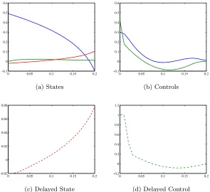
0 2 4 6 8 10 −0.5 0 0.5 1 1.5 2 2.5 3 (a) States
0 2 4 6 8 10 −0.5 0 0.5 1 1.5 2 2.5 3 3.5 (b) Controls
0 2 4 6 8 10 −0.5 0 0.5 1 1.5 2 2.5 3
(c) Delayed States
Figure 3.4: SOCXsolution for IR in Eq. (3.9)
Table 3.1 to describe the closeness of theSOCXapproximation to truth. Figure 3.2 summarizes the numerical results and mesh refinement performance for SOCX, and presents comparable information when the problem is solved using the method of steps. For this problem we solve the method of steps formulated problem on an initial grid of 21 points also to showcase the drastic difference in execution mechanics. Although the method of steps solution yielded a smaller final grid, the computation time is much longer (about 2 times). MOS can be efficient in some cases, but is very slow because of the large systems needed to be solved.
Figure 3.5: Bar graph representation of final time grid for IR in Eq. (3.9)
Table 3.1: Estimated absolute max errors for IR in Eq. (3.9)
State Error Control Error
x1(t) 4.8E-03 u1(t) 5.4E-03
x2(t) 5.1E-03 u2(t) 6.1E-04
x3(t) 5.0E-03 u3(t) 5.3E-03
Table 3.2: Solution comparison for IR in Eq. (3.9)
SOCXSolutions
Gk N Fc Fe ǫ Time
1 21 11 111 7.19E-02 3.20E-02 2 41 8 143 4.57E-03 6.14E-02 3 41 6 1271 8.90E-04 1.80E-01 4 81 4 418 9.92E-05 1.90E-01 5 87 3 371 3.61E-06 1.76E-01 6 173 3 371 1.57E-07 4.91E-01 7 185 3 371 9.54E-08 5.39E-01
Total 185 38 3056 1.67E+00
MOS Solutions
Gk N Fc Fe ǫ Time
1 21 12 150 7.39E-04 1.82E-01 2 41 5 104 3.86E-05 5.64E-01 3 41 5 1049 1.16E-05 1.88E+00 4 48 3 399 7.70E-07 7.97E-01 5 53 3 399 6.44E-08 9.87E-01
Total 53 28 2101 4.42E+00
3.2.2.2 Control Delay Problem
Studies show that optimal control systems with time delays in the state variable are more frequently considered than time delays in the control variable. Time delays in the control occur just as often as they do in the state. However, they are less often studied for the complexity that they introduce into the optimal control system when they depend on future values of the state variable. A minimum energy problem with a delay in the control variable is featured in [7]. The optimal control problem is to minimize the state x(t) using the minimum energy of control u(t). Consider the scalar linear system
˙
x(t) =x(t) +u(t−0.1) +u(t), (3.10a)
with the initial conditionx(0) = 1 andu(s) = 0 fors ∈[−0.1, 0). The optimal control problem is to find the controlu(t), t ∈[0, T], that minimizes the criterion
J = 1 2
Z T
0
u2(t) +x2(t)dt, (3.10b)
The true solution for Eq. (3.10) is plotted in Figure 3.6. Observe that both the state and control are strictly increasing functions. On [0, 0.1] the state is linear as it is impacted by the control delay. The control is being minimized with u(0.25) ≈ 0. The values of the state and the objective function at the final moment T = 0.25 are x(0.25) = 1.173 and J(0.25) = 0.154. SOCXterminated with a solution within a tolerance of 10E-07 in 6 iterations with a final grid of 73 points. The final iteration is plotted in Figure 3.7.
0 0.05 0.1 0.15 0.2 0.25 1
1.05 1.1 1.15 1.2
(a) State
0 0.05 0.1 0.15 0.2 0.25 −0.5
−0.4 −0.3 −0.2 −0.1 0 0.1 0.2
(b) Control
Figure 3.6: MOS solution for the control delay problem in Eq. (3.10)
Graphically the final state and control solutions are comparable to the MOS solutions. However, we see some odd behavior in the control near t = 0.1. This behavior is carried over into the delay control approximation as shown in Figure 3.7c. In Figure 3.8a we zoom in at this node to get a better view of the solution. Neart= 0.1 there are a couple of spikes and dips in the solution. We also plot the first iteration in Figure 3.9 to get a view of the solution on the initial uniform grid of 21 points. Note that the solution results for both state and control are smooth at this iteration. Associated max errors associated with this run are ku(t)−u∗(t)
k=1.42E-02 and kx(t)−x∗(t)
k=4.49E-04.