Microsatellite Genetic Distances With Range Constraints: Analytic Description and Problems of Estimation

Copyright 6 1997 by the Genetics Society of America

Microsatellite Genetic Distances

With Range

Constraints:

Analytic Description and

Problems of Estimation

Marcus

W.

Feldman,*>t

Aviv

Bergman:

David D.

Pollockt

and David

B. Goldstein+-*

*Department of Biological Sciences, Stanford University, Stanford, California 94305, +Interval Research Corporation,

Palo Alto, California 94305 and iDepartment of Zoology, University of Oxford, Oxford OX1 3PS, United Kingdom Manuscript received April 8, 1996

Accepted for publication September 5, 1996

ABSTRACT

Statistical properties of the symmetric stepwise-mutation model for microsatellite evolution are studied under the assumption that the number of repeats is strictly bounded above and below. An exact analytic expression is found for the expected products of the frequencies of alleles separated by k repeats. This permits characterization of the asymptotic behavior of our distances Dl and ( 6 ~ ) ' under range con- straints. Based on this characterization we develop transformations that partially restore linearity when allele size is restricted. We show that the appropriate transformation cannot be applied in the case of varying mutation rates

(0)

and range constraints ( R ) because of statistical difficulties. In the special case of no variation in

p

and R across loci, however, the transformation simplifies to a usable form and results in a distance much more linear with time than distances developed for an infinite range. Although analytically incorrect in the case of variation in

p

and R, the simpler transformation is surprisingly insensitive to variation in these parameters, suggesting that it may have considerable utility in phyloge- netic studies.

M

ICROSATELLITES are a special class of tandemly repeated DNA in which a specific motif of 2-6

bp is repeated up to -100 times (TAUTZ 1993). Micro- satellite loci with

>

-10 repetitions of the basic motif are highly variable in taxa ranging from plants to verte- brates (LAGERCRANTZ et al. 1993). It is common to ob- serve heterozygosities of 0.8 and as many as 20 or more alleles at a locus (BOWCOCK et al. 1994; MACHUGH et al.

1994; DEKA et al. 1995; GOLDSTEIN and CLARK 1995). Microsatellites are also very easily scored using PCR-

based methods and tend to be reliably variable in all populations of a given species. Another important ad- vantage is that microsatellite analyses provide informa- tion about the state of specific loci, facilitating a num- ber of population-genetic inferences.

For these reasons, microsatellites are rapidly replac- ing allozymes and newer markers (e.g., randomly ampli- fied polymorphic DNAs) in studies attempting to esti- mate demographic and evolutionary parameters of natural populations (MACHUGH et al. 1994; ESTOUP et al. 1995; GOLDSTEIN et al. 1995c; SLATKIN 1995a,b). They are also beginning to be used to estimate phyloge- netic relationships among populations and closely re- lated species (BOWCOCK et al. 1994; MACHUGH et al. 1994; DEKA et al. 1995; ESTOUP et al. 1995; GOLDSTEIN

et al. 1995a,b; PEPIN et al. 1995), but success here has been limited both by the availability of variable micro- satellites in multiple species, and by uncertainty as to

Corresponding authw: Marcus W. Feldman, Department of Biological Sciences, Stanford University, Stanford, CA 94305-5020.

E-mail: [email protected]

which genetic distance measure is most appropriate for microsatellites ( GOLDSTEIN et al. 1995a).

The variability of microsatellite loci is due to their exceptionally high mutation rate, which seems to aver- age -0.0001 (WEBER and WONG 1993). This high muta- tion rate also guarantees that isolated populations di- verge rapidly, but an exact description of this process of divergence is elusive since it depends on the precise details of the mutation process. Direct studies of micro- satellite mutation mechanisms, based both on artificial constructs in yeast (HENDERSON and PETES 1992) and analyses of human pedigrees (WEBER and WONG 1993) have shown that most mutations involve the addition or subtraction of a small number of repeat units. This contradicts the assumptions of the infinite alleles muta- tion model, in which all new mutations are to alleles not previously represented in the population. To ac- count for this aspect of the mutation process, a number of authors have recently studied the stepwise mutation model, which was first developed to describe the evolu- tion of the charge state of proteins as inferred from electrophoretic mobility (OHTA and KIMURA 1973).

Using different methods, GOLDSTEIN et al. (1995a) and SLATKIN (1995a) both demonstrated that an unbi- ased estimator of separation time can be obtained by taking the squared differences of all pairs of alleles drawn one from each of the two populations. Subse- quently, GOLDSTEIN et al. (199513) showed that a related distance, given by the squared difference between the means of the two populations, is also linearly related to time. This distance, called (Sp)*, has the further advan- tage of being independent of population size when p o p

ulations are internally at mutation-drift equilibrium. Al- though analytically unbiased, sampling effects may inflate (Sp)' in practice unless sample sizes are relatively large. The linear relationship with time of these step- wise distances is in contrast to traditional distances (e.g.,

Fs7., Nei's distances), which are well known to possess an asymptote under stepwise mutations (NEI and CHAK- RABORTY 1973; CHAKRABORTY and NEI 1977; NEI 1987).

The analytic descriptions in GOLDSTEIN et al. (1995a) and SLATKIN (1995a), however, were highly idealized. Most importantly, both assumed that microsatellite al- leles can have an arbitrarily large number of repeats. Noting that allelic sizes are in fact tightly constrained, GOLDSTEIN et al. (1995a) emphasized that their distance would also asymptote when applied in practice. While lacking a formal model including range constraints, GOLDSTEIN et al. (1995a) presented a heuristic argu- ment suggesting that the value of their stepwise distance at maximal divergence is about (R' - 1)/6, where R is the number of alleles possible. They also provided a very rough estimate of the duration of linearity by calcu- lating how long it would take to reach this value in the unconstrained model.

The exact value of this asymptote and the exact de- tails of the approach of the distance to its maximal value are of critical importance to the evaluation of stepwise distances. For the unconstrained model, both SLATKIN (1995a) and GOLDSTEIN et al. (1995a) demon- strated that nonstepwise distances are more accurate for closely related taxa, but that stepwise distances become superior beyond some critical level of divergence. Intu- itively, the stepwise distances become superior after the nonstepwise distances have lost linearity and no longer accurately reflect separation times. With range con- straints, however, stepwise distances also asymptote and should work better only within a certain window of sepa- ration times. The lower boundary of this window is re- lated to the time at which nonstepwise distances asymp- tote, and the upper boundary is related to the time at which the stepwise distance reaches its asymptote of ( R 2 - 1)/6. It is also important to appreciate that this window in which stepwise distances are superior will only exist if R is sufficiently large. GOLDSTEIN et al. (1995b) used polymorphisms in three primate species to investigate experimentally whether the level of diver- gence among closely related primates falls within this window. They showed that (tip)' allows the three possi- ble rooted trees relating humans, chimps and gorillas to be distinguished, while Nei's distances, for example, do not.

For a more rigorous assessment of the reliability of different distances under range constraints, and to de- velop statistical corrections to recover linearity, it is nec- essary to have an analytic description of the dynamics of genetic distances under range constraints. Here we introduce an analytic framework that allows an exact description of the expected dynamics of loci undergo-

ing stepwise mutations on a restricted set of R alleles. GARZA et al. (1995) recently proposed a model of micro- satellite evolution that incorporates bias in the muta- tion process in the form of a "restoring force" such that small alleles tend to mutate upward and large alleles downward. In the present study, we incorporate explicit range constraints for the following reasons. First, maxi- mal and minimal allele size would seem much easier to estimate than a parameter governing the degree of asymmetry in the mutation. This difference becomes especially important in connection with attempts to im- prove genetic distances by applying corrections based on parameters that must be estimated. A second motiva- tion is that an explicit upper ceiling seems to be a closer representation of the known behavior of certain micro- satellites (e.g., trinucleotides) in which the mutation process is more symmetric and the rate moderate for small alleles, while for larger ones the rate is extremely high and biased upward. If we assume that the large alleles are severely disadvantageous, a fixed range be- comes an appropriate representation. For simplicity, we consider only the strict stepwise mutation model.

Dealing with an infinite number of allele sizes, previ- ous models (OHTA and KIMURA 1973; MORAN 1975) have described the evolution of the expected products of allele frequencies separated by k units, given by

ck

=

Ej

v,vi+k, where v , and v i + k are the frequencies of

alleles with i and i

+

k repeats. In the case of finite R , however, it is straightforward to show that a closed form recursion for the

ck

cannot be obtained independent of the underlying allele frequencies. Studying variation within a single population NAUTA and WEISSING (1996) approximated the frequencies of boundary terms in each of the C,. Here we instead describe directly the evolution of the matrix of expected products of allele frequencies. The traditional C k can be obtained from such a matrix by summing diagonal rows. This analysis confirms the numerical results obtained by NAUTA and WEISSING (1996) and allows us to obtain analytic expres- sions for the expectations of measures of variation within a population. More relevant to our purposes here, we also introduce the interpopulational sum

C f , which is the sum of products of allele frequencies drawn one each from two isolated populations. We show how this is related to our distances (tip)' and ASD, a distance we introduced earlier (GOLDSTEIN et

Microsatellite Range Constraints 209

single population (GOLDSTEIN et al. 1995a). In practice,

Do may be calculated as twice the within-population vari- ance in repeat sizes. We also show that the rate of con- vergence to this maximum is given by (1 - 2P

+

2P

cos 7r/R)‘, where /? is the stepwise per locus mutation rate. On the basis of these results, we outline the form that any correction must take to provide a statistically unbiased estimate of separation times. As we shall see, the required form ensures that such corrections will not be applicable in the general case in which

P

and R

vary across loci. Nevertheless, in the special case of sets of loci with the same

P

and R, a simple analytic correc- tion can lead to less biased estimation of separation times without the statistical complications that arise in the general case. We use computer simulations to assess the reliability of the correction in this special case and compare the performance of the new estimator to ex- isting estimators like (Sp)‘. We also test the sensitivity of the simplified distance to variation in and R and find that it continues to behave well, despite being for- mally inappropriate in this case.

METHODS AND RESULTS

The following analysis is based on that of MOW (1975) who derived a number of important results for the stepwise mutation model in which there is no con- straint on the number of repeats occurring at a locus. Here we specify a range R of repeat scores, and for convenience these are represented as 1 , 2 ,

. . .

,

R. Thus,

R is the possible number of alleles. Symmetric one-step mutation is postulated so that for any allele i the rate of mutation to each of i - 1 and i

+

1 is

P.

At time t the number of (haploid) genes carrying

i

repeats is

ni( t ) with

C i

ni( t ) = N, the population size. After muta- tion, the population frequency of allele i is

with

? r l ( t ) = (1 -

Multinomial sampling then takes place to produce the next generation of alleles. Writing E,, as the expecta- tion operator in generation t given the frequencies at time t - 1, we have for i = 1, 2,

.

. .

, R ,

E t - l [ n i ( t ) n j ( t ) l

= N ( N - l)7rZ(t - 1)7rl(t - l ) , i f j (2a)

Et-l[n7(t)] = N(N- l ) ~ : ( t - 1)

+

Nr,(t - 1). (2b)

In our earlier studies of microsatellite evolution, two functions were used to study the evolution of allele frequencies within and between populations. These were Do, the average squared difference in repeat num- bers for two alleles drawn from the same population, and Dl, the same average when the alleles are drawn one each from different populations. (Note: We have used the average square distance symbols ASD and Dl interchangeably in our earlier papers. Here we shall use Dl for brevity.) The time-dependent behavior of these functions when there is no restriction on the range of repeat numbers can be studied directly (GOLDSTEIN et al. 1995a). In particular, the difference Dl - Do, denoted (Sp)‘, provides a useful distance that is linear in the time since the separation of the two populations and removes the effect of population size

(GOLDSTEIN et al. 199513; ZHIVOTOVSKY and FELDMAN 1995).

In the absence of range restriction, MORAN (1975) analyzed the model in terms of the moments of the quantities

where we may write

Do

= 2 i2Cj. (4)

2

A similar sum of products with the alleles chosen from each of two populations gives rise to Dl:

Dl

=

2

i‘CT (5)

with

C $ ( t ) = C l k ( t )

and the superscripts to refer to the two populations ( a )

and ( b ) .

The quantities C, and CT appear to be more difficult to analyze directly in the case of restricted range and we have chosen an approach that uses each of the sum- mands in ( 3 ) and (6).

Analysis: Denote by B the R X R matrix with ele- ments Bll = Bm = 1 -

P;

BIj = 1 - 2P for i

+

1, R;

= B1-,,, =

P.

This tridiagonal matrix represents the one-step mutation process with forward and back- ward rates each

p.

Denote by v, the (row) vector of R

allele frequencies n1 ( t )

/

N, n, ( t )

/

N. * nR( t ) / N at time t . Then we may rewrite the relations (Equation 2) using the symmetry of B as

&I (v?vt)

where A, is the R X R matrix with 1 in the

(i,

i ) position and 0 elsewhere, ei is the 1 X Rvector with 1 in position

i

and 0 elsewhere, and the superscript T represents the transpose. Relation 7 reports the expectation after a generation of multinomial sampling conditioned on generation t

-

1. Upon iteration we obtain the expecta- tion given the initial frequencies

+

i

1 - - B~VOT~OB'. (8)

k)

It is clear that BfvTconverges to the uniform probabil- ity vector (l/R, 1/R,

.

.

.

,

l/R)T. The rate of conver- gence is the second largest eigenvalue of B, namely

(BARNETT 1990,

p.

350; the largest is obviously X. = 1).

This enables us to write

= I [ I - (1 -k)B'] = Z , ₍₁₁₎

- 1

RN

say, where I is the identity matrix.

The entries of the matrix Z give us the equilibrium expectations of products of frequencies (nJN) (nj/N)

(i,

j = 1 , 2 ,

. . . ,

R). Equilibrium values of C,

(as

defined in Equation 3 above) are obtained by summing the appropriate diagonal entries of Z. In principle, we may then compute Do as in (4).

First, let us examine the series in (10). The entries of the powers B'J are polynomials in @. Only the diago- nal and the first super- and subdiagonals have linear terms in @. The (1, 1) and ( R , R) elements of B'J are

(1 - Zpj), while the (i, i) elements ( i f 1, R ) are 1 -

4@j, neglecting terms O ( @ * ) . Upon summation, how- ever, these terms in @' actually turn out to be O(@N)'. If @N

<

1, then to order

(PN)',

C,, = 1 - 4 @ ( N - 1 ) ( 1 -

i).

(13)

In the same way, we may compute Cl = C 1 ,

= 2 @ ( N - 1 ) ( 1 -

;)

,

where again terms O(@N)' are neglected. To this order of accuracy, we may write

&(Do) = EO(C1)

+

&(C-l) (15)

= 4 @ ( N - 1 ) ( 1 -

;)

.

Remark: As R -+ UJ in (15) we obtain the result of GOLDSTEIN et al. (1995) derived from MOW (1975).

Note also that for large N and NP small,

C,

in (13)

approximates (1

+

8Nfl)"", the result obtained by KIMURA and OHTA (1973) and MORAN (1975). It is im- portant to stress that the approximation made by ne- glecting (NP)' and higher powers may not be good, especially when R is small. It appears that in computing

Do, terms of the form

( P N ) k

vanish, leaving only terms of the form ck(PWk/R, where ck are constants. For PN

large and

R

small, these may be important.

As

an exam- ple, retaining the terms in

(PN)'

and

(PN)'

gives the extension of (14):

&(Do)

= 4 P ( N - 1) 1

( ;)

- - -

-

(4N' - 7 N

+

3)

4 :

+

P 3 ( N - 1)'(2N - 1 )

+

O(@W4.

(16)

We conjecture that all higher powers of

( P N )

will also occur only with a divisor of R. Since (NP) is typically quite large (GOLDSTEIN and CLARK 1995; GOLDSTEIN et

al. 1995b), it will usually be necessary to determine &Do by numerical evaluation of the matrix Z in ( 1 1).

To study the problem of differentiation between p o p ulations, suppose that a population has reached the equilibrium defined by

( l o ) ,

that two populations are formed from this progenitor population and that ini- tially each has the same statistical configuration as the ancestral group. Subsequently, the evolution of the two groups, labeled a and b, occurs independently. Write .vL and bvt for the (row) vectors of allelic frequencies in the two groups. Then, as before, we have

16

E,-l(,vF)

= B,v;cI,

~ 5 - ~ ( p ; )

= Bbv;II,

and, after sampling in the two populations,

&-1[,v:'

PJ

= BRLI Y-IB,

Microsatellite Range Constraints 21 1

&[avT

bvtl = B'HavOT POIB'.

(17)

Here, E[,V:

p o l

represents the state of the initial popu- lation given by Z in ( 1 1 ) . Hence

Now each summand B2(t+J' converges to the matrix B = llBoil with Bii = 1 / R at the rate (1 - 2 p

+

2 p cos r/

R)', which is the leading nonunit eigenvalue of B2. We conclude that for each entry of the matrix on the left of ( W ,

lim

{&[yT

b ~ t ] } y = l/@, i , j = 1, 2 .

-

* R. (19) We may now compute the equilibrium value of

Po

&(Dl ),

R

&(Dl) = 2

c

E&(CT)

i= 1 R R-i

= 2

2

1 / R 2

i = l j = 1

R

= 2 E(R - i ) / R 2

i= 1

= ( R 2 - 1 ) / 6 . ( 2 0 )

This is the value postulated originally by GOLDSTEIN et

al. (1995a) and used by NAUTA and WEISSING (1996); it can be obtained directly by noting that the allele frequencies within a population approach a uniform distribution.

In populations a and b, denote the average repeat scores at time t by ra( t ) =

C

i,v: and r b ( t ) =

C.

ipi.

GOLDSTEIN et al. (1995b) defined the distance between

populations a a n d bby (Spt)' = ( r a ( t )

-

r b ( t ) ) 2 at time

t . It is easy to see (GOLDSTEIN et al. 1995b)

E t - l ( S ~ t ) ~ = Et-1 (Q(O) - Va(t)

-

V,(t), where V J t ) and &(t) are the variances in populations

a and b at time t, and therefore & ( S P , ) ~ approaches the limit

ii(Sp)2 = ( R 2

-

1)

6

-

EODO

as t + m. For PNsmall,

E&

may be estimated as in (15); otherwise, it must be calculated numerically. Recall that without restriction on the range of repeat scores, &(Sp,)' grew as 4p7, where

r

is the time since popula- tions a and b split from a common ancestral population. Under the assumption that the ancestral population had reached equilibrium (Le., &(Do) was at its equilib- rium value), then &(bp)' changes at the same rate as

&(Dl),

namely (1

-

20

+

2 p cos T / R ) ~ . When t is small and R is large, therefore, ( 6 ~ ) ~ will grow approxi- mately as in the unconstrained case.

Statistical issues: We showed above that the rate of convergence of E ( D l ) and E ( S P ) ~ are governed by the second largest eigenvalue of the matrix B2, namely (1

-

2 p

+

2 p cos 17/R)2. Here we focus on ( S P ) ~ , since that seems to be the preferred distance, and write

E(Sp)T(t)

= M(Ri) [l - (1 - 2 p ,

+

2pi COS T / R ~ ) ' ~ ] , ( 2 3 )

where the subscript

i

represents a mutation rate and a range specific to locus i , and

M(R,,)

is the maximum value of the distance. For

p

small, this equation can be approximated as

E(Sp)T(t)

= M ( R i ) { l - exp[-(4Pi

-

4pi cos r / R i ) t ] } . ( 2 4 )

The asymptotic behavior of the stepwise distance guar- antees that after sufficient time has passed, it will pro- vide a biased estimate of separation times. In such cases, it is sometimes useful to find a correction that results in a linear distance, although this often entails too high a price in terms of the variance of the distance

( GOLDSTEIN and POLLOCK 1994). To obtain a distance whose expectation is linear with time in the general case where R and

p

vary across loci, it is necessary to take the product of the differences between the ob- served and maximal distances across loci. For conve- nience we will represent each of these differences as a fraction,

P,,

of maximal distance. That is,

P,

=

( M ( R . )

- E(D1,i))/M(&.). To obtain afunction linearwith time using all of the loci, we take the product across loci of the P,:

=

n

exp[-(4pi -

4pi

cos x / R , ) t ] . ( 2 6 )

Taking the logarithm of the products of the

Pi

results in a distance that is linear with time.

1

log

n

P

i

=

-x

(4pi

-

4pi COS r / R i ) t ( 2 7 )

= Clt, ( 2 8 )

say, where C, =

- X i

(4pi - 4pi cos

r/R,)

is a constant given by the sets of

p i

and R,. When mutation rates and range constraints are known, time can be obtained directly using the reciprocal of Cl

.

When the mutation rates are not known, a linear function can be obtained as long as the R, are known so that

Pi

can be obtained. Since Cl is negative, the distance in this case would be obtained as -log

[n,

Pi].

of this distance are highly undesirable. The basic prob- lem is that

Pi

must be calculated for each locus sepa- rately. Since stepwise distances have a high variance (GOLDSTEIN et al. 1995a; ZHIVOTOVSKY and FELDMAN

1995), many of the Pi will be negative, even when the expectation of (Sp)' is well below M ( R , ) . When one or more of the Pi is negative, the argument of the loga- rithm is negative and the distance cannot be calculated. Consequently, all loci for which Pi

<

0 must be either discarded from the analysis or set to an arbitrary value. We used computer simulations (described below) to evaluate the behavior of -log

[ni

Pi]

as a distance.

As

might be expected, discarding atypically large values results in a substantial bias, causing -log

[ni

Pi] to asymptote even earlier than (Sp)' (data not shown). It is conceivable that some method that truncates large distances at an arbitrary value would work better, but we are not optimistic that the behavior can be substantially improved.

For completeness it should be noted that even in the unlikely case that M(R,.) is sufficiently greater than the expected distance to ensure that no domain errors oc- cur, the distance still would not be likely to perform well. Since the Pi vary stochastically, and the function required to restore linearity is highly nonlinear, the correction has a substantial bias. To determine how the linearized distance -log

[ni

Pi] is influenced by variation in the Pi let g(Pl, P2,

. . .

,

PL) = log

[ni

Pi].

Then, the expectation of g(Pl, P2,

. . .

,

P 2 ) can be esti- mated using the delta method (see for example RICE

1995, p. 149):

E[g(Pl, P2, * * f 3 PL)1 = g[W1),

W'),

. .

.,

W L ) I

1 d2

2 , d e

+-x.Var (Pi) - - - g [ ~ W 1 ) , W ' 2 ) ,

. . .

, W L ) I .

(29)

[To obtain (29), covariances have been neglected.

ZHIVOTOVSKY and FELDMAN (1996) showed that these covariances are indeed negligible when the recombi- nation between all pairs of genes is large relative to

1/N. Our simulations indicate that these covariances are much less than the variances of Pi.] Because

d ' g / d e = -1/[E(Pi)]' is negative, the expectation of

the linearized distance is always a smaller negative num- ber than g [ E ( P l ) , E ( P 2 ) ,

. .

.

,

E(PL)]. That is, the dis- tance has the form - ( Clt - k ) and this is larger than it should be (recall Cl is negative). Furthermore, the magnitude of the error is proportional to the variance of P,, which is known to be very large (ZHIVOTOVSKY

and FELDMAN 1995). Although this bias might be cor- rectable, statistically it seems hardly worthwhile to make the effort.

In summary, there are two difficulties in employing this correction to recover linearity. (1) Some of the Pi

will be negative, causing a log domain error that cannot be eliminated without introducing a substantial bias, and (2) taking products results in very biased estimates

even when a domain error does not occur, the bias being proportional to the variance of the distance at a single locus. We are not optimistic about the prospect of overcoming these problems with any analytic estimator.

A solution to these problems is straightforward, how- ever, in the special case in which

Pi

= p and R, = Rfor all i: that is, mutation rates and range constraints do not vary across loci. In this case we may work with the arithmetic average of the distances across loci as follows.

Ex

(6CL)T

=EM(R)(l-exp[-(4P-4Pcos7r/R)t]) (30)

= LM(R)(l -exp[-(4P--4Pcos7r/R)t]), (31)

where L is the number of loci. Then a linear distance based on an arithmetic average is obtained as,

That is, the proposed distance, DL, is constructed by summing (Sp)' across loci, dividing by L times the pre- dicted maximum (Equation 22) and, subtracting this from 1, taking logarithms and dividing by - C2. The improvement can readily be seen with a procedure simi- lar to that used in (29). In this case, the arithmetic averaging results in a bias that falls with the square of the number of loci. After discounting for the difference between Cl and

C2

in (28) and (32), the bias of the summed distance is 1/L times that of the product dis- tance. More importantly, combining observed distances arithmetically greatly reduces the chance of a log do- main error. Finally, since the variance of CDl,i as a pro- portion of LM decreases with the number of loci, the probability of a domain error goes down as the number of loci increases. This suggests that for a sufficiently large number of loci, all with the same mutation rate and range constraint, the log correction shown above might have practical use.

Computer evaluation: The properties of DL as a ge- netic distance were tested using computer simulations similar to those described in GOLDSTEIN et al. (1995a). A single population is brought to equilibrium under step wise mutation and drift and an identical copy is then made. The independent evolution of these two popula- tions is simulated, and at set intervals of time, distances are calculated. Figure 1 shows the average behaviors of

Microsatellite Range Constraints 213

40 Loci

40 Loci

'

6ooa

3

8

400C

."

B

Y

200c

C

Generations

EO Loci

Generations

FIGURE 1.-Simulation results of two populations starting

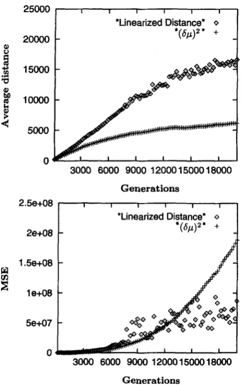
at the same equilibrium state. Each population has 100 indi- viduals with either 40 or 80 loci each. The mutation rate per locus per generation was 0.01. Results reported here are averages over 500 replicates with different initial conditions. (Top) ( 6 ~ ) ' and linearized distance (DL) computed as aver- ages over 40 loci (per individual), all having the same range constraint ( R = 20). (6p)' has been divided by 4p to make it comparable to DL. The x a x i s is the number of generations, and the y axis is the estimated time calculated from the o b served distance. [Upper curve DL, lower curve (Sp)'.] (Bot- tom) Same as A but with the averages over 80 loci (per individ- ual) of (Sp)' and DL.

divergence, LM, resulting in a log domain error. As noted above, we expect that for given t, the chance of satiswng the inequality

LM

- Z(Sp)S

<

O (thus causing a log domain error) will decrease with the number of loci, thereby extending the time over which DL will re- main linear with t . The simulation with 80 loci confirms this expectation. In this case DL is approximately linear until generation 10,000 or so. As would be expected, the linearity of (Sp)' is not affected by the number of loci; therefore DL, unlike (Sp)', has the interesting property that its useful temporal range can be extended by in- creasing the number of loci studied.

To compare the overall reliability of the two dis- tances, we use the mean squared error (MSE)

.

Suppose that the values of either (Sp)' or DL are observations on the following process: A ( t ) = t

+

b

+

E , where A ( t ) is the estimated time using either (tip)' or DL as the time estimator, t is the true time of separation, b is a

1.2e+OB .

1.0e+08

.

2.0.2

+

07 .

0 2000 4000 6000 8000 10000 12000 14000

Generations

BO Loci

1.4e+O8 '

t B

/

1.2e+OB.

1.Oe + MI .

w 8.0e+07

VI

E

6.Oe+07

4.0e + 07

1

/-&

2.0e+07

0 .

0 2000 4000 6000 BOO0 10000 12000 14000

Generations

FIGURE 2.-Mean square errors. (A) The mean square er-

ror (MSE) (see text) of (Sp)' and DL as functions of separa-

tion time between two populations of individuals with 40 loci each (averaged over all 40 loci). [Upper curve (6p)', lower curve DL.] (B) Same as A but with two populations of individ- uals with 80 loci each (averaged over all 80 loci).

constant, or systematic, error, often called the bias, and E is the random component of the error. Here E is a random variable with E [ € ] = 0 and Var ( E ) = a'. An overall measure of the size of the error is the MSE,

which is defined as

MSE = E [ ( A ( t ) - t ) ' ] .

MSE can be decomposed into contributions from the bias and the variance as follows:

MSE =

b2

+

a'.

The values of (Sp)

'

and DL are computed as the average over all loci, either 40 or 80, and over all

500

replicates of the simulation. The values of MSE and

a'

are mea- sured over the 500 replicates. Figure 2A demonstrates that, due to the asymptotic behavior of (Sp)', its MSE

very quickly becomes substantially larger than that of DL. Figure 2B shows that this difference increases with the number of loci, as expected.

Another way to assess the expected performance of these distances in phylogeny reconstruction uses the accuracy index introduced by TAJIMA and TAKEZAKI

may perform better, especially with a large number of loci. Since the slope of (Sp)' is not sensitive to the number of loci, and the point at which the linearity of

DL is lost increases with the number of loci, it seems clear that for a sufficiently large number of loci and sufficiently large t , DI, will have a higher accuracy than

( 6 ~ ) ' . These theoretical considerations suggest that DL

has potential as a distance for microsatellite loci. The major difficulty in its implementation is finding a large number of microsatellite loci with sufficiently similar mutation rates and range constraints. Fortunately, it

would appear that DL is not highly sensitive to moderate variation in

p

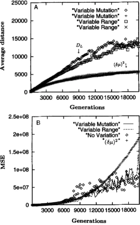
and R.

To assess the sensitivity of DL to rate variation, we compared simulations with constant and variable ranges and mutation rates. We considered 30 loci in which the mutation rate was either fixed at 0.045 or chosen randomly from the interval 0.015-0.075 for an average of 0.045. Similarly, the range R was either fixed at 60 or chosen randomly from an interval of 20-100 for an average of 60. Figure 3 presents the results from the simulation with constant

R

and

p,

while Figure 4

show the simulations with variable R and

0.

The most striking aspect of these results is that even though the transformation is analytically incorrect when R and

p

vary, applying this transformation when either

R

or ,B

vary over a factor of 5 (Figure 4) results in behavior almost identical to that when the transformation is ap- plied to a set of loci with fixed values that are the aver- ages of the varying values (Figure 3). That is, under variation in either R or

0,

DI. remains much more linear than (6p)' and in fact is nearly as linear as it is in the case of no variation among loci. Furthermore, the MSE of the transformed distances remains well below that of

(by)' for the bulk of the evolution, and is even generally below that of 0,. applied to the case of no variation (Figure 4B). These results suggest that DL, despite be- ing an inappropriate transformation analytically, never- theless behaves very well in the case of variation in

p

and

R.

Careful inspection of Figure 4B also reveals that the MSE of DL in the case of fivefold variation in R is some- what lower than in the case of fivefold variation in

/?.

This suggests that DL is less sensitive to variation in R

than variation in

P,

as might be predicted based on the expectation shown in (31). Notice that the only place where variation in R will affect linearity is in the term cos n / R inside the exponential. This is the only im- portant term because the leading LM(R) averages, and the term against the exponential will only contribute an additive term upon log transformation. Because cos

n / R in the exponential is asymptotic in R, as long as all loci have reasonably high values of R (say above 25 or so), variation in R is expected to have a relatively small impact. Variation in

p

is expected to be more important because it is linear inside the exponential term. Thus, in applying DL it would seem that clumping

25000

J I I I I I I 1

20000

I

"Linearized Distance" Q

-

'(Sp)2" +

1 0000

5000

0

3000 6000 9000 12000 15000 18000

Generations

2.58+08

I I I I I I

"Linearized Distance" o

2e+08

1

3000

6000

9OOO

1200015000 18OOO

Generations

FIGURE 3."Constant parameter simulations. Conditions

are the same as above except that the mutation rate is 0.045, R

is 60, and the population size is 60. Top: the average distances among 150 replications; bottom: the MSE for each of the two distances.

loci into sets with similar mutation rates will be more critical than clumping them on the basis of R.

DISCUSSION

The tremendous variability of microsatellite loci has established them as the preferred markers for most intra- specific applications. Their use in interspecific phylog- eny reconstruction, however, has been much less success- ful. One reason for this seems to be that at least some microsatellites degrade quickly, causing their mutation rates and other parameters to differ greatly from taxon to taxon (ELLEGREN et al. 1995; RUBINSZTEIN et al. 1995; GOLDSTEIN et al. unpublished data). As a result, distances at these loci do not appear well correlated with time for more divergent taxa. Another difficulty is that even when microsatellites persist over suf€iciently long intervals, they

Microsatellite Range Constraints 215

"Variable Mutation'

"Variable Range'

a 20000

2.5e

2e

-

3000 6000 9000 12000 15000 18000

+08

+08

1.56+08

w

E

le+08

v3

5e+07

0

Generations

I I I I I I

B "Variable Mutation" - 'Variable Range"

-

_{"No Variation" 0}

_:-

-

3000 6000 9000 12000 15000 18000

Generations

FIGURE 4.-Variable parameter simulations. Conditions are

the same as in Figure 3 except that either the mutation rate is randomly drawn from the interval (0.015, 0.075) (average of 0.045 as used above) or the range constraint is randomly drawn from the interval (20, 100) (average of 60 as for Figure 3). (A) The average distances among 150 replications. The two upper curves are the transformed distances (applied in the case of variable R or variable p ) and the two lower curves are

(SF)'.

(B) The MSE for the linearized distance applied to all three cases (no variation, variation in R, and variation in p). The MSE for

(SF)'

is the same for all cases, so only one curve is shown.

have been well established empirically (BECKMANN and

WEBER 1992; BOWCOCK et al. 1994), mean that microsat- ellites will eventually lose their phylogenetic information (GOLDSTEIN et al. 1995a,b). Here we have outlined an analytic method for characterizing the effect of a specific constraint on maximal allele size. Based on this analytic characterization, we have developed new distances that recover the linear relation with time even when ranges are constrained.

Our analysis incorporates what seems to us the sim- plest mutation process with fixed range constraints. For all i allelic states for 1

<

i

<

R symmetric stepwise mutations occur at a rate

p

in each direction. For the

boundary states I and R , mutation only increases or decreases size, respectively, again at a rate of

p.

In real- ity, it is clear that the mutation process has a much more complicated dependence on allele size (RICHARDS

and SUTHERLAND 1994; GOLDSTEIN and CLARK 1995). Unfortunately, the exact details of the mutation process are not sufficiently well understood to allow an accurate representation. Furthermore, they are likely to mry from one type of microsatellite to another. As such details become available it will be worthwhile to develop more complicated models. In theory, the analytical ap- proach employed here allows arbitrary assumptions about the mutation process since an explicit transition matrix is used. In practice, however, it may be that all but the simplest matrices will resist direct analysis. It seems reasonable to assume, however, that the primary conclusions obtained here reflect the existence of range constraints and are likely to apply when other assumptions are made about the exact details of the process imposing the limits on size. This conjecture is supported by the qualitative similarity of our results to those of GARZA et al. (1995) who used different analytic techniques and assumed a very different mutation pro- cess.

One important general point to emerge from this study is that it is probably not possible to develop a formally accurate analytic distance for microsatellite loci in the general case in which mutation rates and range constraints vary across loci. This follows from the form of the distance under range constraints, which necessitates multiplying distances across loci before log- arithms are taken. Because of the high variance of the underlying distance, this process invariably results in log domain errors and is therefore essentially useless. On the other hand, we have shown that if a large set of loci with sufficiently similar mutation rates and range constraints can be identified, a simple analytic correc- tion can provide a distance that is much less biased than existing distances. An interesting and unusual property of the new distance is that its linearity increases with the number of loci. Most importantly, we have used computer simulations to show that even though it is formally insufficient to recover linearity in the case of variation among loci, the simple correction i s not strongly sensitive to such variation. If loci can be clus- tered at least to within a factor of 5 or so, Dr. can be expected to substantially improve linearity.

to use the analytic expectations developed here to com- pare the behavior of stepwise and nonstepwise dis- tances. In particular, it is important to delimit the boundaries of the window of time within which stepwise distances outperform nonstepwise distances (GOLD- STEIN et al. 1995a,b). These considerations suggest that variation at certain microsatellite loci might not be use- ful for some phylogenetic problems. Just as one would not use sequence variation in histones or other slowly evolving proteins to assess relationships among closely related species, one must choose microsatellite appro- priate to the phylogenetic problem under study. For example, in studying relationships among more diver- gent taxa, it is necessary to choose microsatellites that (1) have not degraded in either taxon, (2) have suffi- ciently large ranges, and (3) have a sufficiently small mutation rate. It is well known that these parameters vary among types of microsatellite loci (WEBER and WONG 1993). Therefore, it is little wonder that the a p plication of microsatellites chosen strictly on the basis of polymorphism in a focal species has been of relatively little use in recovering interspecific relationships. The challenge now is to develop the machinery necessary to estimate the parameters of microsatellite loci. Once these parameters are estimated, models like the one described here can be used to partition microsatellites into categories appropriate for different kinds of phylo- genetic problems. Finally, the statistical properties of the distance to be used must be considered to deter- mine the minimum number of loci required for a speci- fied degree of accuracy. In general, we expect that the requisite number will be somewhat larger than is cus- tomary at present. While the exact numbers will depend on the phylogenetic problem at hand and on the exact parameter values estimated, we doubt that fewer than

-15-20 microsatellites will ever provide very reliable estimates of interspecific relationships. Furthermore, we expect that some phylogenetic problems will require characterization of a great many more loci. Fortunately, eukaryotic genomes seem to harbor sufficient numbers of microsatellites that reliable information should be obtainable if one is willing to invest the effort.

The authors thank Drs. NAUTA and WEISSING for providing an advance copy of their manuscript. This research supported in part by National Institutes of Health (NIH) grant GM-28428 to M.W.F., and an NIH National Service award to D.B.G.

LITERATURE CITED

BARNETT, S., 1990 Matrices: Methods andA@lications. Oxford Univer-

BOWCOCK, A. M., A. RUIZ LINARES, J. TOMFOHRDE, E. MINCH, J. R. sity Press, Oxford.

KIDD et al., 1994 High resolution of human evolutionary trees with polymorphic microsatellites. Nature 368: 445-457. CHAKRABORTY, R., and M. NEI, 1977 Bottleneck effects on average

heterozygosity and genetic distance with the stepwise mutation model. Evolution 31: 347-356.

DEJSA, R , L. JIN, M. D. SHRIVER, L. M. Yu, S. DECROO et al., 1995 Popula-

tion genetics of dinucleotide (dCdA)Fn(dGdT)n polymorphisms in world populations. Am. J. Hum. Genet. 56: 461-474.

ESTOUP,A., L. GARNERY,M., SOLIGNACandJ. CORNUET, 1995 Microsat- ellite variation in honey bee (Apis MeZlz@ra L . ) populations: hier- archical genetic structure and test of the infinite allele a n d s t e p wise mutation models. Genetics 140: 679-695.

G m , J. C., M. SLATKIN and N. B. FREIMER, 1995 Microsatellite al- lele frequencies in humans and chimpanzees, with implications for constraints on allele size. Mol. Biol. Evol. 12: 594-603. GOLDSTEIN, D. B., and A. G. CLARK, 1995 Microsatellite variation in

Acids Res. 23: 3882-3886.

North American populations of Drosophila melanogmter. Nucleic

GOLDSTEIN, D. B., and D. D. POLLOCK, 1994 Least squares estima- tion of molecular distance-noise abatement in phylogenetic reconstruction. Theor. Popul. Biol. 45: 219-226.

GOLDSTEIN, D. B., A. RUIZ LINARES, L. L. CAVALLI-SFORZA and M. W.

FELDMAN, 1995a An evaluation of genetic distances for use with microsatellite loci. Genetics 1 3 9 463-471.

GOLDSTEIN, D. B., A. RUIZ LINARES, L. L. CAVALLI-SFORZA and M. W. FELDMAN, 1995b Genetic absolute dating based on microsatel- lites and modern human origins. Proc. Natl. Acad. Sci. USA 92:

GOLDSTEIN, D. B., L. A. ZHNOTOVSKY, K. NAYAR, A. RUIZ LINARES, L. L. CAVALLI-SFORZA et al., 1995c Statistical properties of the variation at linked microsatellite loci: implications for the history of human Y chromosomes. Mol. Biol. Evol. (in press). HENDERSON, S., and T. PETES, 1992 Instability of simple sequence

DNA in Sacharomyces cerevisiae. Mol. Cell Biol. 12: 2749-2757. LAGERCRANTZ, U., H. ELLEGREN and L. ANDERSON, 1993 The abun-

dance of various polymorphic microsatellite motifs differs between plants and vertebrates. Nucleic Acids Res. 21(5): 11 11 -1 115. MACHUGH, D. E., R. T. Lonus, D. G. BRADLY, P. M. SHARP and P. CUN-

N I N G ~ , 1994 Microsatellite DNA variation within and among European cattle breeds. Proc. Roy. SOC. Lond. B 256 25-31. MORAN, P., 1975 Wandering distributions and the electorphoretic

profile. Theor. Pop. Biol. 8: 318-330.

NAUATA, M. J., and F. J. WEISSING, 1996 Constraints on allele size at microsatellite loci: implications for genetic differentiation. Ge- netics 1 4 3 1021-1032.

NEI, M., 1987 Molecular Evolutions? Genetics. Columbia University Press, New York.

NEI, M., and R. CHAKRABORTY, 1973 Genetic distance and electro- phoretic identity of proteins between taxa. J. Mol. Evol. 2: 323-

328.

OHTA, T., and K. KIMURA, 1973 A model of mutation appropriate to estimate the number of electrophoretically detectable alleles in a genetic population. Genet. Res. 22: 201-204.

PEPIN, L., Y. AMIGUES, A. LEINGLE, J. L. BERTHIER, A. BENSAID et al.,

1995 Sequence conservation of microsatellites between Bos tuu-

w (cattle) and C a p a hircus (goat) and related species. Heredity POLLOCK, D. D., A. BERGMAN, M. W. FELDMAN and D. B. GOLDSTEIN,

1996 An improved distance estimator for microsatellites with range constraints. Manuscript.

RICE, J. A,, 1995 Mathematical Statistics and Data Analysis, Ed. 2. Dux- bury Press, Belmont, CA.

SLATKIN, M., 1995a A measure of population subdivision based on microsatellite allele frequencies. Genetics 139: 457-462. SLATKIN, M., 1995b Hitchhiking and associative overdominance at

a microsatellite locus. Mol. Biol. Evol. 12: 473-480.

TAJIMA, F., and N. TAKEZAKI, 1994 Estimation of evolutionary dis- tance for reconstructing molecular phylogenetic trees. Mol. Biol.

TAUTZ, D., 1993 Note on the definition and nomenclature of tan- demly repetitive DNA sequences, pp. 21-28 in DNA Fzngnpnnt-

ing; State of the Science, edited by S. D. J. PENA, J. T. EPLEN and WEBER, J. L., and C. WONG, 1993 Mutation of human short tandem

A. J. JEFFREYS. Birkhauser Verlag, Basel.

ZHIVOTOVSKY, L. A,, and M. W. FELDMAN, 1995 Microsatellite

van-

repeats. Hum. Mol. Genet. 2: 1123-1128.

ability and genetic distances. Proc. Natl. Acad. Sci. USA 9 2 6723-6727.

7 4 53-61.

E d . 11: 278-286.

11549-11552.