ABSTRACT
KUMAR, VIKAS. Effect of Shape and Density on Electrical Conductivity of Non-Stochastic Lattice Structures. (Under the direction of Dr. Denis R. Cormier.)
Non-stochastic lattice structures are 3-dimensional arrays of unit cells whose geometric properties can be engineered to tailor the structural, thermal, or electrical properties. In this research, electrical conductivity of five different lattice cell geometries has been calculated. The geometries examined include regular hexahedrons, octahedrons, truncated octahedrons, rhombic dodecahedrons, and hexagonal lattices. The relationship between ligament length, ligament radius, relative density and electrical conductivity has been analytically derived and compared for the different cell geometries. The analysis indicates that electrical conductivity is dependent on the shape of the cell; it increases with increase in density and is linearly dependent on density at low density. Resistivity measurement of Ti-6Al-4V rhombic dodecahedrons and hexagonal lattices made via the Electron Beam Melting (EBM) process over a range of relative densities from 3% to 21% validates the effective unit cell approach for predicting electrical conductivity and the dependence of electrical conductivity on foam density.
Effect of Shape and Density on Electrical Conductivity of Non-Stochastic Lattice Structures
by Vikas Kumar
A thesis submitted to the Graduate Faculty of North Carolina State University
in partial fulfillment of the requirements for the degree of
Master‟s of Science
Industrial Engineering
Raleigh, North Carolina
2009
APPROVED BY:
_______________________________ ______________________________
Dr. Denis R. Cormier Dr. Ola L.A. Harrysson
Committee Chair
ii
DEDICATION
iii
BIOGRAPHY
Vikas Kumar was born in Jamshedpur, Jharkhand, India to Mr. Damodar Pandey and Mrs. Indu Pandey. Jamshedpur is well known for Tata Steel, the first integrated steel plant of Asia (presently 6th largest in the world). His great interest in science and engineering, lead him to work as an apprentice in Tata Steel, Jamshedpur for around two years, after high school.
In August 2003, he began attending Birla Institute of Technology, Mesra, India and obtained BE in Production Engineering in May, 2007. Vikas was involved in various research activities going on his department, which encouraged him to pursue higher education. In August, 2007 he began pursuing MS in Industrial Engineering from North Carolina State University, Raleigh, NC, USA with major in Manufacturing and minor in Business. He is Research Assistant to Dr. Denis R. Cormier, working in the field of manufacturing, rapid prototyping and material properties improvement.
iv
ACKNOWLEDGMENTS
I would like to thank my advisor Dr. Denis Cormier for his constant guidance, motivation and support throughout the course of this thesis. He has always been encouraging and a constant source of inspiration for me. In no way would have I been able to finish this thesis without his support and suggestions.
I also express sincere appreciation to Dr Ola Harrysson and Mr. Bryan Laffitte for serving on my master‟s committee and providing suggestions. I would like to thank Dr Harvey West and Mr. Jason low for their kind help. I also like to acknowledge the help of my friends Kaushal, Shree Krishna, Omer, Jitendra, Gail, Martin, Li, Avijit, Sachin, Anand and Guha for their kind help. I also take this opportunity to thank the faculty of Department of Industrial Engineering and fellow colleagues for providing the opportunity and assistance during my stay at NCSU.
v
TABLE OF CONTENTS
LIST OF TABLES ... vii
LIST OF FIGURES ... viii
1 INTRODUCTION...1
1.1 Background ...1
1.2 Research Objectives ...3
2 LITERATURE REVIEW ...4
2.1 Applications of Electrically Conductive Metal Foams ...4
2.2 Electrical Conductivity of Metal Foams ...7
2.3 Statement of Need ...12
3 CONDUCTIVITY MODEL & CALCULATIONS ...13
3.1 Electrical Conductivity in Regular Hexahedrons ...18
3.2 Electrical Conductivity in Octahedrons ...24
3.3 Electrical Conductivity in Truncated Octahedrons ...29
vi
3.5 Electrical Conductivity in Hexagonal Lattices...39
4 ANALYSIS AND VALIDATION ...43
4.1 Shape and Density Dependency of Lattice Structures ...43
4.2 Experimental Validation ...52
5 ELECTICAL CONDUCTIVITY IN VARIABLE DENSITY LATTICE STRUCTURES ...59
5.1 Modeling and Calculations...59
5.2 Analysis of a Variable Density Application ...63
6 CONCLUSIONS AND RECOMMENDATIONS ...67
6.1 Conclusion ...67
6.2 Recommendations for future study ...69
vii
LIST OF TABLES
Table 1 Physical properties of Various Unit Cell Geometries ... 44
Table 2 Electrical Properties of Various Unit Cell Geometries ... 45
Table 3 Calculation of relative electrical conductivity of Ti-6-4 hexagonal lattice structures based on experimental data (averaged over four readings for each ligament length) ... 56
viii
LIST OF FIGURES
Figure 1 Configuration of the metal foam electrical air heater (Cookson et al, 2006) ... 5
Figure 2 FLUENT analyzed steady state temperature profile (Cookson et al, 2006) ... 5
Figure 3 The cross section of a variable thickness metal foam heating element ... 6
Figure 4 Schematic diagram of the octahedron cell geometry (Liu et al, 1999) ... 8
Figure 5 Relationship between electrical resistivity and porosity; o experimental data; - formula (Liu et al, 1999) ... 8
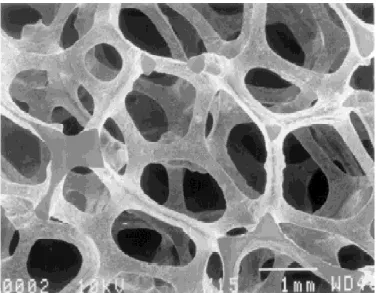
Figure 6 Scanning electron micrograph of ERG Duocel aluminum foam... 9
Figure 7 Tetrakaidecahedron unit cell representation of the ERG open-cell foam (Dharmasena et al, 2002) ... 10
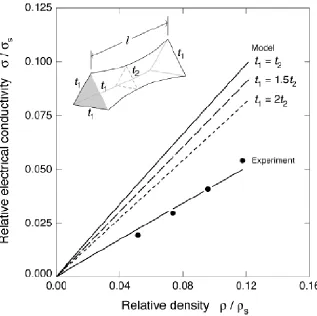
Figure 8 Effect of varying ligament cross section on the electrical conductivity response (Dharmasena et al, 2002) ... 11
Figure 9 Ti-6Al-4V lattice structures made by Electron Beam Melting process ... 13
Figure 10 Micrographs showing the cross section of different ligaments of Ti-6Al-4V hexagonal lattice made on Arcam EBM Machine ... 15
ix
Figure 12 Tetrahedron node ... 16
Figure 13 Schematic representation of cylindrical ligament inscribing tetrahedron node ... 17
Figure 14 (a) Regular hexahedron (b) Equivalent resistive circuit of regular hexahedron .... 18
Figure 15 Regular hexahedron lattice with arrows showing the direction of current when voltage in applied across the uppermost and the lowermost square faces ... 20
Figure 16 (a) Representation of equivalent resistance circuit of regular hexahedron cell (b) Simplified resistance circuit of regular hexahedron ... 22
Figure 17 (a) Octahedron (b) Octahedron lattice ... 24
Figure 18 Octahedron lattice depicting the presence of an extra octahedron unit cell (blue) perfectly fitting in the void in between 8 adjacent unit cells only six of which shown here .. 25
Figure 19 Effective unit cell volume occupied (yellow and blue boxes) by octahedron lattice for conductivity modeling ... 26
Figure 20 Simplified resistance circuit of octahedron ... 27
Figure 21 (a) Truncated octahedron (b) Truncated octahedron lattice ... 29
x
Figure 23 (a) Perspective view and (b) Top view of Truncated Octahedron lattice showing
the effective unit cell (yellow box) ... 31
Figure 24 Simplified resistance circuit of truncated octahedron ... 33
Figure 25 (a) Rhombic Dodecahedron (b) Rhombic Dodecahedron lattice ... 35
Figure 26 Effective unit cell volume (yellow box) in Rhombic Dodecahedron lattice ... 36
Figure 27 Simplified resistance circuit of a rhombic dodecahedron ... 37
Figure 28 (a) Hexagonal Lattice (b) Hexagonal lattice of Ti-6-4 made by EBM Process ... 39
Figure 29 Direction of current in Hexagonal Lattice (arrows showing the direction of current and blue boxes showing effective unit cells) ... 40
Figure 30 Equivalent circuit of Hexagonal lattice ... 41
Figure 31 Relationship between relative conductivity and relative density of foam at low foam density ... 47
Figure 32 Relationship between relative conductivity and ligament length of foam for constant radius of ligament of 0.1mm... 48
Figure 33 Relationship between relative conductivity and radius of ligament of foam for constant length of ligament of 2mm ... 49
xi
Figure 35 Relationship between relative density and ligament length of foam at low density for constant ligament radius of 0.1 mm ... 51
Figure 36 Hexagonal Ti-6Al-4V lattice structures used for resistivity calculation ... 53
Figure 37 Four point probe method for measuring the electrical resistivity of lattice structure ... 54
Figure 38 Comparison of predicted electrical conductivity-relative density relationship (blue line) with experimental results (red square) and error bar of Ti-6Al-4V hexagonal lattice ... 57
Figure 39 Comparison of predicted electrical conductivity-relative density relationship (blue line) with experimental results (red square) and error bar of Ti-6Al-4V Rhombic Dodecahedron lattice ... 58
Figure 40 Electrical resistance heater ... 60
Figure 41 Multi stage heater (Cookson et al, 2006) ... 64
Figure 42 Relationship between radius of ligament and radius of resistive foam ring for constant ligament length to obtain uniform resistance in radial direction ... 65
1
1
INTRODUCTION
1.1
Background
Electrical properties of metal foams have been of interest to researchers studying catalyst support structures (Liu et al, 1999; Liu et al, 2000), high efficiency energy storage applications (Ma et al, 2005; Goodall et al, 2006), and the conversion of electrical to thermal energy (Cookson et al 2006). The electrical conductivity of foams plays an important role in applications involving structural foam enclosures, insulating coatings, protective domes for radar guidance systems and in the mounting of electronic components. An improved understanding of electrical conductivity of foam will enable optimization of the foam properties with respect to the requirements of the application.
2
lattice structures have started receiving a tremendous amount of interest in the research community.
In the first part of this study, the electrical conductivity of five different cell geometries viz. regular hexagon, octahedrons, truncated octahedrons, rhombic dodecahedrons and hexagonal lattice, have been calculated, analyzed and compared. A simplified electrical resistor network derived to model current flow through the foam is taken based on effective unit cell approach. The current path is analyzed and based on the path; the effective unit cell volume is calculated for different cell geometries, which takes care the cells not conducting or voids.
3
1.2
Research Objectives
The first part of this research work aims at comparing the effective resistance for various shapes of non- stochastic lattice structures. The shapes of unit cell of lattice structure considered are Regular Hexahedrons, Octahedrons, Truncated Octahedrons, Rhombic Decahedrons and Hexagonal lattice. For all the shapes the relative density and relative conductivity is calculated using effective unit cell approach. A relationship between the electrical conductivity and ligament radius, ligament length and relative density is obtained. An analysis is done of the electrical conductivity prediction of different shapes and its dependence on shape and density. To validate the analysis, the electrical conductivity of Ti-6Al-4V rhombic dodecahedron and hexagonal lattice made by EBM Process is measured for a range of density varying over 3% to 21%.
4
2
LITERATURE REVIEW
2.1
Applications of Electrically Conductive Metal Foams
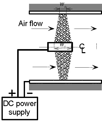
Nickel and copper foams have seen increasing uses as materials of choice for foam-based electrodes. Commonly used electrical resistance heating materials such as iron-foam-based alloys (Fe-Cr-Al), nickel-based alloys (Ni-Cr), carbon compounds, cermets (MoSi2), silicon carbide (SiC), tungsten, molybdenum, and platinum are also used as electrical resistance heater materials. Cookson et al. (2006) studied an electrical resistive heater disk (Fig 1) made of Fe-Cr-Al alloy with potential application as a room heater, a particulate filter for diesel engine exhaust after-treatment, and as a cleaner of airborne biological and chemical agents. An advantage of using resistive mesh structures is that they can be self cleaned via a process of „regeneration‟ in which high current is passed though the metal foam to burn up the captured foreign particles.
5
Figure 1 Configuration of the metal foam electrical air heater (Cookson et al, 2006)
6
7
2.2
Electrical Conductivity of Metal Foams
While mechanical and thermal properties of metal foams have been studied at great length, there has been relatively little evaluation of the electrical properties of non-stochastic cellular structures. The transport properties of closed and open cell foams have been modeled in different ways. Closed cell foams have been modeled and analyzed as two-phase composites involving a continuous solid phase and a continuous or discontinuous gas phase (Wu et al, 2007; Lu et al, 1999). Open cell foams have been approximated using regular polyhedron cell geometries and have been simplified as networks of parallel series resistance elements (Liu et al, 1999; Dharmasena et al 2002; Dukhan et al, 2005; Goodall et al, 2006).
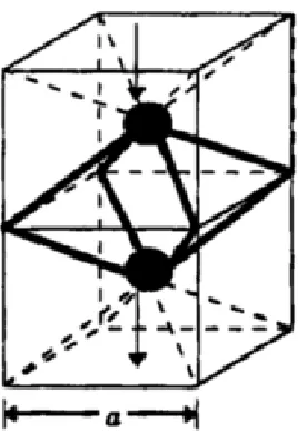
Liu et al (1999) took an octahedron unit cell approach (Fig. 4) for highly porous nickel foams and simplified the unit cell as a network of series and parallel resistors. The relationship derived between resistivity and porosity is given by
1
2 3
1 0.121(1 ') .
1 o
(2.1)
8
Figure 4 Schematic diagram of the octahedron cell geometry (Liu et al, 1999)
9
Dharmasena et al (2002) took a truncated octahedron model of aluminum foams (Fig. 6 and Fig. 7) and treated the metal foam as a network of series and parallel resistors to obtain the apparent electrical conductivity of lower density foams. The ligaments were assumed to have triangular cross sections, and the area was allowed to increase linearly from the middle to its two ends. Nodes were assumed to be tetrahedral, which gave a linear relation between relative conductivity and density as shown in Equations 2.2 and 2.3.
10 2 2 1 2 2 2 1 2 2 0.4082 ln app s t t l t t
(2.2)
3
2 2
1 2 1
2
0.2296 0.0625
s
t t t
l l
(2.3)
where ρ is the density of foam, ρs is the density of the base material, σapp is theapparent conductivity and σ is the electrical conductivity of the base material, t1 is the edge length of the ligament at corner and t2at middle, and l is the length of the ligament.Experimentation showed some deviations (Fig. 8) due to the stochastic nature of the metal foam.
11
One shortcoming of the modeling approach is the inaccurate resistance distribution. The mass of ligaments which were shared between adjacent cells were appropriately considered in density calculation, but their resistance was not assigned accordingly. If a ligament is shared between 2 cells, its mass taken in unit cell approach is half, but the resistance should be doubled since the area became half.
12
2.3
Statement of Need
13
3
CONDUCTIVITY MODEL & CALCULATIONS
The shape of open-cell metal foams have typically been approximated as truncated octahedrons (Dharmasena et al, 2002) which ensures that all the nodes and ligaments of any unit cell are also a part of its adjacent cells when conductivity is calculated. This may not be the case with non-stochastic lattice structures, hence electrical conductivity calculation of the lattice structures differ for cell geometries. In this research, the electrical conductivity of five different cell geometries has been calculated. Since the conductivity and relative density depends on the orientation of the unit-cell in relation to the adjacent cells, the points of contact between adjacent unit cells are very important when modeling. Here the symmetry of unit-cells about an axis has been utilized to simplify the equivalent resistance circuit and hence further calculations.
14
Dharmasena and Wadley (2002) have analyzed stochastic foam, for clarity the same term and approach is employed for the evaluation non-stochastic structures. Non-stochastic lattice structures made by SFF processes (Fig. 9) have ligaments that can be approximated as cylinders with circular cross sections (Fig. 10) hence the ligaments are assumed to be cylindrical. In most of the regular polyhedrons nodes are the meeting point of either 3 or 4 ligaments (Fig. 11); hence nodes can be approximated to tetrahedron (Fig. 12). Assuming the length of a cylindrical ligament is l with radius r and tetrahedral of length t as shown in Figure 11, the volume of a ligament, V1, is given by,
2
Vl r l (3.1)
The cross sectional area Alis given by,
2 l
A r (3.2)
The cylindrical ligament inscribes the tetrahedron, since the cylindrical ligament fits into one of the faces of the tetrahedral (Fig. 13). Hence, the tetrahedral edge t is given by,
2 3
t r (3.3)
The volume of a tetrahedral node, Vn, is given by,
3 3
2
2 6 12
n
15
(a)
(b)
16
(a) (b)
Figure 11 Orientation of (a) three ligaments and (b) four ligaments meeting at the tetrahedron node
17
Figure 13 Schematic representation of cylindrical ligament inscribing tetrahedron node
For calculating the electrical resistance of the unit cell, it is analyzed as a network of series and parallel resistors. For a ligament of constant cross section area (A) and resistivity (rs), the ligament resistance R is given by
. s
l r l R
A
(3.5)
18
3.1
Electrical Conductivity in Regular Hexahedrons
(a) (b)
Figure 14 (a) Regular hexahedron (b) Equivalent resistive circuit of regular hexahedron
A regular hexahedron (Fig. 14a) or cube has 6 faces, 12 ligaments and 8 nodes. The close packed lattice looks like Fig. 14(b). The orientation of the lattice block with respect to the applied voltage determines the path current will follow through each individual unit-cell. Although any orientation is possible, the potential drop in this research is assumed to be applied across any pair of opposing square faces. When voltage is applied across opposite square faces, the current flow is as shown in Fig. 15a. The potential at the ends of horizontal ligaments is identical; hence current does not flow laterally through horizontal ligaments.
19
cell also has 8 nodes whose mass is divided between 8 adjacent cells. The mass of metal in each effective unit cell, Mc, is therefore given by
12 8
3
4 8
c s l n s l n
M V V V V
(3.6)
where ρs is the bulk density of the material from which the lattice is fabricated. The volume of the effective unit cell, Vc, is given by:
3 c
V l (3.7)
From Equations (3.1), (3.4), (3.6) and (3.7), the density of the cellular material ρ can be calculated as:
2 33
3 r 2 6
3 s
s l n
c
c c
l r
V V M
V V l
(3.8)
After rearrangement of terms, the relative density of the cellular material with respect to the bulk material is given by:
2 3
2 3
3 r 2 6
s r l l
(3.9)
The simplified resistive circuit representation is shown in Figure 16, which on further simplification gives the equivalent resistance (Req) between planes 1-2-3-4 and 5-6-7-8 as:
eq
20
Figure 15 Regular hexahedron lattice with arrows showing the direction of current when voltage in applied across the uppermost and the lowermost square faces
If the volume occupied by the effective unit cell is replaced by a homogeneous conductor of the same equivalent resistance,
app eq
eq r .a R =
21
where rappis the apparent resistivity of the equivalent homogeneous solid, a is the distance between two parallel square faces of the regular hexahedron and Aeq is the average unit-cell cross-sectional area. From the geometric relationship for regular hexahedrons,
al (3.12)
3 2 c eq V l A l a l
(3.13)
Electrical resistivity is defined as the inverse of electrical conductivity. From Eq. (3.10), (3.11), (3.12) and (3.13), the apparent electrical conductivity σapp is therefore given by:
2
1 1 1
. app
app
l
r R l Rl
(3.14)
For a ligament of constant cross section, substituting Eq. (3.2) & (3.5) into (3.14)
2 2 1 . app l s s r A
r l r l
(3.15)
The relative conductivity for a cellular material with respect to the bulk material is given by:
2 app s r l
(3.16)
22
4R 4R
4R 4R
4R 4R
4R
4R
4R
4R
4R 4R
1
2
3 4
6
7 8
5
(a)
1
2
3
4
7
6
5
8
4R 4R 4R
4R
(b)
23
cases, the last term in Eq. (3.9) can be ignored. Therefore combining Equations (3.9) and (3.16) gives:
.
3 3
app
s s s
(3.17)
24
3.2
Electrical Conductivity in Octahedrons
An octahedron has 8 faces, 12 ligaments and 6 nodes as shown in Figure 17(a). The orientation of an octahedron unit cell in a close packed lattice (Fig. 17b) gives space for an extra cell to perfectly fit in between 8 adjacent cells (Fig. 18). Since the ligaments of this extra octahedron cell are already a part of the 8 cells surrounding it, it can be treated as a void when modeling electrical conductivity. In the orientation (Fig. 17a) where electrical current enters from the topmost node and exits via the bottommost node, the effective unit cell contains 8 full ligaments, 4 ligaments whose mass is evenly divided between two cells, 2 full nodes, and 4 nodes whose mass is evenly divided between four cells.
(a) (b)
25
Figure 18 Octahedron lattice depicting the presence of an extra octahedron unit cell (blue) perfectly fitting in the void in between 8 adjacent unit cells only six of which shown here
The mass of metal in each effective unit cell, Mc, is therefore given by
1 1 1
.4 8 .4 .2 10 2
2 4 2
c s l n s l n
M V V V V
(3.18)
The effective volume Vc of the octahedron is the volume of a cubic box occupied by a unit cell (Fig. 19) rather than the geometrical volume of an octahedron.
3
2 c
26
Figure 19 Effective unit cell volume occupied (yellow and blue boxes) by octahedron lattice for conductivity modeling
From equations (3.1), (3.4), (3.18) and (3.19) the density of the foam ρ can be calculated as
2 33
10 r l 4 6
10 2
2 s
s l n
c
c c
r
V V
M
V V l
(3.20)
The relative density of foam is given by
2 3 2 3
3
3 2
10 r l 4 6 10 r 4 3
2 2 s r r l l l
27
Fig. 19 shows the simplified resistive circuit for the orientation of octahedron taken, which upon further simplification (Fig. 20) gives equivalent resistance as:
e R
2 q
R
(3.22)
1
2
3
4
7
6
5
8
R R R
R
R R
R R
Figure 20 Simplified resistance circuit of octahedron
If the volume occupied by the effective unit cell is replaced by a homogeneous conductor of the same equivalent resistance, then
e
.
R q app
eq r a
A
28
Where rapp is the apparent resistivity of the equivalent homogeneous solid, a is the height of a unit cell for the given orientation (Fig. 19) and Aeq is the average unit-cell cross-sectional area. From geometric relationship for a regular hexahedron,
2
a l (3.24)
2 eq
A l (3.25)
The apparent electrical conductivity σapp is given by
2
1 2 2 2 2
. app
app
l
r R l Rl
(3.26)
2 1
2
2 2 2 2
. app
s s
r A
r l r l
(3.27)
The relative conductivity for a cell with ligaments of uniform cross section is given by
2 2 2 app s s r r l
(3.28)
For low density metal foam having r<<l
8.8857 2
. 0.4
10 app
s s s
29
3.3
Electrical Conductivity in Truncated Octahedrons
A truncated octahedron has 14 faces, 36 ligaments and 24 nodes as shown in Figure 21(a). In a close packed truncated octahedron lattice (Fig. 21b), considering the orientation where voltage is applied across the two opposite facing square faces, the direction of current flow is as shown in Figure 22. The effective unit cell is a box as shown in Figure 23 incorporating the volume taken by adjacent unit cells not contributing to the electrical conductivity. Hence the effective unit cell contains 12 full ligaments, 24 ligaments whose mass is equally divided between two adjacent truncated octahedrons, and 24 nodes whose mass is equally divided between two adjacent truncated octahedrons.
(a) (b)
30
Figure 22 Truncated octahedron lattice showing current flow (black arrow). The centrally located unit cell (blue) does not contribute to the conductivity model as no current passes
through it
The mass of metal in each effective unit cell, Mc, is therefore given by:
24 24
12 24 12
2 2
c s l n s l n
M V V V V
31
(a)
(b)
32 The unit cell volume Vc is given by
3
18 2 c
V l (3.31)
From Equations (3.1), (3.4), (3.30) and (3.31), the density of the foam ρ can be calculated as
2
3
s
s l n
c
3
c c
24 r l + 2 12 6r 24V +12V
M
= = =
V V 18 2l
(3.32)
Hence,
2 3
2 3
3 2 3
24 r 24 6 24 r 24 6
18 2 18 2 18 2
s
l r r
l l l
(3.33)
For the orientation considered, the simplified resistance circuit is given by Figure 24, which upon further simplification yields:
e
R q R (3.34)
If the volume occupied by the effective unit cell is replaced by a homogeneous conductor of the same equivalent resistance, then we have:
e
.
R q app
eq r a
A
(3.35)
From geometric relationship for regular hexahedron,
2 2
a l (3.36)
3 2 18 2 9 2 2 c eq V l A l a l
33
1 2 3 4
2R 2R 2R 2R R 7 6 5 8 R R 2R 2R 2R 2R R 2R 2R R 2R 2R 2R 2R R 2R 2R R
Figure 24 Simplified resistance circuit of truncated octahedron
From Eq. (3.34), (3.35), (3.36) and (3.37), the apparent electrical conductivity σapp is given by
2
1 1 2 2 2 2
.
9 9
app app
l
r R l Rl
(3.38)
For a ligament of constant cross section, substituting Eq. (3.2) & (3.5) into (3.38)
2
2
2 2 2 2
9 . 9
app 1
s s
r A
r l r l
(3.39)
The relative conductivity for a cell with ligaments of uniform cross section is given by:
2 2 2 9 app s r l
34 For low density foams (r<<l)
2 2
9 .
24 3
18 2 app
s s s
35
3.4
Electrical Conductivity in Rhombic Dodecahedrons
(a) (b)
Figure 25 (a) Rhombic Dodecahedron (b) Rhombic Dodecahedron lattice
A rhombic dodecahedron has 12 faces, 24 ligaments and 14 nodes (Fig. 25a). In a close packed lattice (Fig. 25b), the effective unit cell contains 8 full ligaments, 16 ligaments whose mass is evenly shared between two adjacent cells, 10 half nodes whose mass is evenly shared between two adjacent cells and 4 nodes whose mass is evenly shared between four adjacent cells (Fig. 26). The mass of material in each effective unit cell, Mc, is therefore given by
16 10 4
8 16 6
2 2 4
c s l n s l n
M V V V V
36
Figure 26 Effective unit cell volume (yellow box) in Rhombic Dodecahedron lattice
3 6.1581 c
V l (3.43)
From Equations (3.1), (3.4), (3.42) and (3.43) the density of the foam ρ can be calculated as
2 33
16 12 6
16 6
6.1581 s
s l n
c
c c
r l r
V V
M
V V l
(3.44)
37
2 3
3
16 12 6
6.1581 s
r l r
l (3.45) 2R 2R 2R 2R R R R 2R 2R 2R 2R R 2R 2R 2R 2R 2R 2R R R R 2R 2R R
Figure 27 Simplified resistance circuit of a rhombic dodecahedron
From Figure 27, we have:
e
R q R (3.46)
If the volume occupied by a effective unit cell is replaced by a homogeneous conductor of the same equivalent resistance, then
e
.
R q app
eq r a
A
(3.47)
38 2.3094
a l (3.48)
3 2 6.1581 2.6665 2.3094 c eq V l A l a l
(3.49)
From Eq. (3.46), (3.47), (3.48) and (3.49), the apparent electrical conductivity σappis given by
2
1 1 2.3094 0.8661
.
2.6665 .
app app
l
r R l R l
(3.50)
For a ligament of constant cross section, substituting Eq. (3.2) & (3.5) into (3.50)
2 2
1 2
0.8661 0.8661 2.7209
. app
s s s
r r
A
r l r l r l
(3.51)
2 2.7209 app s r l
(3.52)
For very low density foams (r<<l)
2.7209 .
8.162 3
app
s s s
39
3.5
Electrical Conductivity in Hexagonal Lattices
(a) (b)
Figure 28 (a) Hexagonal Lattice (b) Hexagonal lattice of Ti-6-4 made by EBM Process
A hexagonal lattice as shown in Figure 28 has 12 ligaments and 10 nodes. In the orientation where voltage is applied across the topmost and bottommost nodes (Figure 28a and Figure 29), an effective unit cell contains 4 full ligaments, 8 ligaments whose mass is evenly shared by two adjacent cells, 6 nodes whose mass is evenly shared by two adjacent cells, and 4 nodes whose mass is evenly shared by four adjacent cells. The mass of material in effective unit cell, Mc, is therefore given by
8 6 4
4 8 4
2 2 4
c s l n s l n
M V V V V
40
Figure 29 Direction of current in Hexagonal Lattice (arrows showing the direction of current and blue boxes showing effective unit cells)
The effective unit cell volume Vc is given by
3 6 c
V l (3.55)
From equations (3.1), (3.4), (3.54) and (3.55) the density of the foam ρ can be calculated as
2 31
3
8 8 6
8 4
6 s
s n
c
c c
r l r
V V
M
V V l
41 Hence
2 3
3
8 8 6
6 s
r l r
l
(3.57)
From Figure 30 Req 2R (3.58)
1
2
2R
R 2R
R
R 2R
2R R
2R
2R
2R 2R
Figure 30 Equivalent circuit of Hexagonal lattice
42
e
.
R q app
eq r a
A
(3.59)
From geometric relationships for a, effective unit cell in hexagonal lattice,
2
a l (3.60)
3 2 6 3 2 c eq V l A l a l
(3.61)
From Eq. (3.58), (3.59), (3.60) and (3.61), the apparent electrical conductivity σappis given by
2
1 1 2 1
.
2 3 3
app app
l
r R l Rl
(3.62)
For a ligament of constant cross section, substituting Eq. (3.2) & (3.5) into (3.62)
2 1 2 1 3 3 app s s r A
r l r l
(3.63)
The relative conductivity for a cell with ligaments of uniform cross section is given by
2 3 app s r l
(3.64)
For very low density metal foams (r<<l)
1.0471
. 0.2499
4.1888 app
s s s
43
4
ANALYSIS AND VALIDATION
The preceding chapter presented a number of different unit cell geometries. For each cell geometry, a variety of geometric and electrical properties were analytically derived as a function of the unit cell size and shape. In this chapter, those equations are used to compare expected performances of lattice structures fabricated in different sizes and shapes. In order to validate the analytical models, the electrical performance of four different size hexagonal lattice structures was experimentally measured. The predicted conductivity and measured conductivity were then compared.
4.1
Shape and Density Dependency of Lattice Structures
44
Table 1 Physical properties of Various Unit Cell Geometries
Shape Fac es L igame n ts Ve rtic es Height of unit- cell (a)
Effective Unit-cell Volume (Vc)
Equivalent Resistance
(Req)
Regular
Hexahedron 6 12 8 l
3
l Rl
Octahedron 8 12 6 2l 3
2l
2 l R Truncated
Octahedron 14 36 24 2 2l 18 2l3 Rl
Rhombic
Dodecahedron 12 24 14 2.3094l
3
6.1581l Rl
Hexagonal
Lattice - 12 10 2l
3
6l 2Rl
Table 2 summarizes electrical properties of the five different lattice structures described in the previous chapter. In all cases, the ligament has been assumed to be perfectly cylindrical. Likewise, the nodes are assumed to be tetrahedral. The effective unit cell approach used gives a more accurate estimate of the electrical conductivity of the lattice due to the fact that voids are taken into consideration. A void is the volume enclosed by ligaments which are a part of another cell (e.g. the blue octahedron in Fig. 18).
45
Table 2 Electrical Properties of Various Unit Cell Geometries
Shape Relative Density* s Relative Conductivity app s app s s * Regular Hexahedron 2 3 r l 2 3.1416 r l
0.3333
Octahedron 2 10 2 r l 2 8.8857 r l
0.4
Truncated Octahedron 2 2.9616 r l 2 0.9873 r l
0.3333
Rhombic Dodecahedron 2 8.162 r l 2 2.7209 r l
0.3333
Hexagonal Lattice 2 4.1888 r l 2 1.0471 r l
0.2499
*For low density metal foams where r<<l
for a given relative density. The value of the ratio of relative conductivity to relative density indicates the dependence of electrical conductivity on the cell geometry.
46
hexahedron, yet the conductivity of each cell type is identical for a given density. Hence a regular hexahedron lattice will have the same conductivity as a rhombic dodecahedron or octahedron lattice. However, it is advantageous where space is constraint as it occupies least volume. Regular hexahedrons and octahedrons have the same number of ligaments, yet they have different relative conductivities for a given relative density. This indicates that electrical conductivity is most definitely shape dependent.
47
Figure 31 Relationship between relative conductivity and relative density of foam at low foam density
0 0.02 0.04 0.06 0.08 0.1 0.12 0.14
R
el
a
ti
v
e
C
o
nducti
v
ity
Relative Density
Regular Hexahedron Octahedron
48
Figure 32 Relationship between relative conductivity and ligament length of foam for constant radius of ligament of 0.1mm
0 0.005 0.01 0.015 0.02
2.1 2.2 2.3 2.4 2.5 2.6 2.7 2.8 2.9 3 3.1 3.2 3.3 3.4 3.5 3.6 3.7 3.8 3.9 4 4.1 4.2
R
el
a
ti
v
e
C
o
nducti
v
ity
Length of Ligament (mm)
Regular Hexahedron Octahedron
49
Figure 33 Relationship between relative conductivity and radius of ligament of foam for constant length of ligament of 2mm
0 0.05 0.1 0.15 0.2 0.25
0.1 0.12 0.14 0.16 0.18 0.2 0.22 0.24 0.26 0.28 0.3
R
el
a
ti
v
e
C
o
nducti
v
ity
Radius of Ligament (mm)
Regular Hexahedon Octahedron
50
Figure 34 Relationship between relative density and radius of ligament of foam at low density for constant value of ligament length of 2mm
0 0.005 0.01 0.015 0.02 0.025 0.03 0.035 0.04 0.045 0.05 0.055
2.1 2.3 2.5 2.7 2.9 3.1 3.3 3.5 3.7 3.9 4.1
R
el
a
ti
v
e
dens
ity
Length of Ligament (mm)
Regular Hexahedron Octahedron
51
Figure 35 Relationship between relative density and ligament length of foam at low density for constant ligament radius of 0.1 mm
0 0.1 0.2 0.3 0.4 0.5 0.6
0.1 0.12 0.14 0.16 0.18 0.2 0.22 0.24 0.26 0.28 0.3
R
el
a
ti
v
e
D
ens
ity
Radius of Ligament (mm
) Regular HexahedronOctahedron
52
4.2
Experimental Validation
To validate the conductivity models and findings, experiments were performed to obtain the resistivity of the rhombic dodecahedron and hexagonal lattice structures at three and four different densities respectively. Four hexagonal lattice structures of different ligament length but identical ligament radius were designed using the Solid Works CAD package. The ligament radius taken was 0.35 mm and the different ligament lengths considered were 1.72mm, 2.31mm, 2.89mm, and 3.45mm respectively (~0.07, 0.09, 0.11, 0.14 inches). Four titanium alloy Ti-6Al-4V hexagonal lattice structures having overall dimensions of 190mm x 28mm x 28mm (7.5" x 1.1" x 1.1") were fabricated on an ARCAM A2 Electron Beam Melting (EBM) machine (Fig. 36). Ti-6Al-4V is the most widely used of all titanium alloys with many aerospace, industrial and medical applications. Similarly, rhombic dodecahedron lattices were designed and fabricated via the EBM process. The fabricated samples have a constant ligament length (3.72 mm) and different ligament radii of 0.67mm, 0.92mm and 1.26mm.
The mass of the individual structures were obtained on an electronic balance, and the bounding box volumes of the individual samples were calculated following measurement of
the lattice block's external dimensions. The ratio of mass to volume gave the density. The relative density was obtained by dividing the lattice sample density by the bulk density of
53
was measured using a four-point probe method shown in Figure 37. The four-point probe
Figure 36 Hexagonal Ti-6Al-4V lattice structures used for resistivity calculation
method is useful for measuring resistivity of material by contact with its surface; since it neglects the probe resistance and probe contact resistance.
54
1 3 1 2 2 3
2
1 1 1 1
V I r
S S S S S S
(4.1)
where V is the potential drop across points P2 and P3, I is the current injected through point P1, and S1, S2, S3 are the respective distances between probes P1-P2, P2-P3, P3-P4.
Figure 37 Four point probe method for measuring the electrical resistivity of lattice structure
A constant current of 2 Amp was passed through all the lattice structures separately using a NULINE DC Power supply CED 936. The voltage drop between the inner two probes was measured using a FLUKE 87 TRUE RMS Multimeter.
55
relative conductivity calculations for the four hexagonal lattice structures are also provided. Figure 38 and Figure 39 compares the predicted and measured values for relative density versus relative conductivity for the hexagonal and rhombic dodecahedron samples respectively. Compared with prior research in which predicted resistivity for stochastic foams were compared with actual resistivity, it can be said that the agreement between the predicted and actual resistivity for the hexagonal lattices are quite good. One possible reason for the slight variation in the experimental data and the conductivity prediction is due to the presence of sintered powder on surface of the ligament (Fig. 10) resulting in the increase of area for conduction.
56
Table 3 Calculation of relative electrical conductivity of Ti-6-4 hexagonal lattice structures based on experimental data (averaged over four readings for each ligament length)
Ligament Length (mm) Relative Density Average Resistivity (Ω mm) Average Relative Resistivity s Average Relative Conductivity app s app s s
3.453 0.034 0.174 102.403 0.009 0.288
2.896 0.054 0.109 64.002 0.016 0.291
2.311 0.078 0.072 42.668 0.023 0.299
1.727 0.126 0.056 32.822 0.030 0.242
Table 4 Calculation of relative electrical conductivity of Ti-6-4 rhombic dodecahedron lattice structures based on experimental data (averaged over four readings for each ligament
radius) Ligament Radius (mm) Relative Density Average Resistivity (Ω mm) Average Relative Resistivity s Average Relative Conductivity app s app s s
0.67 0.057 0.135 79.789 0.013 0.219
0.92 0.106 0.070 41.372 0.024 0.228
57
Figure 38 Comparison of predicted electrical conductivity-relative density relationship (blue line) with experimental results (red square) and error bar of Ti-6Al-4V hexagonal lattice
0 0.005 0.01 0.015 0.02 0.025 0.03 0.035 0.04
0 0.02 0.04 0.06 0.08 0.1 0.12 0.14 0.16
R
el
at
ive
C
ond
uct
ivi
ty
Relative Density
Experimental data
58
Figure 39Comparison of predicted electrical conductivity-relative density relationship (blue line) with experimental results (red square) and error bar of Ti-6Al-4V Rhombic
Dodecahedron lattice
0 0.01 0.02 0.03 0.04 0.05 0.06 0.07 0.08
0 0.05 0.1 0.15 0.2 0.25
R
el
at
ive
C
ond
uct
ivi
ty
Relative Density
59
5
ELECTICAL CONDUCTIVITY IN VARIABLE DENSITY
LATTICE STRUCTURES
5.1
Modeling and Calculations
The notion of varying the density in metal foams has received little attention to date due to limitations with the conventional methods of fabrication. However Solid Freeform Fabrication (SFF) techniques provide enormous flexibility when it comes to designing and fabricating lattice structures in which density can be spatially varied. By varying the density from one location to another within a structure, designers can customize the material properties of the lattice based on the functional requirements of the application. Hence structural, acoustic (sound), electrical and thermal properties of non-stochastic cellular structures can be varied according to the needs of the application.
Cookson et al. (2006) described an electrical resistance heating application in which variable foam density would be advantageous. The electrical current flows through a metal foam disk, which serves as the heating element, between an outside tube and an inner center rod as shown in Figure 40. The shortcoming of the electrical resistance heater is that it has more resistance towards the center than it does towards the periphery, which results in uneven heat generation and transfer to the air flowing through the heater (Fig. 2).
60
radius of αi and outer radius of αo. Following the analysis of Cookson et al. (2006), let the resistance of the ring in the radial direction be Rr.
r s d R A (5.1)
where ρs is the electrical resistivity of the material and A=2παw is the circumferential area of the ring.
Figure 40 Electrical resistance heater
Integrating Eq. (5.1) to obtain the resistance of the ring, gives (Cookson et al., 2006)
ln 2 2 o i o ring i d R w w
(5.2)61 ( ) o i o i ring
o i o i
d R w w
(5.3)Eq. (5.3) clearly explains the reason for the decrease in resistance as the radius of the ring increases. This decrease in the resistance as the radius increases can be overcome by increasing the relative density of the foam. In other words, a metal foam disk with increasing relative density as the radial distance from the central axis increases can be designed such that a constant electrical resistance is achieved. This, in turn, will yield uniform heat generation. To determine the rate at which density should be increased to maintain uniform electrical resistance, let us assume that a metal foam disk has an inner radius of αi , a ligament length of lo, and a radius of ro.
Assuming a regular hexahedron unit cell (Eq. 3.16), the resistance of a ring having a unit cell thickness at radius α, ligament length l, and radius r is given by:
2 2
0.3183
2 2
lr app s
a l l
R
w r w
(5.4)
Where a is the height of the unit cell and w is the width of the foam disk. Further equating the resistance of the ring at radius α of the disk (Fig. 40) to the resistance of the innermost row (radius αo, ligament length lo, radius ro)
Rlr Ro o ol r
Gives 3 3 2 2 1 1 0.3183 0.3183 2 2 o s s o o l l
r w r w
62
3 3
2 2
o
o o l l
r r
(5.5)
Equation 5.5 gives the relation between the ligament length and radius at different distance from the center of the ring. Uniform resistance can be obtained by varying either the ligament length or ligament radius or both.
63
5.2
Analysis of a Variable Density Application
Variations in density can enhance the efficiency and performance of non-stochastic cellular structures. Here an application is explained to enhance the working of an electrical resistance heater. A disk shape heater whose potential applications could include household or office space heaters and particulate filtration for diesel engine exhaust after treatment. The circular shape of the heater facilitates its fitting into pipes. At the same time, its disadvantage is that the electrical resistance is greater at the center and decreases in radial direction. Heating is therefore uneven. The alternative suggested by Cookson et al. (2006) is to decrease the thickness of the foam disk in the radial direction. However under constant flow rate, this will reduce the residence time of air in the foam, thus reducing heat transfer. This problem can be mitigated by keeping several disks (Fig. 41) of foam in series (Cookson et al, 2006). This process may not be very efficient when used for particulate filtration, since the efficiency of the disc will be higher at the center, decreasing in radial direction.
64
Figure 41 Multi stage heater (Cookson et al, 2006)
65
Figure 42 Relationship between radius of ligament and radius of resistive foam ring for constant ligament length to obtain uniform resistance in radial direction
0 0.2 0.4 0.6 0.8 1 1.2
11 12 13 14 15 16 17 18 19 20 21 22 23 24 25 26 27 28 29 30 31
R
adius
of
L
igam
ent
(
m
m
)
Radius of resistive foam ring (mm)
ro= 1 mm
ro= 0.75 mm
ro= 0. 5 mm
66
Figure 43 Relationship between length of ligament and radius of resistive foam ring for constant ligament radius to obtain uniform resistance in radial direction
0 0.5 1 1.5 2 2.5 3
11 12 13 14 15 16 17 18 19 20 21 22 23 24 25 26 27 28 29 30 31
L
engt
h
of
L
igam
ent
(
m
m
)
Radius of the resistive ring (mm)
lo= 2 mm
lo= 1.75 mm
lo= 1.5 mm
67
6
CONCLUSIONS AND RECOMMENDATIONS
6.1 Conclusion
In this study, the electrical conductivity of 5 different cell geometries (regular hexahedron, octahedron, truncated octahedron, rhombic dodecahedron, and hexagonal lattice) was calculated using an effective unit cell approach and compared along with their relative density at low foam density. The relationship between relative conductivity, relative density, ligament length and radius was established for each cell geometry at a given orientation. The different values of the ratio of relative conductivity to relative density indicate the shape dependence of electrical conductivity.
The octahedron cell geometry was shown to have the highest value of electrical conductivity, while the hexagonal lattice was shown to have the highest resistivity at a given relative density for the orientation considered. At low densities, the relative conductivity of non-stochastic lattice structures increases linearly with increase in relative density. Increases in the ligament length resulted in the decrease of conductivity. Increases in ligament radius led to increases in conductivity. Resistivity measurements of Ti-6Al-4V rhombic dodecahedron and hexagonal lattice structures over a range of relative densities from 3% to 20% made by EBM process validated the effective unit cell approach to predict the conductivity and the fact that electrical conductivity increases on increasing the relative density of foam.
68
69
6.2
Recommendations for future study
This work has only considered regular polyhedrons at particular orientation; though it is quite possible that some non-regular polyhedrons or polyhedrons considered here for different orientation can have different electrical properties. Therefore development of shape optimization algorithms to find the best shape and best orientation possible for a particular application is seen as the next step to this work.
It is assumed during the calculations that the ligaments are cylindrical, but the microstructures of lattice fabricated by SFF processes have very rough surface. This could result in substantial drop in conductivity by producing eddy current. The calculation of this factor for different SFF processes will make the evaluation of conductivity easier.
Electrical conductivity of metal also depends on the degree of sintering. Evaluating the relationship between conductivity and degree of sintering for different metals will be very useful.
No design software is available which can vary the unit cell shape of a lattice parametrically. Development of such software will provide a milestone in the field of varying density of metal foam.
70
REFERENCES
Cookson E.J., D.E. Floyd, A.J. Shih (2006) “Design, manufacture and analysis of metal foam electrical resistive heater” Int. J. Mech. Sci. 48, 1314–1322.doi:10.1016/ j.ijmecsci.2006.05.006
Dharmasena K.P., H.N.G. Wadley (2002) “Electrical conductivity of open-cell metal foams” J. Mater. Res. 17(3), 625–631, doi: 10.1557/ JMR .2002.0089
Dukhan N., P. D. Quiñones-Ramos, E. Cruz-Ruiz, M. Vélez-Reyes and E. P. Scott
(2005) “One-Dimensional Heat Transfer Analysis in Open-Cell 10-ppi Metal Foam,” International Journal of Heat and Mass Transfer, Vol. 48, No. 25-26, pp. 5112-5120.
Gibson L.J., M.F. Ashby (1997) Cellular Solids: Structure and Properties, second ed., Cambridge University Press, pp. 25–37.
Goodall, R., Weber, L., Mortensen, A. (2006) “The electrical conductivity of microcellular metals” Journal Of Applied Physics, vol. 100, num. 4,.
Liu P.S., T.F. Li, C. Fu (1999) “Calculation formula for apparent electrical resistivity of high porosity metal materials” Mater. Sci. Eng., A 268, 208–215. doi:10.1016/S09215093 (99) 00073-8
Liu P.S., H. Chen, K.M. Liang, S.R. Gu, Q. Yu, T.F. Li et al. (2000) “Relationship between apparent electrical-conductivity and preparation conditions for nickel foam” J. Appl. Electrochem. 30, 1183–1186. doi:10.1023/A:1004095410450
Lu TJ, Chen C. (1999) “Thermal transport and fire retardance properties of cellular aluminium alloys”, Acta mater.47, 1469-1485,.
Ma X., A.J. Peyton, Y.Y. Zhao (2006) “ Measurement of the electrical conductivity of open-celled aluminium foam using noon-contact eddy current techniques”, NDT Int. 39, 562– 568. doi:10.1016/j.ndteint.2006. 03.008