A New Approach to Pollen Classification using Computational Intelligence

(1)

ISSN(Online): 2320-9801 ISSN (Print): 2320-9798

I

nternational

J

ournal of

I

nnovative

R

esearch in

C

omputer

and

C

ommunication

E

ngineering

(An ISO 3297: 2007 Certified Organization)

Website:www.ijircce.com

Vol. 5, Issue 1, January 2017

A New Approach to Pollen Classification using

Computational Intelligence

V. R. Dhawale, J. A. Tidke, S. V. Dudul

Asst. Professor and Head, Dept. of MCA, Vidya Bharati Mahavidyalaya, Amravati, Maharashtra, India

Professor and Head, Dept. of Botany, Sant Gadge Baba Amravati University, Amravati, Maharashtra, India

Professor and Head, Dept. of A. E., Sant Gadge Baba Amravati University, Amravati, Maharashtra, India

ABSTRACT: A new classification approach is proposed for pollen grains. Along with image statistics and shape descriptor, histogram (H) coefficient features were used as input to the classifier. As the earlier reported approaches werefound to be tedious and time consuming with less accuracy, the present approach gives precise accuracy in classification of pollen grains by using SEM images. The improved classifiers based on Generalized Feed Forward (GFF) Neural Network, Modular Neural Network (MNN), Principal Component Analysis (PCA) Neural Network, and Support Vector Machine (SVM) are explored with optimization of their respective parameters in view of reduction in time as well as space complexity. In order to reduce the space complexity, sensitivity analysis is done to eliminate theinsignificant parameters from the dataset.As performance of all these neural networks is compared with respect to MSE, NMSE and the Average Classification Accuracy (ACA), GFF NN comprising of two hidden layers is found to be superior (95 % ACA on CV dataset) to all other classifiers. The new improved classifier algorithm with Histogram coefficients provides more accuracy as compared to the earlier algorithms, which usedDiscrete Cosine Transform Features and Walsh Hadamard Transform coefficients. The robustness of the classifier to noise is verified on the Cross validation dataset by introducing controlled Gaussian and Uniform noise in both input and output. The proposed approach is inexpensive, reliable and nearly accurate that can be used without help of experts from the field of palynology.

KEYWORDS: Pollen SEM images,palynology, Computational Intelligence, Multi-layer Perceptron Neural Network, Principal Component Analysis, Support Vector Machine, Classifier.

I. INTRODUCTION

Pollen grains are widely used as fingerprint for classification of plant species. Traditionally, pollen morphological characters are used for plant classification and identification of plants [1]. From the related work reported so far, it is

observed that researchers used neural network for pollen identification and classification. Li et al. [2, 3] identified pollen

grain microstructure using neuralnetworks. Rodriguez-Damian M. et al. [4, 5]employed brightness and shape descriptors

for pollenclassification. Travieso C M.et al.[6] developed contour featurebased classification, which is based on an

HMM kernel and SVMwas used as classifier in that system. P.Carrion et al.[7] hadproposed improved classification of

pollen texture imagesusing SVM and MLP. N R Nguyen et al. [8] proposed an improved pollen classification with less

training effort by introducing new selection criterion to obtain the most valuable training samples. Kalva et al. [9] used

combination of neural network classifier with Naïve Bayes classifier that uses features such as color, shape and texture extracted from web images giving meaningful improvement in the correct image classification rate relative to the results provided by simple neural network based image classifier, which does not use contextual information.

(2)

I

nternational

J

ournal of

I

nnovative

R

esearch in

C

omputer

and

C

ommunication

E

ngineering

Due to availability of SEM high resolution digital images of sample pollen grains showing above prominent characters, they were obtained and used for classification.

The application of Artificial Intelligence methods was reported to develop a classifier, which was earlier designed on the basis of Walsh Hadamard Transform coefficients along with statistical features giving 85% classification accuracy

(CA), Dhawale et al. [11].

The main morphological characters such as shape, size, symmetry, pollen wall, exine stratification and ornamentation were proved to be very important for its study and classification. The shape of pollen grain is an important morphological character. The shape of pollen grain varies in different views, namely, polar view and equatorial view. The outline in polar view is circular, triangular, square shaped, pentagonal, rounded or any other geometrical shape. In the present study, SEM images of pollen samples prominently showinggeometrical shapes such as circular, triangular, rectangular, squared and elliptical were considered. SEM high resolution digital images of sample pollen grains showing above prominent characters were obtained and used for classification.

The application of Computational Intelligence methods like neural networkshas gained popularity in solving pattern

recognition problems. The current study mainly emphasizes on the improved Histogram coefficient based neural

classifier and other computational intelligence technologies.

This image dataset includes ten different plant species, such as, Brassicanigra, Callistemon citrinus, Erythrina

suberosa, Euphorbiageniculata, Gloriosa superba, Impatiens balsamina, Jasmeniumofficinale, Jatropa panduraefolia, Madhuca indica, and Morindatomentose.

A neural network performs pattern classification by first undergoing a training session, during which the network is repeatedly presented a set of input patterns along with the category to which each particular pattern belongs. Later, a new pattern is presented to the network for CV that has not been seen before, but which belongs to the same population of patterns used to train the network. The network is able to identify the class of that particular pattern because of the information it has extracted from the training data. Pattern recognition performed by a neural network is statistical in nature, with the patterns being represented by points in a multidimensional decision space. The decision space is divided into regions, each one of which is associated with a class. The decision boundaries are estimated by the training process. The construction of these boundaries is made statistical by the inherent variability that exists within and between classes. The paper has been organized in four sections comprising of Introduction, Feature Extraction, Experimental Setup, Result and Discussion. Experimental Setup deals with design and development of classifiers based on GFF NN, Modular NN, PCA NN, and SVM.

A. PROCEDURE ADAPTED FOR POLLEN CLASSIFICATION A general flowchart of NN-based classifier is shown in the Fig.1

Fig.1 Flowchart of NN based classifier

(3)

I

nternational

J

ournal of

I

nnovative

R

esearch in

C

omputer

and

C

ommunication

E

ngineering

II.FEATUREEXTRACTION

SEM images captured by Leo – 430 are segmented and cropped by using image processing software in order to get the region of interest (ROI). Cropped images are stored in .jpg format. ROI is located and separated to extract features.

The main issuesregarding the design of NN are the selection of significant inputs and how to choose the NN parameters creating the highly accurate network. Hence, Pollen image is represented by a feature vector F; which is comprised of 128 different parameters. The dataset contains only 51 instances (exemplars) for ten different plant species. Learning from such a small sized data is still considered as a challenging task for neural networks. It is partitioned into training and cross validation or testing dataset. The training dataset constitutes 34 exemplars and the remaining 17 exemplars are used for cross validation or testing.

The improved neural network based classifier is trained from the training dataset, where a feature vector is mapped onto a particular pollen class or name of plant species. The neural network learns from data (trainingexemplars) and the connection weights and biases are estimated as a result of this learning. After training of the neural network, its connection weights are frozen and tested on a different cross-validation (CV) dataset, which was never presented to the neural network. The performance of the classifier based on neural network is evaluated on the basis of some metrics, such as, MSE (Mean Square Error), NMSE (Normalized MSE), ACA and Confusion Matrix. In this work, the prototype model of the classifier is developed with a view to discriminate between 10 different pollen species. However, the proposed algorithm can be easily modified for classification of more than 10 pollen species provided that one has enough computational resources.

The feature vector, which is to be extracted from the separated ROI of pollen image, is as follows.

F=[H128,H129,….,H146,H148,...,H181,H183,…,H192,H194,…,H199,H201,…,H213,H215,…H225,H227,…,H249,H2 51,…,H255, Average, Standard Deviation, Entropy, Contrast, Correlation, Energy, Homogeneity, Shape]; Where H128,…,H255denote the two dimensionaldiscrete Histogram coefficients. The shape descriptor consists of five different softfeatures describing shape of pollen grain such as circular, triangular, rectangular, squared and elliptical.

An image histogram is a type of histogram which acts as a graphical representation of the tonal distribution in a digital image and histogram equalization (HE) is one of the common methods used for improving contrast in digital images. The histogram (H) coefficients were obtained by HE, a technique that aims to maximize the “information efficiency” of the image, in the sense that more frequent pixels should be entitled to a larger intensity range. Surprisingly, the function that does this transformation is cumulative distribution function of the image histogram. This technique is implemented for pollen SEM images, for feature extraction.

To develop an improved algorithm, SEM images of pollen grains of 10 different plant species considered are shown in Fig. 9 at the end of this paper before conclusion. There is a need to come up with a novel feature extraction method toclassify the pollen samples. In addition to histogram (H)coefficients the following statistical features of a pollen SEM images are computed,

1. Average: It indicates two dimensional mean of image matrix.

2. Standard Deviation: Standard deviation of elements contained in image matrix.

3. Entropy: It is a statistical measure of randomness which can be used to characterize the texture of input image. It is

defined as, =− ∑plog ( )

where, p denotes the histogram counts of a pollen image. Image texture provides information about the

spatialarrangement of colour or intensities in an image or selected region of an image. GLCM represents numerical features of a texture using spatial relations of similar gray tones. Numerical features calculated from GLCM can be used to represent, compare and classify textures. From Gray Level Co-occurrence Matrix (GLCM) of an image following parameters (4 to 7) are computed. This matrix shows how often a pixel with gray scale intensity (gray level)

value i occurs horizontally adjacent to a pixel with the value j

4. Contrast: It is defined as separation between the darkest and brightest area of an image. It measures the local variations in the gray level co-occurrence matrix

5. Correlation: It is a measure of how correlated a pixel is to its neighbour over the whole image. It also includes the joint probability occurrence the specified pixel pairs.

(4)

I

nternational

J

ournal of

I

nnovative

R

esearch in

C

omputer

and

C

ommunication

E

ngineering

7. Homogeneity:It is a measure of texture of an image. It measures the closeness of the distribution of elements in the GLCM to the diagonal of GLCM.

8. Shape descriptor: Shapes of the pollen grain images considered are visually inspected and they are identified as oval, rectangular, circular, triangular and elliptical.

Initially, 264 features were computed comprising of 256 H coefficients and 8 other image features. However, with a view to reduce the dimensionality of the input space, a computer simulation experiment has been carried out, where the number of H coefficients are varied from 2 to 256 in the octave, that is, 2, 4, 8, 16, 32, 64, 128 and 256. In each case, a feature vector is generated for a pollen image and a dataset isformed.For 128-element feature vector, the classification performance is the best. It is also noticed that further reduction in the size of the feature vector has deteriorated such a performance. Therefore, it is inferred that the optimal feature vector should contain 128 elements (parameters) for a reasonable performance.

One problem that often arises after feature extraction is,that there are too many input features that would require significant computational efforts and this may result in low classification accuracy. To make potential improvements in ACA,sensitivity analysis is carried out on training as well as CV dataset for identifying the insignificantfeatures in the classifier input and finally 120 H features (numeric valued) were selected along with 7 statistical numeric valued featuresand one symbolic Shape descriptor feature translated into 5 bit binary number. Thus, in order to represent one shape, five binary valued inputs are required. Therefore, total number of input features is 132.

III.EXPERIMENTAL SETUP

Histogram equalization approach is used, where a pollen SEM image is subjected to histogram equalization algorithm through MATLAB code and the results are assembled into an output image. An environment accessible from MATLAB (Mathworks Inc., USA) is used to implement the algorithm that processes the input image resulting in 2D discrete feature extraction.

Neuro Solutions (NeuroDimensions, Inc. USA) 5.07 was used to implement various NN based classifiers on pollen image which is represented by a Feature Vector containing 128 different elements.

In this paper, the performance analysis of classifiers is made by comparing the results of GFFNN, MNN, PCA NN, and SVM based classifiers and they arevalidated and tested meticulously for accuracy and robustness.

(5)

I

nternational

J

ournal of

I

nnovative

R

esearch in

C

omputer

and

C

ommunication

E

ngineering

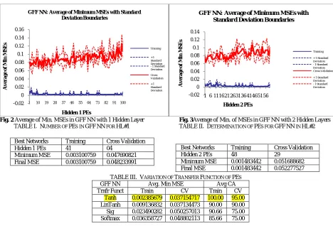
Thus the architecture of the proposed GFF NN is (Input Layer PEs) – (Hidden Layer #1 PEs) – (Hidden Layer #2 PEs) – (Output Layer PEs), i.e. 132-04-29-10. This network has been trained for different transfer functions of PEs in both the hidden layers and as shown in Table III, choice of ‘tanh’ transfer function in both the hidden layers resulted into the best classification performance even on CV dataset.

The selected parameters for GFF NN are given below:

Number of epochs=5000, Exemplars for Training=34, Exemplars for Cross Validation/Testing = 17, Numberof Hidden Layers = 02, Transfer Function: Tanh, Learning Rule: Momentum.

Proposed NN is trained on Training and Cross Validation datasets. The performance of NN is tested on the datasets with respect to MSE and ACA.

Fig. 2 Average of Min. MSEs in GFF NN with 1 Hidden Layer Fig. 3Average of Min. of MSEs in GFF NN with 2 Hidden Layers

TABLE I. NUMBER OF PES IN GFFNN FOR HL#1 TABLE II. DETERMINATION OF PES FOR GFFNN IN HL#2

Best Networks Training Cross Validation

Hidden 1 PEs 41 04

Minimum MSE 0.003100759 0.047690821

Final MSE 0.003100759 0.048233991

TABLE III. VARIATION OF TRANSFER FUNCTION OF PES

GFF NN Avg. Min MSE Avg CA

Trnfr Funct Train CV Train CV

Tanh 0.002385679 0.037154717 100.00 95.00

LinTanh 0.009136832 0.037134473 90.00 90.00

Sig 0.023490282 0.050257013 90.66 75.00

Softmax 0.036358727 0.048802113 85.66 75.00

B. MODULAR NEURAL NETWORK (MNN)

MNN is in fact a modular feedforward neural network which is a special category of MLP NN. It does not have full interconnectivity between their layers. Therefore, a smaller number of connection weights may be required for the same size MLP network with regard to the same number of PEs. In view of these facts, the training time is accelerated. There have been many ways in order to segment a MNN into different modules. MNN processes its inputs with the help of numerous parallel connected MLPs and the outputs of these MLP are recombined to produce the results. This neural network is comprised of different sub modules and according to a specific topology; some structure is created within the topology in order to boost specialization of function in each sub-module. Table IV shows the minimum and final MSE for 10 PEs in the first hidden layer and Table V shows the minimum and final MSE for 40 PEs in the second hidden layer of MNN. Here also similar procedure is applied for determination of hidden layer PEs and number of hidden layers. The number of PEs in the first hidden layer and that in the second hidden layer are determined as 10 and 40, respectively.

-0.02 0 0.02 0.04 0.06 0.08 0.1 0.12 0.14 0.16

1 10 19 28 37 46 55 64 73 82 91 100

A

v

er

a

g

e

o

f

M

in

M

S

E

s

Hidden 1 PEs

GFF NN: Average of Minimum MSEs with Standard Deviation Boundaries

Training

+ 1 Standard Deviation - 1 Standard Deviation Cross Validation + 1 Standard Deviation

-0.02 0 0.02 0.04 0.06 0.08 0.1 0.12 0.14

1 6 111621 263136 414651 56

A

v

er

a

g

e

o

f

M

in

M

S

E

s

Hidden 2 PEs

GFF NN: Average of Minimum MSEs with Standard Deviation Boundaries

Training + 1 Standard Deviation - 1 Standard Deviation Cross Validation + 1 Standard Deviation - 1 Standard Deviation

Hidden 2 PEs 48 29

Minimum MSE 0.001483442 0.051688682

(6)

I

nternational

J

ournal of

I

nnovative

R

esearch in

C

omputer

and

C

ommunication

E

ngineering

TABLE IV. NUMBER OF PES IN MNN FOR HL#1

Hidden 1 PEs 48 10

Minimum MSE 0.0014978 0.050681688

Final MSE 0.0014978 0.050681688

TABLE V. DETERMINATION OF PES FOR MNN IN HL#2

Hidden 2 PEs 31 40

Minimum MSE 0.001774875 0.03498964

Final MSE 0.001774875 0.03498964

Thus, the architecture of the proposed MNN is (Input Layer PEs) – (Hidden Layer #1 PEs) – (Hidden Layer #2 PEs) – (Output Layer PEs), i.e. 132-10-40-10.The following topology depicted in Fig.4 of the MNN has produced the best classification results.

Fig. 4Topology of a Modular Neural Network Architecture

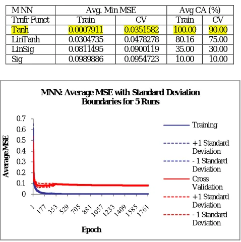
This topology is recommended on the basis of experimental evidences and optimum performance measures.It is observed that the Avg. of min MSE in hidden layer 1 is least on CV dataset for 10 PEs and that in second hidden layer it is the least for 40 PEs.For hidden layer and output layer PEs, different Transfer Functions, such as, Tanh, Sigmoidal, Linear Tanh, Linear Sigmoidal, Softmax, Bias, Linear and Axon and different Learning Rules namely, Standard back propagation algorithm with Step, Momentum, Conjugate Gradient, Quick-propagation and Delta Bar Delta were tested for training and testing the network.Thus, the architecture of MNN shown in Fig. 4 is132-10-40-10. The number of PEs used in the upper module 1 [U1] and that in upper module 2 [U2] is 5 each. Further, lower module 1 [L1] and module 2 [L2] contains 20 PEs each. The analysis of the classification performance shows that the choice of transfer function should be “Tanh” in hidden as well as output layer and the best learning rule is observed as a standard backpropagation algorithm with momentum. Following Fig. 5 shows the variation of average MSE on training as well as CV dataset with respect to number of epochs along with the standard deviation, when the MNN is retrained five times. It is noticed that this error goes on decreasing initially very rapidly and it reduces to the minimum in about 300 epochs.

U1 U2

L1 L2

(7)

I

nternational

J

ournal of

I

nnovative

R

esearch in

C

omputer

and

C

ommunication

E

ngineering

TABLE VI. VARIATION OF TRANSFER FUNCTION OF PES

Fig.5 MNN – Average MSE with Standard Deviation Boundaries for 5 Runs

This MNN network has been trained for different transfer functions of PEs in both the hidden layers and as demonstrated in Table VI, choice of ‘tanh’ transfer function in both the hidden layers resulted into the best classification performance even on CV dataset.

C. PRINCIPAL COMPONENT ANALYSIS (PCA)NN

Principal Component Analysis (PCAs) combines unsupervised and supervised learning in the same topology. Principal component (PC) analysis is an unsupervised linear procedure that finds a set of uncorrelated features, principal components, from the input. A MLP is supervised to perform the nonlinear classification from these components.

The fundamental problem in pattern recognition is defining the data features that are important for the classification (feature extraction). The goal is to transform the input samples into a new space (the feature space) such that the information about the samples is kept, but the dimensionality is reduced. This makes the classification job much easier. Principal component analysis (PCA) is such a technique.

PCA is normally done by analytically solving an Eigenvalue problem of the input correlation matrix. Sanger and Oja demonstrated that PCA can be accomplished by a linear, single layer neural network trained with a modified Hebbian learning rule. Sanger’s rule is recommended, since it orders the projection.

PCA can be used for data compression, producing the M most significant linear features. When usedin conjunction with a multilayer perception (MLP) to perform classification, the [separability] of the classes is not always guaranteed. If the classes are not sufficiently separated, the PCA will extract the largest projections while the separability could be contained within some of the smaller projections.

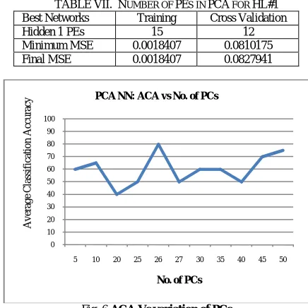
For determination of hidden layer PEs, the procedure that was earlier used in GFFNN is applied. Table VII show that the number of PEs in the first hidden layer should be 12.

The importance of PCA analysis is that the number of inputs for the classifier can be significantly reduced from 132 to 26 PCs. This results in a reduction of the number of required training patterns and a reduction in the training times of the classifier.

0 0.1 0.2 0.3 0.4 0.5 0.6 0.7

A

v

er

a

g

e

M

S

E

Epoch

MNN: Average MSE with Standard Deviation Boundaries for 5 Runs

Training

+ 1 Standard Deviation - 1 Standard Deviation Cross Validation + 1 Standard Deviation - 1 Standard Deviation

M NN Avg. Min MSE Avg CA (%)

Trnfr Funct Train CV Train CV

Tanh 0.0007911 0.0351582 100.00 90.00

LinTanh 0.0304735 0.0478278 80.16 75.00

LinSig 0.0811495 0.0900119 35.00 30.00

(8)

I

nternational

J

ournal of

I

nnovative

R

esearch in

C

omputer

and

C

ommunication

E

ngineering

The architecture of the proposed PCA NN is (Number of Input PCs – Hidden Layer#1 PEs – Output Layer PEs) i.e. 26 PCs-12-10.

The selected parameters for PCA NN are given below:

Number of epochs=1100, Exemplars for Training=34, Exemplars for Cross Validation/Testing=17, Number of Hidden Layer=01, Transfer Function:Tanh, Learning Rule:Momentum.

Fig.6 depicts the variation of the number of PCs with respect to Average Classification Accuracy (ACA). It is found that the ACA is 80% on CV dataset for PCA NN with number of PCs=26.

TABLE VII. NUMBER OF PES IN PCA FOR HL#1

Hidden 1 PEs 15 12

Minimum MSE 0.0018407 0.0810175

Final MSE 0.0018407 0.0827941

Fig. 6 ACA Vs variation of PCs

D. SUPPORT VECTOR MACHINE (SVM)

The Support Vector Machine (SVM) is implemented using the Kernel Adatron algorithm. The Kernel Adatron maps inputs to a high-dimensional feature space, and then optimally separates data into their respective classes by isolating those inputs which fall close to the data boundaries. Therefore, the Kernel Adatron is especially effective in separating sets of data, which share complex boundaries as shown in Fig.7.

0 10 20 30 40 50 60 70 80 90 100

5 10 20 25 26 27 30 35 40 45 50

A

v

er

ag

e

C

la

ss

if

ic

at

io

n

A

cc

u

ra

cy

No. of PCs PCA NN: ACA vs No. of PCs

0.2 0.3 0.4 0.5 0.6 0.7 0.8 0.9 1

0 0.1 0.2 0.3 0.4 0.5 0.6 0.7

En

e

rg

y

H248

Euphorbia geniculata GloriosaSuperba Jasmin brassica nigra

0 0.1 0.2 0.3 0.4 0.5 0.6

1 500 999 1498 1997 2496 2995 3494 3993 4492 4991

A

v

er

a

g

e

M

S

E

SVM: Average MSE with Standard Deviation Boundaries for 5 Runs

Training

+ 1 Standard Deviation

- 1 Standard Deviation

Cross Validation

+ 1 Standard Deviation

(9)

I

nternational

J

ournal of

I

nnovative

R

esearch in

C

omputer

and

C

ommunication

E

ngineering

Website:www.ijircce.com Vol. 5, Issue 1, January 2017

Hence, SVMs are used for classification problem. Fig.8 shows the graph of average Mean Squared Error (MSE) in Training and Cross Validation dataset. Overall Confusion matrix and MSE, NMSE and % classification accuracy for CV dataset with respect to classifiers based on GFFNN, MNN, PCA and SVM have been illustrated in Table VIII and the color scheme for representation of each classifier is portrayed in Table IX.

TABLEVIII. CONFUSION MATRIX AND PERFORMANCE MEASURES OF GFF NN, MNN, PCA AND SVM BASED CLASSIFIER ON CROSS VALIDATION DATASET Output /

Desired Pollen Class

Morinda tomentosa

Madhuca indica

Jatropa panduraefolia

Jasmenium officinale

Impatiens balsamina

Gloriosa superba

Euphorbia geniculata

Erythrina suberosa

Callistemon citrinus

Brassica nigra

Morinda tomentosa

2 1 0 0 0 0 0 0 0 0 0 0 0 0 0 0 0 0 0 0

2 0 0 0 0 0 0 0 0 0 0 0 0 0 0 0 0 0 0 0

Madhuca indica

0 0 1 1 0 0 0 0 0 0 0 0 0 0 0 0 0 0 0 0

0 0 0 0 1 1 0 0 1 0 0 0 0 0 0 0 0 0 0 0

0 0 0 0 1 1 0 0 0 0 0 0 0 0 0 0 0 0 0 0

0 0 0 0 0 0 2 2 0 0 0 0 0 1 0 0 0 0 0 0

0 0 0 0 0 0 2 2 0 0 0 0 1 0 0 0 0 0 0 0

0 1 0 0 0 0 0 0 1 1 0 0 0 0 0 0 0 0 0 0

0 0 0 0 0 0 0 0 2 1 0 0 0 0 0 0 0 0 0 0

0 0 0 0 0 0 0 0 0 1 2 2 0 0 0 0 0 0 0 0

0 1 0 0 0 0 0 0 0 1 2 2 0 1 0 0 0 1 0 2

0 0 0 0 0 0 0 0 0 0 0 0 2 1 0 0 0 0 0 0

0 0 0 0 0 0 0 0 0 0 0 0 1 1 0 0 0 0 0 0

0 0 0 0 0 0 0 0 0 0 0 0 0 0 1 1 0 1 0 0

0 0 0 0 0 0 0 0 0 0 0 0 0 0 1 0 1 1 0 0

0 0 0 0 0 0 0 0 0 0 0 0 0 0 0 0 2 1 0 0

0 1 0 0 0 0 0 0 0 0 0 0 0 0 0 1 1 0 0 0

Brassica nigra

0 0 0 0 0 0 0 0 0 0 0 0 0 0 0 0 0 0 2 2

0 0 0 0 0 0 0 0 0 0 0 0 0 0 0 0 0 0 2 0

Performance Morinda

tomentosa

Madhuca indica

Brassica nigra

MSE 0.03 0.02 0.00 0.02 0.05 0.01 0.01 0.04 0.08 0.11 0.03 0.06 0.01 0.04 0.06 0.04 0.04 0.09 0.00 0.01 0.01 0.12 0.04 0.08 0.01 0.09 0.03 0.09 0.02 0.09 0.04 0.19 0.05 0.13 0.05 0.08 0.05 0.13 0.00 0.17

NMSE 0.31 0.02 0.11 0.44 0.90 0.35 0.14 0.43 0.81 1.13 0.37 0.64 0.17 0.42 1.22 0.90 0.46 0.89 0.07 0.14 0.13 1.18 0.79 1.45 0.35 1.68 0.31 0.95 0.27 0.87 0.45 1.89 0.51 1.31 0.98 1.48 0.48 1.27 0.05 1.64 Percent

Correct 100 50 100 100 100 100 100 100 50 50 100 100 100 50 100 100 100 50 100 100 100 0 100 100 100 100 100 100 100 50 100 100 50 50 100 0 50 0 100 0

TABLE IX: COLORSCHEME FOR DATA REPRESENTATION

GFF NN PCA NN

MNN SVM

TABLEX. PERFORMANCECOMPARISONOFVARIOUSCLASSIFIERSBASEDONNEURALNETWORKS

Neural Network Configuration

MSE NMSE ACA (%)

Training CV Training CV Training CV

GFF NN (132-04-29-10) 0.002385679 0.037154717 0.03413808 0.462615931 100 95

MNN (132-10-40-10) 0.000791181 0.035158250 0.014818069 0.438463430 100 90

PCA NN (26 PCs-12-10) 0.001574631 0.053105406 0.024873298 0.625204834 100 80

(10)

I

nternational

J

ournal of

I

nnovative

R

esearch in

C

omputer

and

C

ommunication

E

ngineering

Following are the typical SEM images of some pollen species along with their appropriate botanical names

Brassicanigra Callistemoncitrinus Erythrinasuberosa Euphorbiageniculata

Gloriosasuperb Impatiensbalsamina Jasmeniumofficinale Jatropapanduraefolia

Madhucaindica Morindatomentose

Fig.9. Typical SEM images of sample pollen species

IV.CONCLUSION

Experimental evidences show that the proposed improved pollen classification method based on neural network work very well. The classification accuracy of GFF NN is found to be reasonable consistently in respect of rigorous testing using training and cross-validation data giving 95% classification accuracy.

The simulated results reveal that computational complexity of the proposed classifier is reduced by using lesser number of connection weights and parameters in the feature dataset. The proposed method is effective, stable and reliable for a pollen classifier with pollen samples from ten different plant species. Even though number of pollen samples in the training data is less (only 34 samples representing 10 different classes), the learning ability of the proposed GFFNN is quite remarkable.

It is seen from Table X, that the GFF NN with architecture 132-04-29-10 clearly outperforms all other classifiers on the basis of results on pollen image classification accuracy.

(11)

I

nternational

J

ournal of

I

nnovative

R

esearch in

C

omputer

and

C

ommunication

E

ngineering

REFERENCES

1. Agashe S. N., Palynology and its applications. pp. 16-48, 2006.

2. Li P.and Flenley J. R., Pollen texture identification using neural networks. Grana, pp. 59-64, 1999.

3. Li P., Treloar W. J., Flenley J. R., Empson L., Towards automation of palynology 2: the use of texture measures and neural network analysis for automated identification of optical images of pollen grains, Journal of Quaternary Science, vol.19, issue 8, pp.755 – 762, Dec.2004.

4. Rodriguez-Damian M., Cernada E., Formella A., Sa-Otero R., Pollen Classification using brightness-based and shape-based descriptors. Proceedings of the 17th_{International Conference on Pattern Recognition ICPR, vol.2, pp.212-215, Aug.2004.}

5. Rodriguez-Damian M., Cernadas E., Formella A., Gonzalez A, Automatic Identification and Classification of Pollen of the Urticaceae Family”,

Proceedings of Acivs (Advance Concepts for Intelligent Vision Systems), Ghent, Belgium, Sept.2-5, 2003.

6. Travieso C.M., Bnceno, J.C., Ticay-Rivas, J.R., Alonso, J. B., “Pollen classification based on contour features”, 15th International Conference on Intelligent Engineering Systems (INES, pp.17-21), Jun 2011.

7. Carrion P., Cernadas E., Sa-Otero P., Diaz-Losada E., Improved classification of pollen texture images using SVM and MLP.

8. Nguyen N. R., Donalson-Matasci M., Shin M. C., Improving pollen classification with less training effort, IEEE Workshop on Applications of

Computer Vision (WACV), Tampa, FL, pp.421 – 426, 2013.

9. Kalva P. R., Curitiba Enembreck F., Koerich A. L., Web Image Classification using Classifier Combination. IEEE Latin America Transactions,

vol.6, Issue 7,pp. 661 – 671,Dec. 2008.

10. Hidalgo M. I. and Bootello M/ L., About some physical characteristics of the pollen loads collected by Apis mellifera L. Apicoltura, 6:179-191, 1990.

11. Dhawale V. R., Tidke J. A., Dudul S. V., Neural Network Based Classification of Pollen Grains. IEEE Publication on International Conference

on Advances in Computing, Communications and Informatics (ICACCI), pp.79-84, 2013.

12. Sa´-Otero, M. P. de, Gonza´ lez, A. P., Rodrı´guez-Damia´n, M. and Cernadas, E, Computer-aided identification of allergenic species of Urticaceae pollen. – Grana 43: 224–230. ISSN 0017-3134, 2004.

13. Langford M., Taylor G. E., Flenley J. R., Computerized identification of pollen grains by texture analysis, Elsevier B.V. Review of Palaeobotony and Palynology, vol. 64, Issues 1-4, pp. 197-203, Oct.1990

14. Holt K., Allen G., Hodgson R., Marsland S., Flenley J., Progress towards an automated trainable pollen location and classifier system for use in the palynology laboratory. Review of Palaeobotany and Palynology, Vol. 167, Issues 3-4, pp. 175-183, Oct. 2011.

15. Haykin S., Neural Networks. Prentice-Hall, 1999.

16. Cortes C. and Vapnik V., Support Vector Networks. Machine Learning, (20): 273-297, 1995.

BIOGRAPHY

V.R. Dhawaleis Assistant Professor and Head, Department of MCA, Vidya Bharati Mahavidyalaya, Amravati, Maharashtra. He received Doctorate degree in 2015 from SGBAU, Amravati, MS, India. His research interests are Computational Intelligence, Artificial Intelligence, and Algorithms etc.

J.A. Tidke (Former-Pro-Vice Chancellor, SGBAU,Amravati) is a Professor and Head, Department of Botany, Sant Gadge Baba Amravati University, Amravati, Maharashtra. He received Doctorate degree in 1999 from SGBAU, Amravati, MS, India. He has done Post-doctoral Fellowship at Laboratory of Pollination Ecology, Institute of Evolution, Haifa University, Haifa (Israel). His research interests are Aeropalynological studiesandPaleobotany, etc.