Efficient skycube computation using bitmaps

(1)

Efficient SKYCUBE Computation using Bitmaps

derived from Indexes

Gayathri Tambaram Kailasam

North Carolina State University

Jaewoo Kang

North Carolina State University

Abstract

Skyline queries have been increasingly used in multi-criteria decision making and data mining applications. They retrieve a set of interesting points from a potentially large set of data points. A point is said to be interesting if it is as good or better in all dimensions and better in at least one dimension. Skyline Cube (Skycube) consists of skylines of all possible non-empty subsets of a given set of dimensions. In this paper, we propose two algorithms for computing skycube using bitmaps that are derivable from indexes. Point-based skycube algorithm is an improvement over the existing Bitmap algorithm, extended to compute skycube. Point-based algorithm processes one point at a time to check for skylines in all subspaces. Value-based skycube algorithm views points as value combinations and probes entire search space for potential skyline points. It significantly reduces bitmap access for low cardinality di-mensions. Our experimental study shows that the two al-gorithms strictly dominate, or atleast comparable to, the current skycube algorithm in most of the cases, suggesting that such an approach could be an useful addition to the set of skyline query processing techniques.

1. Introduction

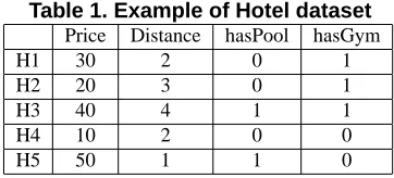
Skyline queries are increasingly used in decision support applications such as multi-criteria decision making, data mining, visualization [1] and user-preference queries. A Skyline query overddimensions returns a set of points that are not dominated by any other point in those dimensions. A point dominates another point if it is as good or better in all dimensions and better in at least one dimension. Con-sider an example scenario where a person travels to a city and wants to select a hotel to stay by searching the database of hotels in the city. An example dataset is shown in Table 1.

A user who is particular about hotel facilities may issue a skyline query to search for hotels that are close to beach,

Table 1. Example of Hotel dataset Price Distance hasPool hasGym

H1 30 2 0 1

H2 20 3 0 1

H3 40 4 1 1

H4 10 2 0 0

H5 50 1 1 0

has pool and gym facilities. The result of this query will include H5, H1 and H3. These hotels are not dominated by other hotels and hence will be interesting to the user. H2 is dominated by H1 as H1 is closer to the beach than H2 and also has gym facilities. Similarly, H4 is dominated by H1 as H1 has gym facilities in addition to being at the same dis-tance from beach as compared to H4. By eliminating hotels that are completely dominated, decision making process can be made much easier for the user.

The same dataset, shown in Table 1 may also be subject to other skyline queries. For example, some customers may prefer cheap hotels that are close to beach. They will issue a skyline query for Price and Distance dimensions. While some others who intend to stay in hotel for a longer period may prefer cheap hotels with excellent facilities and hence may require skyline of Price, hasPool and hasGym dimen-sions. Depending on the customer preferences, one may ex-pect a skyline query for any subset of dimensions included in the dataset. This is especially true in decision support systems where every parameter is likely to be of interest to some set of users. Algorithms that efficiently calculate Sky-cube (skyline results for all possible dimension subsets) can be very useful for such applications.

(2)

point is skyline in any dimension subset. Both the algo-rithms are completely non-blocking and hence have very low response times.

The first algorithm, called Point-based skycube, is an im-provement over the single skyline Bitmap algorithm [11] extended to calculate Skycube. In this approach, each record is mapped to an m-bit vector, where m is the sum of the number of distinct values in all dimensions. Once the bitmaps are pre-computed, the algorithm steps through each point to check if it belongs to skyline of any subset of dimensions. It also identifies the duplicates of the current point and masks the points that are dominated by the current point. By identifying duplicates and dominated points (not done in original Bitmap algorithm), the number of points to be processed by the algorithm are significantly reduced.

The second algorithm, called Value-based Skycube searches the dimensions for prospective skyline points start-ing with highest value in all dimensions and steppstart-ing down each time the value combination is invalid (no point ex-ists corresponding to the value combination). Once a sky-line point is identified, all the value combinations below it are pruned as they are guaranteed to be dominated by the current value combination. The algorithm then repeats the process with next non-dominated value combination. This algorithm is optimized for dimensions with low cardinality where the search space of every value combination of all dimensions is much less than the search space of all points in the database.

Skycube results are typically materialized for faster re-trieval. But in some applications where this is not pre-ferred, especially when data is prone to updates, it would be beneficial to materialize some update-friendly interme-diate results as this would return results faster than querying base data. Our skycube algorithms are very much applica-ble in these scenarios. By materializing the bitmaps, which are easily updatable, skycube results can be obtained much faster. This has an added advantage while servicing user-preference queries.

For example, suppose that the user has a preference for a particular set of hotels and would like to know if any of those hotels are a part of final skyline or if there are any ho-tels that are better than the current choices. While existing algorithms may have to run to completion before they could publish the results, which may take significant amount of time, our Point-based algorithm only needs to access the bitmaps corresponding to the selected hotels to return the results. Another example is where the user enters a range skyline query as follows: return the list of skyline hotels with price: 10-30, distance: 2-4 and hasGym. Instead of computing the entire skyline and then filtering the results, the Value-based algorithm can be made to run only for the specified range of values and hence resulting in very low response time. This is especially attractive because datasets

used for decision support systems tend to be very large and calculating skycube and then applying the user filter may turn out to be very expensive.

The rest of the paper is organized as follows. In the next section we survey various skyline algorithms proposed in the literature. In Section 3, we explain the Single sky-line Bitmap algorithm, which forms the basis for our Point-based algorithm. Section 4 explains how bitmaps can be calculated from database indexes. Sections 5 and 6 ex-plain the Point-based and Value-based skycube algorithms respectively. We provide a thorough experimental evalua-tion in Secevalua-tion 7 and finally conclude in Secevalua-tion 8.

2. Related Work

This section explains briefly the existing single skyline and skyline subspace algorithms. For the rest of the paper, we shall be considering skylines only for MAX annotations (preferring points with high values in all dimensions) [1], without any loss of generality.

The skyline operator was first introduced by Borzsonyi et al. in [1]. The paper was the first to propose skyline al-gorithms in database context namely, block nested loops, divide and conquer and B-tree based algorithms. Block Nested Loop (BNL) compares each point with every other point efficiently by keeping a self-organizing list of candi-date skyline points in memory. Chomicki et al. proposed an improvement over BNL algorithm by first sorting the dataset according to a monotone sorting function [2]. Di-vide and Conquer (D&C) algorithm diDi-vides the dataset into several partitions, calculates skylines within partitions using a main memory algorithm and merges the result to output the final skyline points. A new D&C algorithm for comput-ing 2D skylines with optimal I/O costs was proposed by Lu et al. in [7].

Tan et al. were the first to propose progressive skyline algorithms based on bitmaps and indexes [11, 3]. Bitmap algorithm is explained in detail in the next section. Index al-gorithm transforms the points into single dimensional space and organizes them into disjoint lists, each indexed using a B-tree to return skyline points in batches. Nearest Neighbor (NN) was another progressive (online) algorithm proposed by Kossmann et al. in [6]. NN algorithm applies the divide and conquer framework on datasets indexed by R-trees and uses nearest neighbor search techniques [4, 10]. Branch and Bound skyline (BBS) algorithm was proposed in [8] as a progressive and I/O optimal algorithm. It efficiently prunes points by accessing only those R-tree nodes that may con-tain skyline points.

(3)

might exponentially increase the number of structures that need to be built on the dataset or 2) are not optimized for calculating skycube as do not adopt any resource or compu-tation sharing strategies.

Recently, lot of research has been going on in the area of skyline subspaces. Yuan et al. were the first to propose al-gorithms to efficiently compute skycube [13] which consists of skylines of all possible dimension subspaces. Bottom-Up Skycube (BUS) computes skycube in a level-wise, bottom up manner. Each skyline computation uses the results and sorting output of the level below it. The Top-Down Skycube (TDS) extends the basic Divide-and-Conquer algorithm by computing multiple related skyline queries simultaneously. BUS or TDS algorithm adopts several result and computa-tion sharing strategies, while our algorithms reuse the in-dexes built on the dimensions in addition to sharing compu-tation and bitmap accesses.

Pei et al. introduced the notion of skyline groups and de-cisive subspaces in [9] and proposed an algorithm, Skyey, to compute subspace skyline points. Tao et al. proposed the SUBSKY algorithm in [12] to efficiently support sky-line queries in any subspace. This differs from the skycube algorithms in that SUBSKY aims at computing the skyline of one particular subspace as opposed to all subspaces.

3. Bitmap Algorithm for computing Skylines

This algorithm [11] uses a customized bitmap structure to store all the information required to calculate the sky-line points. For example, suppose that we haved dimen-sional dataset consisting of D points. Each point x = (x1, x2, ..., xd)in the dataset is encoded into an m-bit

vec-tor, where m is the total number of distinct values across all dimensions.

• Letki be the number of distinct values for dimension

i,1 <= i <= d. Then m = Pd_i₌₁ki. Let pij be

thejth _{distinct value in dimension}_i _{and each}_p ij >

pij+1. Then eachpij is represented byki bits where

most significant1toj−1bits are set to 0 and the rest of the bits are set to 1.

• Eachxi must be equal to somepij and is mapped to

thatpij’s bit vector of lengthki.

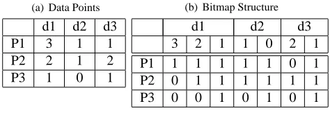
Consider an example shown in Table 1(a). The 3-dimensional dataset consists of 3 points. Each of the dimen-sions have 3, 2 and 2 distinct values and hence every point is mapped to a 7{3+2+2}bit vector as shown. Consider second pointP2{2,1,2}. The point has 2nd largest value in dimension d1. Hence it is mapped to bitvector 011. Simi-arly it has highest value in 2nd dimension (11), and highest value in third dimension as well(11). Hence the bitmap cor-respoding toP2{2,1,2}={011,11,11}

(a) Data Points

d1 d2 d3

P1 3 1 1

P2 2 1 2

P3 1 0 1

(b) Bitmap Structure

d1 d2 d3

3 2 1 1 0 2 1

P1 1 1 1 1 1 0 1

P2 0 1 1 1 1 1 1

P3 0 0 1 0 1 0 1

Table 2. Example 1

LetBSijdenote the bit-slice for thejthdistinct value of

the ithdimension. It corresponds to the column vector in

Table 1(b). Number of bits inBSijwill be equal toD, total

number of tuples in dataset. A bit that is set in positionk will indicate that recordP k has a value ofj or higher in dimension i. In our example, BS13 = 100. This bitmap

indicates the records that have a value of 3 or higher in d1 dimension. In our dataset, onlyP1has a value≥3 in d1. Hence the bitmap has 1 forP1, 0 forP2and 0 forP3.

To check if a pointx= (x1, x2, ..., xd)is in the skyline,

the following bitmap operations need to be performed:

1. LetA= Bitwise-and of the bit slices corresponding to valuesx1,x2, .. xd. A bit that is set in positioniof

the resulting bitmap means that recordP ihas values that are good or better than the current point,x, in all dimensions.

2. LetB = Bitwise-or of the bit slices corresponding to just one value higher than each ofx1,x2, .. xd. A bit

that is set in positioniof the resulting bitmap indicates that recordPihas higher value than current point,x, in

at least one dimension.

3. LetC= Bitwise-and of results [1] and [2]. A 1 in posi-tioniof the resulting bitmap means that recordP ihas value that is as good or better thanxin all dimensions and better in at least one dimension when compared tox. In other words,Pi dominatesx. If on the other

hand, the resulting bitmap is all 0’s, then no point dom-inatesxand hencexis a skyline point.

Example 1: Referring to the dataset in Table 2, to

determine if pointP2(2,1,2)is in the skyline of all three dimensions, we carry out the above operations:

A= 110&110&010 = 010

This indicates that no point (other than P2 itself) has values that are good or better thanP2in all dimensions.

B= 100|000|000 = 100

(4)

C=A&B= 010&100 = 000

This indicates there is no point that has equal or higher value thanP2in all dimensions and strictly higher value in at least one dimension. HenceP2is a skyline point.

3.1. Applicability of Bitmap Algorithm for Skycube

computation

There are certain characteristics of the bitmap algorithm that make it very suitable for Skycube computation.

• Bitmap Reuse: One of the major limiations of the bitmap algorithm is the cost of accessing the bitmaps. For each point, 2 ×d bitmaps have to be accessed wheredis the number of dimensions (dfor calculat-ingAvalue and anotherdaccesses for calculatingB value). It is worthwhile to note that the bitmaps ac-cessed to check if pointP is in skyline for a particular dimension set can be easily reused for checking if the point is skyline in any of its subsets. This reuse of bitmap amortizes their access cost over the computa-tion of skylines for all non-emtpy dimension subsets and hence could lead to better performance.

• Computation Reuse: On the lines of the above argue-ment, if the same set of bitmaps could be used, then the bitwise-and and bitwise-or of those bitmaps can be reused as well.

From above, we can clearly see that the cost of bitmap access for computing single d-dimensional skyline using bitmap approach is same as the cost of bitmap access for computing skycube for all non-empty dimension subsets (2d₋_{1). We now turn to explain our algorithms for}

com-puting skycube using the bitmap structure.

4. Using Indexes to build Bitmap structure

This section explains how to compute bitmaps from data-base indexes. The bitmap structure computed as explained in the previous section gives information about records that have a value greater than or equal to the current point’s value in a specific dimension. This information can be eas-ily extracted from the database indexes, if we assume we have either a Bitmap index or B+ tree index on each of the columns included for skycube computation.

• Bitmap Index on a particular dimension maintains a bitmap for each distinct value present in the dimen-sion. Each bit in the bitmap corresponds to a record, and if the bit is set, it means that the record contains the key value. The bitmap structure used in Bitmap skyline algorithm can be built from Bitmap index by doing a Bitwise-OR of bitmaps of all values greather than and

including the current value. The resulting bitmaps will have the bits set for all records that have values greater or equal to the key value. Hence by just doing one pass over the bitmap index, the bit structure in Table 1(b) can be easily computed.

• B+ Tree Index can also be used to build the bitmap structure in Table 1(b). By scanning the leaf pages of the index from the greatest to the smallest order, one will be able to retrieve the sorted order of the records for the dimension on which the index is built. Once we have a sorted list, building the bitmap structure for that dimension is straightforward.

Many single skyline algorithms require a specific struc-ture, either in R-tree or B+-tree format, for a particular set of dimensions. The disadvantage with this is that these struc-tures are special purpose data strucstruc-tures only used in skyline computation and have very little use outside of skyline ap-plications. Whereas, in a typical decision support system, if any dimension is important enough to be included in sky-cube computation it is reasonable to assume either B+ tree or Bitmap index to exist on that dimension since they might be needed by lots of other applications as well. Note that even in the absence of the index for some or all dimensions, the bitmap structure can still be computed by sorting the dataset on the non-indexed dimensions. Database indexes are usually optimized for disk acess and would give bet-ter performance than any user implemented structures. The bitmap structure can either be pre-computed or computed on the fly.

5. Point-based Skycube Algorithm

Despite the simplicity of the bitmap algorithm presented in Section 3, it has some serious limitations:

• The bit operations have to be performed for every point in the dataset. This could be prohibitively expensive for large datasets. By applying some efficient prun-ing techniques, many points can be ruled out without accessing their bitmaps.

• The algorithm fails to retrieve the maximum possible information from the bitmap. For example, the algo-rithm accesses the same set of bitmaps for every dupli-cate record found in the dataset. If the algorithm were able to identify duplicates, these extra bitmap accesses and subsequent bit operations can be avoided, thus sig-nificantly reducing the runtime of the algorithm.

(5)

aims to retrieve the maximum possible information from the bitmap by identifying points that are duplicate of and dom-inated by the current point. We also propose an heuristic technique to process the points having maximum dominat-ing power first. The followdominat-ing sections explain the steps in detail.

5.1. Point Pruning Techniques

5.1.1 Pruning Duplicate Points

The bit slices accessed by a particular record are determined by the values that the record holds in a particular dimen-sion. Hence every point that has the same value in all or some of the dimensions, will repeatedly access the same set of bitmaps and thereby increasing the number of bitmap accesses. It should also be noted that, if a point is not in the skyline for a particular set of dimensions, then none of its duplicates are skyline points as well and vice versa. By identifying and eliminating duplicates, we not only reduce bitmap access but also converge to result faster as the total number of points that need to be processed by the algorithm are significantly reduced.

Recall the computation ofAandCvalues from Section 3. Abitmap has bit set for those records that have a value higher or equal to the corresponding dimension values in the current record andCbitmap has bit set for records that dominate the current record. The difference (bitwise-xor) between the two bitmaps identifies the records that have the same value as the current record in all the dimensions:

duplicates=AxorC.

Hence by applying the result of current record to all its du-plicates, we can avoid processing them separately.

5.1.2 Pruning Dominated Records

For each point in the dataset, the original bitmap algorithm only checks if the current point is dominated by some other point. It would be beneficial to identify and prune points dominated by the current point as well. This can easily be done without any extra computation or extra bit access.

Recall that theB value computed in the bitmap algo-rithm has bit set for those points that have a value greater than the current point in at least one dimension. That means if a bit is not set for a particular point, then all of its values are either equal or lesser than the current point. In other words, these points are either duplicates of current point in all dimensions or dominated by current point. Since dupli-cates are handled separately as mentioned above, the points that have bits unset in B bitmap can be pruned from further processing.

5.2. Point-based Skyline Cube Algorithm

The algorithm, listed in Algorithm 1, maintains a Mask (or pruned) bitmap of lengthD(number of tuples) for every non-empty dimension subset. The bitmaps indicate records that are masked from processing in each of the dimension subsets. The bitmaps are initialized to 1, indicating that no points are pruned in the beginning. The algorithm first cal-culates all single dimensional skylines. Since, these points have a high value in at least one dimension and are less likely to be dominated by other points, they are the first points to be considered for calculating Skyline cube (shown in Algorithm 2).

Algorithm 1 Point-based Skyline Cube

1: for each non-empty dimension subsetido

2: initialize the mask bits to 1

3: end for

4: for1≤j≤d do

5: List L = Points with maximum value in this dimen-sion

6: for each point P in L do

7: CheckSkylineCube(P)

8: end for

9: clear the mask bits to 0 indicating that the current dimension is completed

10: end for

11: while (List L = getNextPoints()) is not empty do

12: for each point P in L do

13: CheckSkylineCube(P)

14: end for

15: end while

After calculating one-dimensional skylines (lines 4-10), the algorithm retrieves the next batch of points to be processed and checks each point for skyline in all dimen-sion subsets (lines 12-14).

Algorithm 2 CheckSkylineCube(Point P)

1: for each non-empty non-single dimension subset of P

do

2: if P is not masked in this dimension subset then

3: check if P is skyline point

4: apply the result to duplicates of P

5: mask the points dominated by P for this dimension set in addition to masking P and its duplicates

6: end if

7: end for

(6)

al-gorithm. If a point with high dominating power is processed first, it would prune out more number of points earlier, lead-ing to potentially less number of steps to completion. In or-der to improve the performance, we propose the following heuristic approach for this ordering:

• The points with maximum dominating power are less likely to be masked in many dimension subsets. Also more points would be masked at lower levels of the lattice (e.g. 1 dimension) than at the upper levels (e.g. d dimensions). Hence, one heuristic technique to re-trieve the next batch of points would be to do a bitwise-& of mask bitmaps starting at top level of the lattice, going down one level at a time and stopping just be-fore all points are masked. The points that are still unmasked in this step will be included in the batch for next processing. We have used this technique in our implementation.

6. Value-based Skyline Cube Algorithm

It is quite obvious that since Point-based algorithm processes a single point at a time, the same bit slices may be accessed multiple times. They do not have any specific access pattern and hence caches might not be of much help. As a result, the performance of Point-based algorithm de-grades rapidly as the size of the dataset grows (i.e. the number of points to process increases). Consider a case where each dimension has a small number of distinct val-ues and the dataset contains 1 million points. If there are more dimensions, there will be lot more skyline points and the Point-based algorithm might take significantly long time to converge. In order to optimize the bit access, we pro-pose the Value-based Skyline algorithm which exhaustively searches the value combinations for potential skyline points instead of enumerating the points.

6.1. Bitmap Structure for Value-based Algorithm

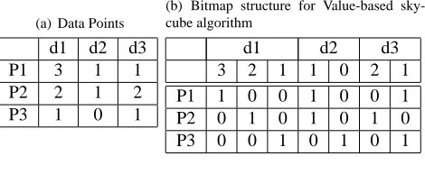
There is a slight difference in way the bitmaps are calcu-lated for Value-based algorithm. For Point-based skycube algorithm, ifpijis thejthdistinct value in dimensioniand

eachpij > pi(j+1), then eachpijwas represented bykibits

where most significant1 toj−1bits are set to 0 and the rest of the bits are set to 1.

For Value-based algorithm, ifpijis thejthdistinct value

in dimensioni, then onlyjthbit ofpij will be set to 1. Rest

of the bits will be set to zero. Table 3 shows the bitmap used by Value-based algorithm for our example dataset.

It is quite clear from the table that the bitmap structure required by Value-based algorithm is no different from the conventional bitmap index on each of the dimensions. It means that for the dimensions having bitmap indexes, no

(a) Data Points

d1 d2 d3

P1 3 1 1

P2 2 1 2

P3 1 0 1

(b) Bitmap structure for Value-based sky-cube algorithm

d1 d2 d3

3 2 1 1 0 2 1

P1 1 0 0 1 0 0 1

P2 0 1 0 1 0 1 0

P3 0 0 1 0 1 0 1

Table 3. Example 2

other extra data structure would be needed. This is one of the main strengths of this algorithm.

6.2. Value-based Skyline Cube Algorithm

The Value-based algorithm, shown in Algorithm 3, starts with highest value combination. For every value combina-tion, it checks if there exists any point corresponding to the current value combination and if there is, the current val-ues are checked for skyline in all dimension subsets. Else, the algorithm retrieves the next interesting point and contin-ues the process until all value combinations are extracted. checkSkyline() method is the same as explained in Algo-rithm 2. The procedure for retrieving the next interesting point, nextValueExists(), is explained in the following sec-tion.

Algorithm 3 Value-based Skyline Cube

1: fori= 1toN U M DIMdo

2: // initial value combination to be checked should be

3: // the combination with maximum values in all

4: // dimensions (has maximum dominating power)

5: values[i] = maxValue[i]

6: end for

7: repeat

8: // isValid returns the first dimension where the value

9: // combination becomes invalid; returns -1 for valid

10: // combinations

11: if (dimToChange = isValid(values)) == -1 then

12: checkSkyline(values)

13: end if

14: until nextValueExists(dimToChange, values)

Before we delve into the details of the algorithm, we want to review the following examples in order to get some insights.

Example 2: In this example, we explain Value-based

skycube algorithm using the dataset shown in Table 2(b).

(7)

the highest value in d1 dimension and 1, 2 are highest values in d2 and d3 dimensions respectively.

2. The algorithm then checks if this value combination is valid. This is done by doing a bitwise-& of the bit slices corresponding to the dimension values. If the resulting bitmap is all zeros, then there does not exist any point with this value combination. Hence the value combination becomes invalid. In our case,

bitwise-& of the bit slices = 100&110&010 = 000 =⇒the value combination is invalid.

3. For invalid points, the next logically lower value has to be tried. This is retrieved by lowering the value in the rightmost dimension, if possible, and increas-ing the value in all subsequent dimensions (if any) to the highest possible value. The next value in our case : (3, 1, 2↓)⇒(3, 1, 1)

bitwise-& of the bit slices = 100&110&101 = 100 =⇒The value combination corresponds to point P1 in our dataset.

4. Once the valid value combination is retrieved, check if the value combination is in skyline of any of dimension subsets. In our example (3, 1, 1) is in the skyline of

{d1},{d1, d2},{d1, d3}and{d1, d2, d3}.

5. Since the value combination was a skyline in{d1, d2, d3}, the next logical value (3, 1, <1) is known to be dominated by the current combination. Hence the al-gorithm does not consider any points in the pruned space (3, 1,<1). There are no such pruned points in this case.

6. For valid points, the next value combination is got by going to the highest value in the rightmost dimension and going to lower value in the dimension preceding to it. i.e. (3, 1↓, 1↑). This ensures that the next value combination is not in the pruned region. In our exam-ples, our next value would be (3, 0, 2). The algorithm then continues the process from step [2] until the entire search space is exhausted.

6.2.1 Retrieving next value combination

This algorithm has two cases: current value combination is either 1) valid value combination or 2) invalid value combi-nation.

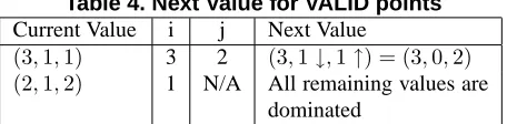
1. Valid value combination: Let’s say the current

valid value combination corresponds to values (x1, x2, ..., xd). The procedure to retrieve the next

in-teresting point does not depend on whether the value combination corresponds to a d-dimensional skyline point or not. This is because, if the current point is

in skyline, then all values combination in the region (x1, x2, ..., < xd)would be dominated by the current

point and hence need not be considered. If the current point is not in the skyline, the current value combina-tion(x1, x2, ..., xd)is itself dominated and hence any

point in the region(x1, x2, ..., < xd)is guaranteed to

be dominated as well.

The next value combination to be considered is obtained by finding the first i for which xi 6=

maxV alue(i)1_,_i ₌ _d_→ _{1. If}_∃_i_{, then update}_x

i =

maxV alue(i). The algorithm then tries to find the first

jfor whichxj 6=minV alue(j)2,j =i−1 →1. If ∃j, then updatexj=next lower value ofxj in

dimen-sion j. If no suchi or j exists, then all value com-binations have been exhausted or dominated and the algorithm is done. Table 4 shows some examples for the same dataset shown in Table 2(a).

Table 4. Next Value for VALID points Current Value i j Next Value

(3,1,1) 3 2 (3,1↓,1↑) = (3,0,2) (2,1,2) 1 N/A All remaining values are

dominated

2. Invalid value combination: Let’s say the current value combination becomes invalid at dimension t. This means that there exists some points with val-ues (x1, x2, .., xt−1) upto t −1 dimensions but no

point matches(x1, x2, .., xt−1, xt)combination in

di-mension t. The next value combination to be con-sidered is obtained by finding the first i for which

xi 6= minV alue(i), starting from i = t → 1.

Up-datexi to the next lower value ofxi in dimensioni.

Then∀j = i+ 1 → d, xj = maxV alue(j). If no

such i exists, then all value combinations have been exhausted and the algorithm is done. Table 5 shows some examples for the same dataset shown in Table 2(a).

Table 5. Next Value for INVALID points Current Value t i Next Value

(3,1,2) 3 3 (3,1,2↓) = (3,1,1) (3,0,2) 2 3 (3↓,0↑,2↑) = (2,1,2)

6.2.2 Dealing with columns having high Cardinality

Since the Value-based algorithm exhaustively searches the entire data space for potential skyline points, it performs

(8)

very well for low number of dimensions and low number of distinct values per dimension. However, it is not uncommon to have some columns with large number of distinct values. In the hotel example shown in Table 1, Price is one such attribute. In a dataset of around 1 million points, the number of distinct price values would be at least 1000. And this increase in number of distinct values in just one dimension could blow up the size of the search space for the Value-based algorithm.

To overcome that, we propose a bucketized version of the Value-based algorithm, where dimensions with high cardi-nality, will be split into multiple levels, each level contain-ing a specified number of buckets. The number of buckets will basically be the number of distinct values at each level. While this increases the dimensionality of the dataset as a result of splitting single dimension into multiple levels, the advantage here is that we only need to access lower levels to compare records within the same bucket. With the interest of space, we omit the details of this generalization. Please refer to [5] for full details.

7. Experimental Evaluation

This section provides a thorough performance analysis of our Point-based and Value-based skycube algorithms. In this section in order to validate our algorithms, we compare the performance of our Point-based and Value-based algo-rithms with the Top-Down skycube (TDS) algorithm pro-posed in [13]. TDS performs much better than Bottom-Up skycube (BUS) algorithms in almost all cases as shown in [13] and hence we do not consider BUS in our experiments. As mentioned before, single skyline algorithms are not op-timized to share computation across dimension subspaces and do not perform well for calculating skycube. As a re-sult we limit our performance evaluation only to the previ-ous skycube algorithm.

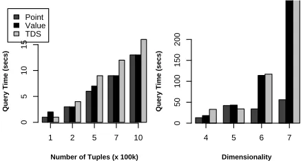
All experiments were carried out on a Linux machine having two Intel Xeon 2.80GHz processors with total 4GB main memory. The algorithms were implemented in C++. Following the common practice in the literature, we used independent, correlated and anti-correlated databases pro-posed in [1] as benchmark databases. We experimented with datasets having cardinality in the range of [100k, 1M] and dimensionality(DIM) in the range of [3,7]. Number of distinct values per dimension, in other words Column Car-dinality (CC), is another important parameter in our exper-iments as it determines the size of the bitmap table. The datasets we used for the experiments have column cardinal-ity in the range of [20, 100]. We measure the query time for the different algorithms for skycube computation. The run time measured for our algorithms include the time taken to build the bitmap structure and the time to compute the sky-cube results.

1 2 5 7 10

Number of Tuples (x 100k)

Query Time (secs)

0

5

10

15

Point Value TDS

(a) Varying Number of Tuples (DIM=4, CC=30)

4 5 6 7

Dimensionality

0

50

100

150

200

(b) Varying Dimensions (# of tu-ples=1M, CC=30)

Figure 1. Point vs. Value vs. TDS for corre-lated dataset

7.1 Comparing Point and Value algorithms

Throughout the experiments, we observed that Value-based algorithm generally outperforms the Point-Value-based counterpart. Only exception was the case with correlated datasets. As shown in Figure 1, with correlated dataset, the Point algorithm outperformed the Value algorithm (and TDS) moderately in varying number of tuples test (Figure 1(a)) and somewhat significantly in varying dimensions test (Figure 1(b)). In the test with varying column cardinality (graph not shown), the point algorithm performed compara-bly with the other two algorithms.

It is because the Point-based algorithm processes points in single dimensional skyline first, most points get pruned in the initial stages of the algorithm as single dimension skyline points are good in other dimensions as well (due to correlated effect). On the other hand, Point algorithm has to process much more points for independent and anti-correlated datasets and hence its performance substantially degrades in those cases. For example, in independent dataset containing 1M points having 4 dimensions and 20 distinct values per dimension, Point algorithm takes 872 seconds to calculate skycube whereas Value and TDS fin-ish in 11 and 30 seconds respectively. Hence, for the rest of our evaluation, we only consider Value and TDS algorithms for independent and anti-correlated datasets.

7.2 Effect of Tuple Cardinality

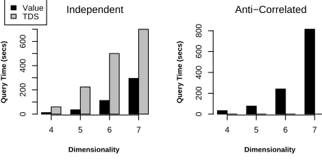
In this experiment, we study the effect of increase in the number of tuples on the overall skycube computation time. We compare the time taken for independent and anti-correlated benchmarks with cardinality between 100k to 1M for 4 dimensions, each dimension having 30 distinct values. Figure 2 shows the results of the experiment.

(9)

1 2 5 7 10

0

5

10

20

Independent Value

TDS

1 2 5 7 10

0

20

60

100

Anti−Correlated

Figure 2. Effect of Cardinality (DIM=4, CC=30)

completely outperforms TDS algorithm in both datasets. Our Value-based algorithm is faster by at least by a fac-tor of 2 for independent datasets and at least by a facfac-tor of 3 for anti-correlated datasets. It should be noted that for Value-based algorithm increase in the number of tuples in-creases the skycube computation time only slightly for both independent and anti-correlated databases, while there is a significant increase in computation time for TDS algorithm. As we can see in Section 7.4, time taken for the Value algo-rithm depends more on the column cardinality than on the number of tuples for a fixed dimension dataset.

7.3. Effect of Dimensionality

To study the effect of dimensionality on our algorithms, we use datasets having 1M tuples, 30 distinct values per di-mension and vary the didi-mensions from 4 to 7. Experimental results are shown in Figure 3.

4 5 6 7

Dimensionality

0

200

400

600

Independent Value

TDS

4 5 6 7

Dimensionality

0

200

400

600

800

Anti−Correlated

Figure 3. Effect of Dimensionality (# of tu-ples=1M, CC=30)[Note: TDS algorithm failed to com-plete for anti-correlated dataset]

It is quite clear from the figure that Value-based algo-rithm is more than 4 times faster than TDS algoalgo-rithm for in-dependent dataset on an average. For example, in 6 dimen-sions, Value algorithm completes in 112 seconds whereas TDS takes 500 seconds to run to completion. Note that

the TDS algorithm failed to compute the skycube for anti-correlated dataset and only the value algorithm is shown in the second graph3_.

7.4. Effect of Column Cardinality

20 30 40 50 70 100

Column Cardinality

0

10

20

30

40

50

Independent

Value TDS

20 30 40 50 70 100

Column Cardinality

0

50

100

150

Anti−Correlated

Figure 4. Effect of Colum Cardinality (# of tu-ples=1M, DIM=4)

Since the size of the bitmap table and hence the perfor-mance of our Value-based algorithm depend on the number of distinct values in each dimension, we study the effect of Column Cardinality on our algorithms. We considered column cardinalities in the range of [20, 100] for a dataset having 1M records and 4 dimensions. Experimental results are shown in Figure 4.

For varying dimensions, our Value-based algorithm is faster on an average by a factor of 2.1 for independent datasets and by a factor of 2.7 on an average for anti-correlated datasets. As the number of distinct values in-creases, search space for Value-based algorithm widens and this explains the increase in computation time. Since TDS algorithm does not depend on the column cardinality, we can expect a break even point before which Value-based al-gorithm would perform better and after which TDS would be preferable to our Value algorithm. In the experiment above, the break even point occurs at column cardinality of 100 for anti-correlated dataset as can be seen from the figure.

7.5. Effect of Point Pruning Strategies

In this section, we study the effect of point pruning strategies on our algorithms. We evaluated the number of bitmap accesses for the original single skyline Bitmap al-gorithm (explained in Section 3) and our Point-based and Value-based algorithms. The experimental results in this section are implementation independent as we measure only

3_{We only obtained the executable from the authors and were not able}

(10)

1 2 5 7 10

No of Tuples (x100k)

# of Bit Access

1 e+02

1 e+05

Independent

Bitmap Point Value

1 2 5 7 10

No of Tuples (x100k)

# of Bit Access

5 e+02

5 e+04

Correlated

Figure 5. Efficiency of Point Pruning Strate-gies(DIM=4, CC=30)[Note: Graph in LOG scale]

the number of bitmap accesses and not the time taken to ac-cess them. It is important to note here that the number of bitmaps accessed by Point/Value based algorithm for cal-culating ddimensional skycube is same as the number of bitmap accesses done for computing single skyline ofd di-mensions. The bitmap accesses were measured for a dataset containing 1M records and 4 dimensions.

Results shown in Figure 5 explain the efficiency of our pruning strategies. We show the results only for indepen-dent and correlated datasets as the trend for anti-correlated dataset was very similar to independent dataset. It can be clearly seen that our skycube algorithms are orders of mag-nitude better than the original Bitmap algorithm. Also, as explained above, Point algorithm performs better for cor-related datasets whereas Value algorithm is preferable for independent and anti-correlated datasets. It is interesting to note that the number of bitmap accesses is more or less constant for Point-based algorithm whereas it constantly re-duces for Value algorithm for a particular column cardinal-ity. This is because, for Value algorithm increasing the num-ber of tuples also increases the probability of hitting at a skyline value combination early enough in the algorithm. This significantly reducing the search space and hence the number of bitmap accesses.

8. Conclusions

Skyline queries are important for several database appli-cations including decision support, visualization and user preference queries. In this paper, we presented two Skycube computation algorithms that compute the skyline query re-sults for every non empty subspace of a given set of dimen-sions. The first algorithm, Point-based skycube, processes dataset one point at a time to check for skyline in any dimen-sion subset. This point-wise processing makes this algo-rithm preferable for user preference queries, where a given set of points, chosen by the user can be checked for sky-line in any of the dimension subsets. The second

algo-rithm, Value based algoalgo-rithm, checks value combinations for prospective skyline points. It is targeted toward datasets with low column cardinalities and very high number of tu-ples. Our experimental study shows that our algorithms significantly outperform the current skycube algorithms for low cardinality, low dimensional datasets, while having a comparable performance in other cases. One possible di-rection for future work could be to come up with a hybrid algorithm that combines the advantages of both Point and Value based algorithms.

References

[1] S. Borzsonyi, D. Kossmann, and K. Stocker. The skyline operator. In Proceedings of the 17th International Con-ference on Data Engineering, pages 421–430, Washington, DC, USA, 2001. IEEE Computer Society.

[2] J. Chomicki, P. Godfrey, J. Gryz, and D. Liang. Skyline with presorting. In ICDE, pages 717–816, 2003.

[3] P.-K. Eng, B. C. Ooi, and K.-L. Tan. Indexing for progres-sive skyline computation. Data Knowl. Eng., 46(2):169– 201, 2003.

[4] G. R. Hjaltason and H. Samet. Distance browsing in spa-tial databases. ACM Trans. Database Syst., 24(2):265–318, 1999.

[5] G. T. Kailasam and J. Kang. Efficient skycube computation using bitmaps derived from indexes. http://www.csc.ncsu.edu/faculty/kang/pubs/tr-2006-17.pdf. Technical report, North Carolina State University, 2006. [6] D. Kossmann, F. Ramsak, and S. Rost. Shooting stars in

the sky: An online algorithm for skyline queries. In VLDB, pages 275–286, 2002.

[7] H.-X. Lu, Y. Luo, and X. Lin. An optimal divide-conquer algorithm for 2d skyline queries. In ADBIS, pages 46–60, 2003.

[8] D. Papadias, Y. Tao, G. Fu, and B. Seeger. An optimal and progressive algorithm for skyline queries. In SIGMOD ’03: Proceedings of the 2003 ACM SIGMOD international con-ference on Management of data, pages 467–478, New York, NY, USA, 2003. ACM Press.

[9] J. Pei, W. Jin, M. Ester, and Y. Tao. Catching the best views of skyline: A semantic approach based on decisive subspaces. In VLDB, pages 253–264, 2005.

[10] N. Roussopoulos, S. Kelley, and F. Vincent. Nearest neigh-bor queries. In M. J. Carey and D. A. Schneider, editors, Proceedings of the 1995 ACM SIGMOD International Con-ference on Management of Data, San Jose, California, May 22-25, 1995, pages 71–79. ACM Press, 1995.

[11] K.-L. Tan, P.-K. Eng, and B. C. Ooi. Efficient progressive skyline computation. In VLDB ’01: Proceedings of the 27th International Conference on Very Large Data Bases, pages 301–310, San Francisco, CA, USA, 2001. Morgan Kauf-mann Publishers Inc.

[12] Y. Tao, X. Xiao, and J. Pei. Subsky: Efficient computation of skylines in subspaces. In ICDE, page 65, 2006.