Effect of Aspect Ratio on the Flow Structures Behind a Square Cylinder

(1)

University of Windsor University of Windsor

Scholarship at UWindsor

Electronic Theses and Dissertations Theses, Dissertations, and Major Papers

9-26-2018

Effect of Aspect Ratio on the Flow Structures Behind a Square

Cylinder

Junting Chen

University of Windsor

Follow this and additional works at: https://scholar.uwindsor.ca/etd

Recommended Citation Recommended Citation

Chen, Junting, "Effect of Aspect Ratio on the Flow Structures Behind a Square Cylinder" (2018). Electronic Theses and Dissertations. 7507.

https://scholar.uwindsor.ca/etd/7507

This online database contains the full-text of PhD dissertations and Masters’ theses of University of Windsor students from 1954 forward. These documents are made available for personal study and research purposes only, in accordance with the Canadian Copyright Act and the Creative Commons license—CC BY-NC-ND (Attribution, Non-Commercial, No Derivative Works). Under this license, works must always be attributed to the copyright holder (original author), cannot be used for any commercial purposes, and may not be altered. Any other use would require the permission of the copyright holder. Students may inquire about withdrawing their dissertation and/or thesis from this database. For additional inquiries, please contact the repository administrator via email

(2)

Effect of Aspect Ratio on the Flow Structures Behind a Square Cylinder

By

Junting Chen

A Thesis

Submitted to the Faculty of Graduate Studies

through the Department of Mechanical, Automotive and Materials Engineering in Partial Fulfillment of the Requirements for the Degree of Master of Applied Science at the

University of Windsor

Windsor, Ontario, Canada

2018

(3)

Effect of Aspect Ratio on the Flow Structures Behind a Square Cylinder

by

Junting Chen

APPROVED BY:

______________________________________________ S.Cheng

Department of Civil and Environmental Engineering

______________________________________________ D.Ting

Department of Mechanical, Automotive and Materials Engineering

______________________________________________ R.Barron, Co-Advisor

______________________________________________ R.Balachandar, Co-Advisor

(4)

iii

Author’s Declaration of Originality

I hereby certify that I am the sole author of this thesis and that no part of this

thesis has been published or submitted for publication

I declare that, to the best of my knowledge, my thesis does not infringe up on

anyone’s copyright nor violate any proprietary rights and that any ideas, techniques,

quotations, or any other material from the work of other people included in my thesis are

fully acknowledged in accordance with the standard referencing practices. Furthermore,

to the extent that I have included copyrighted material that surpasses the bounds of fair

dealing within the meaning of the Canada copyright Act.

I declare that this is the true copy of my thesis, including any final revisions, as

approved by my thesis committee and the Graduate Studies office, and that this thesis has

(5)

iv

Abstract

In this thesis, the effect of aspect ratio on the flow past square cross-section

wall-mounted cylinders is evaluated using computational fluid dynamics. The simulations are

carried out using the Improved Delayed Detached Eddy (IDDES) turbulence model.

Three cases with different heights of the cylinder (aspect ratio = cylinder height/width =

1, 2, and 4) were studied. The IDDES prediction of the flow statistics is validated against

a set of wind tunnel experimental results from a recent report on the flow at a Reynolds

number of 12,000 for a cylinder aspect ratio of four.

It is common practise to analyse results in different horizontal and vertical planes

in the wake of the bluff body. To this end, the traditional methods use a geometrical

scaling factor such as the height/diameter of the cylinder or depth of flow. However, this

can lead to an improper analysis as one may not capture the flow properties based on the

physics of the flow. The flow characteristics can be influenced by both the proximity to

the bed and to the cylinder’s free-end. In this thesis, a new method, based on the flow

physics, is proposed to evaluate the role of aspect ratio using the forebody pressure

distribution.

Using the turbulence features and vortex identification methods, it is observed

that the flow structure is influenced by the aspect ratio. The downwash flow noticed in

the wake tends to become less dominant with increasing aspect ratio, accompanied by a

near-bed upwash flow at the rear of the cylinder. The mean and instantaneous flow field

(6)

v

elucidate their three-dimensional features. The far-wake of each flow field is visualized

(7)

vi

Dedication

To my parents, Zhi Chen and Wei Wang,

(8)

vii

Acknowledgements

This research was made possible by the facilities of the Shared Hierarchical

Academic Research Computing Network (SHARCNET: www.sharcnet.ca) and

Compute/Calcul Canada.

I would like to express my heartiest thanks to my advisors, Dr. Balachandar and

Dr. Barron, for their immense support and guiding me on every aspect throughout my

thesis work. Without their encouragement and advice, I would not have been able to

successfully complete it. I would also like to thank my committee members Dr. S. Cheng

and Dr. D. Ting.

I would also like to thank Dr. Kohei Fukuda, Dr. Vimaldoss Jesudhas and Dr.

Vesselina Roussinova for sharing their knowledge with me during my study. Also, I

would like to thank all of my colleagues, Sudharsan Annur Balasubramanian, Sachin

Sharma, Shu Chen, Subhadip Das, Nimesh Virani, Priscilla Williams, Kharuna

Ramrukheea, Chris Peirone, Yuanming Yu and Elle Mistruzzi for sharing their moments

(9)

viii

List of Figures

Figure 2.1 Schematic of the flow structure behind a wall-mounted finite square cylinder with AR >

5 [8] ... 6

Figure 2.2 Schematic of the flow structure around a wall-mounted finite square cylinder: (a) two

symmetric spanwise vortices, (b) asymmetric spanwise vortices [3] ... 7

Figure 3.1 Schematic of the computation domain ... 16

Figure 3.2 Experimental results [2] compared to wall function, DNS predictions [23] and other

experimental results [24]; (a) time-averaged streamwise velocity, and (b) turbulence intensity ... 17

Figure 3.3 Comparison between k-ω SST predictions, at the cylinder location with the cylinder

removed, and the experimental results by El Hassan et al. [2]; (a) time-averaged streamwise

velocity, and (b) turbulence intensity ... 18

Figure 3.4 Streamwise velocity (left) and turbulence intensity (right) profiles plotted at the cylinder’s location, with the cylinder removed. ... 20

Figure 3.5 Illustration of the polyhedral grid on the central plane ... 21

Figure 3.6 Comparison of the time-averaged streamwise velocity (U̅/U0) and turbulence intensity

(u2/U0) with different meshes and experimental result ... 22

Figure 3.7 Validation of the current DES result (left) against the experimental result (right) by

Bourgeois et al. [9] at the centre plane y/d = 0 ... 24

Figure 3.8 Time-averaged normalized streamwise velocity (U̅/U0) on y/d = 0 plane, behind the

cylinder at the vertical level of (a) z/d = 2 and (b) z/d = 3. ... 25

Figure 3.9 Validation of the current DES model with experimental result and an LES study on the

(12)

xi

fluctuating streamwise velocity root-mean-square(√u̅̅̅/U2 0); (c) time-averaged spanwise velocity

(V/U0); (d) fluctuating spanwise velocity root-mean-square (√𝑢̅̅̅/𝑈2 0) ... 26

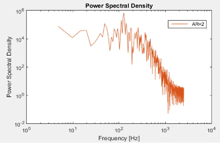
Figure 4.1 Power spectral density for AR = 2... 29

Figure 4.2 Time-averaged normalized streamwise velocity (U/U0) contours on central plane (y/d = 0) for (a) AR = 1, (b) AR = 2, (c) AR = 4; and on side-face plane (y/d = 0.5) for (d) AR = 1, (e) AR = 2, (f) AR = 4. ... 31

Figure 4.3 Time-averaged streamtraces for flow past a cylinder with AR = 7, (from Wang and Zhou [3]) ... 33

Figure 4.4 Time-averaged velocity vectors for flow past an immersed circular cylinder, (from Heidari [29]) ... 35

Figure 4.5 Time-averaged streamtraces of the recirculation in the flow field for (top row) AR = 1, (middle row) AR = 2, (bottom row) AR = 4 on their central planes (left column) and side-face planes (right column) ... 37

Figure 4.6 Time-averaged streamtraces for the recirculation in the flow field of AR = 4 in vertical planes (from y/d = 0 to 0.8) ... 38

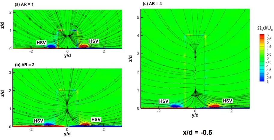
Figure 4.7 Streamtraces in the transverse plane at x/d = -0.5 ... 39

Figure 4.8 Streamtraces in the transverse plane at x/d = 0 ... 40

Figure 4.9 Streamtraces in the transverse plane at x/d = 0.3 ... 41

Figure 4.10 Streamtraces in the transverse plane at x/d = 0.6... 42

Figure 4.11 Streamtraces in the transverse plane at x/d = 1... 43

(13)

xii

Figure 4.13 Horizontal planes shaded by normalized normal velocity (W̅ /U₀) taken in the cases

of AR = 1 (top row), AR = 2 (middle row), and AR = 4 (bottom row) at the vertical location of

0.25h (left column), 0.5h (central column), and 0.75h (right column). ... 46

Figure 4.14 Pressure coefficient (Cp) distribution on (a) windward face of each cylinder;

(b) derivative of the pressure coefficient with respect to vertical location (ΔCp/Δ(z/h)) ... 48

Figure 4.15 Horizontal planes through Point A, coloured by normalized streamwise velocity

(𝑈̅/𝑈0): (a) AR = 1, (b) AR = 2, (c) AR = 4 ... 50

Figure 4.16 Horizontal planes through Point A, coloured by normalized streamwise velocity

(𝑈̅/𝑈𝑠): (a) AR = 1, (b) AR = 2, (c) AR = 4 ... 52

Figure 4.17 Horizontal planes through Point A coloured by normalized x-vorticity (Ωxd/U0): (a)

AR = 1, (b) AR = 2, (c) AR = 4 ... 55

Figure 4.18 Horizontal planes through Point B, coloured by time-averaged normalized

streamwise velocity (𝑈̅/𝑈0): (a) AR = 1, (b) AR = 2, (c) AR = 4 ... 56

Figure 4.19 Time-averaged normalized streamwise velocity (𝑈̅/𝑈0) plots crossing the wake

region of each cylinder from the downstream location of x/d = 0.6 to x/d = 2.2 ... 58

Figure 4.20 Horizontal planes through Point C (left column) and Point D (right column) for AR =

4 shaded by time-averaged normalized streamwise velocity (𝑈̅/𝑈0) (top row) and normalized

normal velocity (𝑊̅ /𝑈0)) (bottom row) ... 60

Figure 4.21 Time-averaged normalized spanwise vorticity (𝛺̅̅̅̅ × 𝑑/𝑈𝑦 0) contours in the central

plane: (a) AR = 1, (b) AR = 2, (c) AR = 4 ... 63

Figure 4.22 Normalized streamwise turbulence intensity ( √𝑢̅̅̅/𝑈2 ₀) contours in the central plane:

(a) AR = 1, (b) AR = 2, (c) AR = 4 ... 64

Figure 4.23 Normalized normal turbulence intensity (√w̅̅̅̅/U2 ₀) contours in the central plane: (a)

(14)

xiii

Figure 4.24 Normalized Reynolds shear stress−𝑢𝑤̅̅̅̅/𝑈02contours in the central plane: (a) AR = 1,

(b) AR = 2, (c) AR = 4. ... 67

Figure 4.25 Instantaneous flow field for AR = 1 coloured by spanwise vorticity (𝛺̅̅̅̅ × 𝑑/𝑈_𝑦 ₀): (a) shed vortex from the shear layer travels downstream; (b) shed vortex from the shear layer moves downward then travels downstream; (c) shed vortex from the shear layer curls and enters the near-wake ... 68

Figure 4.26 Instantaneous flow field for AR = 2 coloured by spanwise vorticity (𝛺̅̅̅̅ × 𝑑/𝑈𝑦 0): (a) shed vortex from the shear layer splits into two vortices, one travels downstream and one enters the near-wake; (b) shed vortex from the shear layer moves downward then travels downstream; (c) shed vortex from the shear layer curls and enters the near-wake ... 69

Figure 4.27 Instantaneous flow field for AR = 4 coloured by spanwise vorticity (𝛺̅̅̅̅ × 𝑑/𝑈𝑦 0): (a) shed vortex from the shear layer curls and enters the near wake; (b) shed vortex from the shear layer splits into two vortices,; (c) shed vortex from the shear layer splits into two vortices on the leeward face of the cylinder ... 71

Figure 4.28 Consecutive instantaneous flow fields for AR = 1 in the central plane with 0.001s between each field-of-view coloured by spanwise vorticity (𝛺̅̅̅̅ × 𝑑/𝑈_𝑦 ₀) ... 72

Figure 4.31 Time-averaged λ2 iso-surface of the flow field for AR = 4 ... 78

Figure 4.32 Time-averaged λ2 iso-surface of the flow field for AR = 2 ... 78

(15)

xiv

Nomenclature

AR Aspect ratio (-)

Cp Pressure coefficient (-)

d Cylinder width (m)

dwall Distance to the nearest wall (m)

E Energy (J)

f IDDES blending function (-)

h Cylinder height (m)

k Turbulence kinetic energy (m2/s2)

p Static pressure (Pa)

P0 Atmospheric pressure (Pa)

Pstag Pressure at the stagnation point (Pa)

𝑅𝛽, 𝑅𝜔 and 𝑅𝑘 Closure coefficients in viscous damping functions (-)

Red Reynolds number based on the cylinder width (-)

Reθ Reynolds number based on the boundary layer thickness (-)

ReT Turbulent Reynolds number (-)

ST Stress tensor (Pa)

St Strouhal number (-)

t Time (s)

𝑢_𝜏 Friction velocity (m/s)

𝑢, 𝑣, 𝑤 Fluctuating velocity components in x, y, z direction (m/s)

𝑈0 Freestream velocity (m/s)

𝑈_𝑠 Approach velocity at the corresponding location (m/s)

U_max Maximum velocity (m/s)

𝑈_𝑖 and 𝑈̅_𝑖 Instantaneous and time-averaged velocity in tensor notation (m/s)

U, V, W Instantaneous velocity components in x, y, z direction (m/s)

𝑈̅, 𝑉̅, 𝑊̅ Time-averaged velocity components in x, y, z direction (m/s)

√𝑢̅̅̅̅2

𝑈0 ,

√𝑣̅̅̅̅2

𝑈0 ,

√𝑤̅̅̅̅2

(16)

xv

𝑥𝑖 Position vector in tensor notation (m)

x, y, z Cartesian axis directions (m)

z+ Normalized wall normal distance (-)

λ2 Second eigenvalue of the pressure Hessian matrix (-)

ε Turbulence dissipation rate (m2/s2)

∅, ∅̅, ∅′ A scalar quantity, time-averaged and fluctuation of this quantity

𝜌 Fluid density (kg/m3)

𝜏 ̃ Reynolds stress tensor (Pa)

𝜇 Dynamic viscosity (m2/s)

𝜇𝑇 Eddy viscosity (m2/s)

𝜐 Kinematic viscosity (m2/s)

𝜔 Specific dissipation rate (1/s)

𝛺_𝑥, 𝛺_𝑦, 𝛺_𝑧 Vorticity in x, y, z direction (1/s)

(17)

1

Chapter 1 Introduction

A wall-mounted finite-length cylinder immersed in a flow produces a flow field

that is representative of that observed in many engineering applications in the real world,

such as wind flow past low-rise buildings, flow past electronic components and cooling

towers. The interaction between the fluid and the cylinder creates complex flow field

structures in the near wall region and in the turbulent wake behind the cylinder. The flow

structures greatly influence the performance of such a system with respect to, for example,

pedestrian comfort along a city street, heat transfer rate for electronic cooling, or

prediction of pollutant dissipation. It is also important to accurately predict the shedding

frequency of the vortices that develop behind the cylinder in order to avoid vibration

induced by resonance. Therefore, it is necessary to acquire an in-depth understanding of

wall-mounted bluff body flow in order to make improvements in practical application of

such flows.

The flow structure is mainly determined by three factors; Reynolds number (Red),

aspect ratio (AR = h/d, where h and d are the height and width of the cylinder,

respectively), and the relative boundary layer thickness (δ/d) [1]. At a low Reynolds

number, viscous forces dominate over inertial forces. In this case, the flow field tends to

be steady and very little turbulence is observed. As the Reynolds number increases,

inertial forces overcome the viscous forces and dominate the flow field. The flow field

becomes turbulent and more complex flow structures appear. El Hassan et al. [2]

experimentally studied the effect of relative boundary layer thickness on the flow field

around the square cylinder with AR = 4. They confirmed that the wake size is influenced

(18)

2

similar conclusion was found by Wang and Zhou [3]. It was concluded that as the

boundary layer thickness increases, the strength of the upwash flow behind the body is

enhanced, thereby weakening the effect of the downwash flow from the free-end of the

square cylinder.

The effect of aspect ratio of the cylinder on the flow field requires further

investigation. A critical value of AR, which is differentiated by the induced wake

structures, has been found to lie between the value of 3 and 5 [4]. Wang and Zhou [3]

showed that the flow past a cylinder with AR below the critical value is more likely to

create a symmetric arch-type wake, and that the flow past a cylinder with AR above such

value is more likely to create a wake similar to an asymmetric von Kármán vortex street.

An in-depth comparison of the flow field near the square cylinders below and

approaching the critical aspect ratio has not been established so far. In the current

research, the Reynolds number (Red) and boundary layer thickness (δ) of the incoming

flow will be fixed, and the square cylinders studied in this research have aspect ratios of 1,

2 and 4.

This research is conducted numerically with the commercial code Star-CCM+

v11.04 [5], running on the high-performance computing environment Shared Hierarchical

Academic Research Computing Network (SHARCNET). The first phase of this research

project is to validate the simulation model using the experimental results of El Hassan et

al. [2] at the cylinder aspect ratio of 4. After that, in the second phase, flow past a square

cylinder with AR = 1 and 2 are examined and compared to the square cylinder with AR =

(19)

3

The objectives of this research project are:

1. to model and validate the flow over a wall-mounted finite-length square

cylinder with the aspect ratio of four, using the Detached-Eddy Simulation

turbulence model;

2. to study the wake structure and the interaction between the vortical structures

around the square cylinder at different aspect ratios;

3. to provide an alternative method for horizontal plane selection which allows

researchers to better examine and compare the flow field around cylinders at

different aspect ratios.

This thesis consists of fourchapters. Chapter 1 provides a brief introduction to the

problem; Chapter 2 gives an overview of previous studies conducted on related problems

and discusses the turbulence model selection. Chapter 3 focuses on the numerical model

and grid setup, including the grid independence study and the validation of the model.

Chapter 4 discusses the simulation results. The time-averaged results on the vertical

planes and horizontal planes will be presented. Then, instantaneous turbulent quantities

are examined in order to gain a better understanding of the effect of aspect ratio on the

(20)

4

Chapter 2 Literature Review and Mathematical Model

2.1 Introduction

In this chapter, the relevant studies that have been conducted on this topic are

discussed. Previous experimental work has been used to obtain a general overview of the

physics of the flow field; the numerical work contributes to the model setup and provides

an understanding of the details in the flow field that was not obtained in the experiments.

The governing equations are also introduced in this chapter, along with a brief

introduction of the turbulence modeling applied to the current study.

2.2 Previous Experimental Studies

The flow over a square cylinder has been experimentally studied in terms of

evaluating characteristics of the vortical structures in the flow field. The flow structure is

mainly determined by three factors; Reynolds number based on the approach flow

velocity and cylinder width (Red), aspect ratio (AR = h/d, where h and d, are the height

and width of the cylinder, respectively), and the boundary layer thickness of the approach

flow (δ). The flow field structure around a wall-mounted cube was studied

experimentally by Castro and Robins [6]. To assess the effect of the approach flow, they

compared an incoming sheared turbulent flow with an irrotational uniform flow and

(21)

5

also found that the decay of velocity deficit behind the cube was strongly influenced by

turbulence intensity, as subsequently confirmed by Hunt et al. [7].

Lin et al. [1] performed an extensive study to determine how Red, δ and AR

influence the horseshoe vortex (HSV) system formed in front of the body for various

Reynolds numbers (200 < Red < 6,000) considering the flow over a wall-mounted

finite-height square cylinder. They identified four regimes in the HSV: a steady horseshoe,

periodic oscillation with small displacement, periodic breakaway vortex system and

irregular vortex system. This categorization was found to be strongly correlated with h/δ

and Red.

To determine the effect of the approach flow boundary layer thickness, Wang et al.

[8] studied the flow over a square cylinder with three different values of δ. They noted

the flow field to be highly three-dimensional and consisted of the vortical structures

which included the tip vortex (connected to the downwash flow), the spanwise vortex

(the von Kármán vortex street), the base vortex formed at the junction of the wall and the

cylinder base, an upwash flow and the horseshoe vortex. A cartoon illustrating the fluid

structures is shown in Figure 1. The upwash flow in the wake was found to be enhanced

with increasing boundary layer thickness, and the downwash flow near the free-end shear

layer was consequently weakened by the enhanced upwash flow. As the upwash flow

(22)

6

Figure 2.1 Schematic of the flow structure behind a wall-mounted finite square cylinder with AR > 5 [8]

Wang and Zhou [3] studied the flow past a square cylinder with various aspect

ratios for Red = 9300, δ/d = 1.35. From their experimental study, they concluded that the

size of the reverse flow zone behind the cylinder was largely dependent on the cylinder

AR when the aspect ratio was between 3 and 7. Within this range, both upwash and

downwash flow in the wake were increased with increasing AR. In their study, Wang and

Zhou [3] presented a more sophisticated model with two different configurations of the

arch-type vortex forming behind the square cylinder. An asymmetric configuration

dominated the wake when the cylinder AR exceeded a critical value (between 3 and 5),

while symmetric spanwise vortical structures were found to be dominant when the AR

(23)

7

Figure 2.2 Schematic of the flow structure around a wall-mounted finite square cylinder: (a) two symmetric spanwise vortices, (b) asymmetric spanwise vortices [3]

Bourgeois et al. [9] conducted an experimental investigation of air flow with a

thin boundary layer over a wall-mounted finite-height square cylinder. The flow field

near a square cylinder with AR = 4 was captured using a laser Doppler velocimeter

(LDV). This flow field served as a challenge problem at the CFD Society of Canada

Annual Conference in 2012, and the LDV results were used to benchmark the numerical

solutions submitted by participants. This study showed that the alternating vortex

shedding was deformed due to the free-end shear layer as it evolved downstream. The

flow field was decomposed by phase averaging, which captured the coherent and

incoherent structures in the flow field. Later, El Hassan et al. [2] continued this

investigation to study the effect of the boundary layer thickness on the wake structures.

(24)

8

thicker, similar to the observation of Wang and Zhou [3]. In the thinner boundary layer

case, the influence of the horseshoe vortex on the wake region was limited and as δ

increased, the entire wake structure was affected by the horseshoe vortex. Sumner et al.

[4] summarized the previous studies on flow past a wall-mounted finite circular cylinder

and stated that the studies on this topic are insufficient at the present time.

Sumner et al. [4] summarized the previous studies on flow past a wall-mounted

finite circular cylinder and stated that the studies on this topic are insufficient at present.

“Apart from the location of the reattachment point, the influences of Reynolds

number, aspect ratio, and relative boundary layer thickness are not well

understood… …most of the experiments in the literature have been concentrated on

cylinders of relatively low aspect ratio, AR ≤ 2, and there is a need for additional studies

at higher AR.”

- D. Sumner

2.3 Previous Numerical Studies

Shah and Ferziger [10] demonstrated the capability of utilizing the Large-Eddy

Simulation (LES) model in the flow past a wall-mounted cube with Reynolds number of

40,000. They showed that the mean and fluctuating quantities at different locations in the

flow field matched well with experimental results. Rodi [11] conducted a comparative

study on LES and Reynolds Averaged Navier-Stokes (RANS) turbulence models in the

case of flow past a wall-mounted square cylinder. All RANS models significantly

under-predicted the velocity fluctuations in the flow field. On the other hand, the LES model

(25)

9

though the unsteady RANS model could accurately predict the vortex shedding frequency.

However, although the LES calculations increased the computing time by a factor of

almost 40 compared with the RANS models, none of the LES results were entirely

satisfactory possibly due to the insufficient of resolution on the side-wall of the cylinder.

Fröhlich and Rodi [14] numerically studied the vortex shedding process using LES for

flow past a finite-height wall-mounted circular cylinder with an aspect ratio of 2.5. Their

study revealed the interaction of the separating shear layer from the side wall with that

from the free-end. The two-dimensional alternating vortex shedding was distorted as they

travelled downstream. The simulation predicted an arch-type vortex behind the cylinder.

Nishino et al. [12] conducted numerical simulation using unsteady RANS and

DES for flow past a circular cylinder placed near and parallel to the bed with various

gaps. The unsteady RANS model was not capable of predicting the ground effect while

the DES result showed a good match with experimental results, by examining the

cessation of large-scale alternating vortex shedding behind the cylinder. The authors also

noted that the vortical structures resolved in the unsteady RANS were much coarser than

those by the DES, although the same grid was employed and the same computational cost

was required for each. A significant improvement in the simulation with DES model was

displayed over that with unsteady RANS model. Nasif et al. [13]modeled the flow past a

sharp edge bluff body in a shallow open channel with DES. The flow field was visualized

by creating an iso-surface of the λ2 – criterion. Various vortical structures in the

near-wake and far-near-wake were identified by the authors.

An in-depth comparison of the flow field near the square cylinders below and

(26)

10

research, the Reynolds number (Red) and boundary layer thickness (δ) of the incoming

flow are fixed, while the aspect ratio was varied from 1 to 4. The principal objective of

this research project was to study the wake structure and the interaction between the

vortical structures around the square cylinder at different aspect ratios. The study also

focussed on developing an alternative method for horizontal plane selection to visualise

the flow field which would allow researchers to better examine and compare the flow

field around cylinders at different ARs.

2.4 Governing Equations and Turbulence Modeling Techniques

The mathematical model of fluid flow and heat transfer is developed from the

conservation of mass, Newton’s second law and the first law of thermodynamics. After

adequate treatment to these general physics laws, they become the continuity equation,

momentum equation, and conservation of energy equation. In the conservative form, they

are expressed by:

Continuity equation:

𝜕𝜌

𝜕𝑡+ 𝑑𝑖𝑣(𝜌𝑈𝑖) = 0 (2.1)

Momentum (Navier-Stokes) equations:

𝜕

𝜕𝑡(𝜌𝑈𝑖 ) + 𝑑𝑖𝑣(𝜌𝑈𝑖𝑈𝑖) = − 𝜕𝑝

𝜕𝑥+ 𝑑𝑖𝑣(𝜏 ̃) + 𝜌𝑔𝑖 (2.2)

Conservation of energy:

∂

(27)

11

The definition of the parameters in these equations is given in the Nomenclature.

Although heat transfer of flow passing a square cylinder can be studied, the current study

only focuses on the flow field structure and physics of the flow field. Therefore the

energy equation will not be discussed further.

The solution of the governing flow equations can be decomposed into

time-averaged and fluctuating components:

𝑢⃑ = 𝑈̅ + 𝑢 (2.4)

∅ = ∅̅ + ∅ (2.5)

where ∅ represents any scalar quantity, the overbar notation represents the mean value,

and the prime symbol represents the fluctuating component.

Using Equations 2.4 and 2.5, the time-averaged continuity equation and

momentum equation for incompressible flow are expressed as:

∂𝑈̅𝑖

𝜕𝑥𝑖= 0 (2.6)

𝜌𝑢̅𝑗∂𝑈̅_𝜕𝑥𝑖 𝑗= − ∂𝑝̅ 𝜕𝑥𝑖+ 𝜇 𝜕 𝜕𝑥𝑗( 𝜕𝑈̅𝑖 𝜕𝑥𝑗+ 𝜕𝑈̅𝑗 𝜕𝑥𝑖) + [−𝜌 𝜕

𝜕𝑥𝑗(𝑢̅̅̅̅̅)] + 𝜌𝑔 𝑖𝑢𝑗 𝑖 (2.7)

The second last term [−𝜌_𝜕𝑥𝜕

𝑗(𝑢̅̅̅̅̅)]𝑖𝑢𝑗 in the time-averaged momentum equation

(2.7) contains the fluctuating components, known as the Reynolds stresses. This term

must be computed in turbulent flow and is the main source of difficulties in modeling

such flows [15].

The most common approaches to simulate turbulent flow are Reynolds Averaged

(28)

hybrid-LES-12

RANS, known as the Detached Eddy Simulation (DES) model [16]. The definition of a

complete turbulence model is one which “can be used to predict properties of a given

turbulent flow with no prior knowledge of the turbulence structure” [17]. Although

RANS models have several options including the 0-, 1/2- and 1-equation models, only

the k-ϵ and k-ω two-equation models are considered as complete RANS models. In

addition to the transport equation for turbulence kinetic energy (k), the k-ω models

consist of a second transport equation for specific dissipation rate (ω), while k-ϵ models

consist of a transport equation for dissipation rate (ϵ). Over decades of benchmarking

these two models, the standard k-ϵ model is known to be sensitive in the near-wall region

and the standard k-ω model is sensitive to the inlet freestream turbulence properties.

Mentor [18] developed the idea of combining these two turbulence models in order to

include the advantages of each, and showed that k-ω shear stress transport (SST)

performs better than k-ϵ when an adverse pressure gradient occurs.

Since all the RANS models utilize the Boussinesq eddy viscosity assumption to

model velocity fluctuations, the value of turbulence kinetic energy is assumed to be the

same in all three directions (x, y, and z). Although this is a convenient way of modeling

turbulence and providing a robust prediction, the commonly known drawbacks of RANS

(including unsteady RANS) models are:

1. Lack of potential for further analysis of the turbulence quantities

2. Lack of accuracy when adverse pressure gradients exist (although better than k-ϵ,

k-ω SST over-predicts turbulence quantities)

The Large Eddy Simulation (LES) model explicitly resolves the large eddies in a

(29)

13

behind an LES model can be understood as follows: the large eddies in the flow field are

geometry dependent, so the Navier-Stokes equations can be solved directly, and the

smaller eddies can be modeled (with Boussinesq eddy viscosity assumption) since they

are treated as isotropic. Shah and Ferziger [10] showed that with appropriate grid

utilization, an LES model is capable of accurately simulating the flow past a

wall-mounted cube. With the LES model, details of turbulence quantities can be acquired as

opposed to RANS models in which only time-averaged information is available.

However, an LES model requires large computational resources. In order to successfully

predict the flow field with an LES model, the computational grid must be carefully

designed because of the filtering process. With an inadequate grid setup in the near-wall

region, the result of an LES simulation can potentially be much less accurate than any

RANS simulation. RANS models are commonly understood as naturally independent of

grid spacing, while LES requires the grid spacing to meet a specific standard in order to

produce meaningful results [19].

Detached Eddy Simulation (DES) is a hybrid scheme which implements a RANS

model in the near-wall region (which allows more flexibility on the grid spacing), and

employs an LES model to resolve the large unsteady eddies away from the wall. Only the

RANS models which appropriately define the turbulence length scale can be considered

in the DES model, such as Spalart-Allmaras (S-A) and k-ω SST. Spalart et al. [20]

introduced an Improved Delayed Detached Eddy Simulation (IDDES), which improves

the computation at the cells where the transition between the RANS and LES models

occurs. A blending function 𝑓 is used to switch between the selected unsteady RANS and

(30)

14

𝑓 = min[2𝑒𝑥𝑝(−9𝛼𝐼𝐷𝐷𝐸𝑆2) , 1.0] (2.8)

𝛼𝐼𝐷𝐷𝐸𝑆= 0.25 −𝑑𝑤𝑎𝑙𝑙_∆ (2.9)

where 𝑑𝑤𝑎𝑙𝑙 represents the shortest distance from the specified cell to the nearest wall,

and ∆ represents the grid spacing. The value of the blending function lies between 0 and

1, where 0 indicates that the corresponding cell is LES-dominant and 1 represents

unsteady RANS-dominant.

In this research project, IDDES with k-ω SST model will be used to simulate the

turbulent flow around a wall-mounted square cylinder. IDDES is chosen over the RANS

models because:

1. The details of turbulence quantities such as velocity fluctuations are important for

analyzing the flow field structures;

2. Strong separations are expected, which is a known weakness of any RANS model.

As expected, a well-setup LES model is known to have better performance than

an IDDES model. Saeedi and Wang [21] conducted an LES study of flow past a

wall-mounted finite square cylinder with AR = 4. A small computational domain was used in

their study and the domain was meshed with 14.3 million computational cells. This

reflects that very small grid spacing was applied in the domain to satisfy the mesh

restrictions imposed by LES. Consequently, in order to keep a relatively safe

Courant-Friedrichs-Lewy number (generally smaller than 1), the time step size had to be reduced,

which means a very long period of time is required to complete the simulation. Their LES

(31)

15

adequate accuracy has been obtained with the IDDES model, while maintaining a higher

computational efficiency than the LES model.

Chapter 3 Numerical Setup

3.1 Introduction

The computational domain for any simulation should be chosen with care. The

boundaries of the domain should be placed adequately far from the cylinder in order to

eliminate the influence from the boundaries, but not so far away as to incur the

unnecessary additional computational expense. Although COST [22] provides good

standards for this setup, the process of selecting an appropriate computational domain

requires experience and testing. This chapter presents the computational domain and

boundary conditions used in this investigation, along with the meshing methods and the

grid independence study. At the end of this chapter, the computational model is validated

against the experimental results of Bourgeois et al. [9] and El Hassan et al. [2].

3.2 Computation Domain

Based on the experimental work of El Hassan et al. [2] and Bourgeois et al. [9], a

wall-mounted finite square cylinder with a width of d = 0.0127 m is selected for this

study. The air flow has Reynolds number of 12,000 based on the freestream velocity (𝑈₀)

of 15 m/s and the cylinder width, with freestream turbulence intensity of 0.8% and

dynamic viscosity of 1.855 x 10-5Pa-s. The current study focuses on square cylinders with

AR = 1, 2 and 4 immersed in the flow field with the above properties.

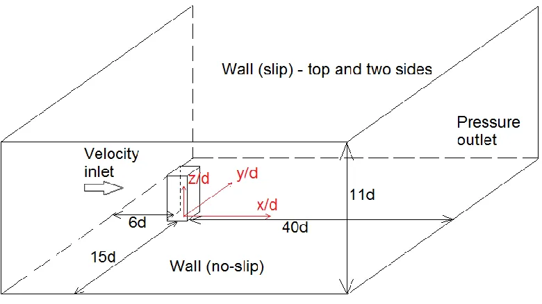
Figure 3.1 shows a schematic of the computation domain. In this study, the origin

(32)

16

x-, y- and z-coordinate directions correspond to the streamwise, spanwise and vertical

directions, respectively. The inlet boundary is placed 6d upstream before the cylinder’s

windward surface (i.e. at x = -6.5d). Upstream distances of 10d and 20d have also been

tested, where no significant influence on the flow field was found. The two slip walls on

the side are placed 15d away (i.e. at y = ±15.5d) from each side-face of the cylinder,

maintaining a blockage ratio of 3%. The outlet boundary is placed 40d downstream (i.e.

at x/d = 40.5) of the cylinder’s leeward surface to ensure elimination of reverse pressure

gradients on the outlet boundary. The height of the domain is 11d, in order to ensure there

is an adequate distance from the free-end shear layer of the AR = 4 cylinder, so that the

streamwise velocity measured at the top wall is the same as the freestream velocity in the

experiment.

Figure 3.1 Schematic of the computation domain

3.3 Boundary Conditions

The side and top walls of the computational domain are smooth slip walls

(33)

17

walls (Dirichlet boundary condition). The outlet boundary is specified as a pressure outlet

(Neumann boundary condition), and the static pressure in each outlet cell is set at 0 Pa.

The inlet condition has to be carefully assigned to match the flow field in El

Hassan et al.’s experiment [2]. Figure 3.2 shows the boundary layer profile of the

streamwise velocity (U+= 𝑈̅/uτ) and the turbulence intensity (√𝑢̅̅̅/𝑈2 0) versus 𝑍+ =𝑧∗𝑢_𝜐𝜏

at the cylinder’s location for the flow along a flat plate without the cylinder, where uτ and

𝜐 represent friction velocity and kinematic viscosity, respectively. According to El

Hassan et al. [2] and Bourgeois et al. [9], the boundary layer thickness (δ = 9.11 mm) at

this location is 72% of the cylinder width.

Figure 3.2 Experimental results [2] compared to wall function, DNS predictions [23] and other experimental results [24]; (a) time-averaged streamwise velocity, and (b)

turbulence intensity

The two experimental profiles above demonstrate good agreement with the result

of an Improved Delayed Detached Eddy Simulation (IDDES) study of flow along a flat

plate [23] as well as the log law of the wall. However, simulations using the currently

available standard RANS models show that the turbulence intensity profiles are poorly

matched at this 𝑅𝑒𝜃 value (𝑅𝑒𝜃 = 𝛿 ∗ 𝑈0/𝜐 ≈ 1000), as seen in Fig. 3.3. The peak

(34)

18

Figure 3.3 Comparison between k-ω SST predictions, at the cylinder location with the cylinder removed, and the experimental results by El Hassan et al. [2]; (a) time-averaged

streamwise velocity, and (b) turbulence intensity

In a standard k-ω model, the turbulence kinetic energy (k) is quickly diffused in

the near-wall region by an excessively large value of specific turbulence dissipation rate

(ω) [17]. This formulation is valid when 𝑅𝑒𝜃 (based on the boundary layer thickness) is

significantly greater than 10,000. When 𝑅𝑒_𝜃 is relatively small, the turbulence dissipation

rate ω tends to damp out an extra amount of turbulence kinetic energy and leads to the

under-prediction of turbulence intensity by the Boussinesq approximation, as seen from

the expression

𝑇. 𝐼. = √𝑢̅̅̅/𝑈2

0= √2₃𝑘 (3.1)

To overcome the deficiency of the model for low 𝑅𝑒_𝜃, Wilcox [17] modified the

k-ω model with three extra variables: 𝑅𝛽, 𝑅𝜔, and 𝑅𝑘. These variables are designed to

help restrict the value of specific dissipation rate at the wall while not disturbing the main

flow field. The governing equations for k and ω are modified to:

𝑈̅𝜕𝑘_𝜕𝑥+ 𝑉̅𝜕𝑘_𝜕𝑦= 𝑣𝑇(𝜕𝑈̅_𝜕𝑥)2− 𝛽∗𝜔𝑘 +_𝜕𝑦𝜕 [(𝑣 + 𝜎∗𝑣𝑇)𝜕𝑘_𝜕𝑦] (3.3)

(35)

19

where 𝛼∗, 𝛼, 𝛽∗ are defined as:

𝛼∗ ₌𝛼0∗+𝑅𝑒𝑇/𝑅𝑘

1+𝑅𝑒𝑇/𝑅𝑘 (3.5)

𝛼 =5₉𝛼0+ 𝑅𝑒𝑇

𝑅𝜔

1+𝑅𝑒𝑇_𝑅𝜔 (𝛼

∗₎−1_(3.6)

𝛽∗₌ 9 100

5

18+(𝑅𝑒𝑇_𝑅𝛽)4

1+(𝑅𝑒𝑇

𝑅𝛽)4

(3.7)

where the values of the constants are:

𝛽 = 3

40, 𝜎 = 𝜎∗ = 1 2, 𝛼0∗ =

1

40, 𝛼0 = 1 10

The turbulent Reynolds number ReT in these equations is defined as:

𝑅𝑒𝑇 =_𝜔𝜐𝑘 (3.8)

From testing, the optimized values of 𝑅_𝛽, 𝑅_𝜔 and 𝑅_𝑘 are:

𝑅_𝛽 30

𝑅𝑘 12

𝑅_𝜔 2.95

With the optimized values of 𝑅𝛽, 𝑅𝜔 and 𝑅𝑘, the k-ω model with low-Reynolds

number modification is capable of predicting the streamwise velocity and turbulence

intensity with sufficient accuracy as shown in Fig. 3.4, although the peak value of

turbulence intensity is still under-predicted by about 15%. By raising the value of 𝑅_𝛽 to

(36)

20

velocity profile will be heavily affected. Although it is possible to determine the best set

of values by trial and error, a compromise has to be made because the major influence to

the flow is the bluff body, not the turbulence intensity profile of the boundary layer.

Figure 3.4 Streamwise velocity (left) and turbulence intensity (right) profiles plotted at the cylinder’s location, with the cylinder removed.

The streamwise velocity (𝑈), turbulence kinetic energy (𝑘) and specific

turbulence dissipation rate (𝜔) profiles are taken at the location 6.5d upstream of the

cylinder and mapped onto the inlet boundary of the computational domain. This ensures

that the flow has the same characteristics as the experiment at the cylinder’s location.

3.4 Grid

A polyhedral, unstructured, surface-controlled mesh is used for this study. Our tests

have shown that the polyhedral unstructured mesh allows better clustering at the cylinder

corners and proper transition from the prism layers near the surfaces. The

surface-controlled mesh yields results that are closer to the experiment than the results from a

volume-controlled mesh. The grid spacing is defined on the cylinder surface and the bed.

Ten prism layers are placed on the no-slip walls with adequate spacing to ensure more

(37)

21

computational domain have a slow growth rate outward from the wall. Figure 3.5 shows

the centre plane of the AR= 4 cylinder with the surface cell size of 1 mm.

Figure 3.5 Illustration of the polyhedral grid on the central plane

A study of grid independence provides information on the optimal cell size

relative to computational accuracy. Since DES uses an implicit time-marching scheme,

the Courant-Freidrichs-Lewy (CFL) number may exceed 1 as long as the residuals of the

governing equations converge to zero. Table 3.1 presents the parameters used for each

mesh tested in this study. Meshes 1, 2 and 3-a represent coarse, finer and finest mesh

respectively, with the same time step size of 2 x 10-4 s. Mesh 3-b was also used with the

time step size at 1 x 10-4 s to understand the effect of CFL number on the result.

(38)

22

Figs. 3.6(a) and (b) show profiles on the middle plane behind the AR = 4 cylinder

at different elevations. The profiles of Mesh 1 at all levels are significantly off from other

schemes. Mesh 2 is slightly different from Mesh 3-a, Mesh 3-b, and the experimental

result between x/d = 0.5 and x/d = 4, which encompasses the wake region. Reducing the

grid spacing from 1 mm to 0.5 mm on the cylinder’s faces provides a subtle improvement.

However, the effect of time step size is almost negligible because the velocity profiles of

Mesh 3-a and Mesh 3-b are very close to each other.

Figure 3.6 Comparison of the time-averaged streamwise velocity (𝑈̅/𝑈0) and turbulence intensity (√𝑢̅2/𝑈₀) with different meshes and experimental result

In the horizontal planes, almost all mesh schemes predicted the mean velocity in

(39)

23

quantities: in Figs. 3.6 (c) and (d), √𝑢̅̅̅/𝑈2 0 was slightly over-predicted by Mesh 2, 3-a

and 3-b. It is difficult to distinguish which one amongst Mesh 2, 3-a, and 3-b is

significantly better, but all closely represents the result from Bourgeois et al.’s

experiment [9].

In conclusion, Mesh 1 is too coarse to produce a reliable and accurate result. The

results from Meshes 2, 3-a and 3-b are closer to the experimental values measured by

Bourgeois et al. [9]. Since Mesh 2 is more computationally efficient than Mesh a and

3-b due to the reduction in cell count, cylinders with AR = 2 and 4 use Mesh 2. To increase

the number of cells on the side wall of the cylinder which is smaller in size, the cylinder

with AR = 1 uses Mesh 3-a. Mesh 3-b does not show any superiority over other mesh

schemes, and it almost doubles the computational time over that of Mesh 3-a.

3.5 Validation

The experimental study of Bourgeois et al. [9] served as a benchmark in a

challenge problem at the CFD Society of Canada Annual Conference in 2012.

Subsequently, Bourgeois et al. [24] and El Hassan et al. [2] compiled the results and

conducted further studies on the flow field around the cylinder with AR = 4. The same

problem was also studied by Saeedi and Wang [21] with LES and by Saeedi et al. [26]

using DNS. The experimental results from the study by Bourgeois et al. [9] and the LES

results by Saeedi and Wang [21] were used to validate the current DES results.

Fig. 3.7 shows the streamtraces on the centre plane y/d = 0 shaded by the

streamwise velocity contour, with the DES simulation result on the left and the

(40)

24

point in both figures is located at the same level (z/d ≈ 2). Flow above the stagnation

point moves upward and reaches the leading edge of the free-end. Behind the cylinder,

the flow moves sharply downward around x/d = 3 and recirculates to the leeward side of

the cylinder at z/d = 1. An upwash flow structure beneath the recirculation bubble is

observed at x/d ≈ 3 in both figures.

Figure 3.7 Validation of the current DES result (left) against the experimental result (right) by Bourgeois et al. [9] at the centre plane y/d = 0

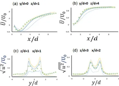
The time-averaged normalized streamwise velocity 𝑈̅/𝑈0 was tracked behind the

body on the middle plane at the levels of z/d = 2 and z/d = 3 as shown in Fig. 3.8. The

DES results show good agreement with Bourgeois et al.’s experimental results [9]. At

both levels, 𝑈̅/𝑈₀ has zero value on the wall and then becomes negative due to the

reverse flow from the recirculation. After x/d ≈ 3, 𝑈̅/𝑈₀ becomes positive again and

(41)

25

Figure 3.8 Time-averaged normalized streamwise velocity (𝑈̅/𝑈₀) on y/d = 0 plane, behind the cylinder at the vertical level of (a) z/d = 2 and (b) z/d = 3.

On the horizontal plane z/d = 3, time-averaged normalized streamwise and

spanwise velocity (𝑈̅/𝑈₀ and 𝑉̅/𝑈₀) and root-mean-square of the fluctuation of the

streamwise and spanwise velocity (√𝑢̅̅̅/𝑈2 ₀ and √𝑣̅̅̅/𝑈2 ₀) are tracked at the location of

x/d = 2. Fig. 3.9 compares the results from the current DES study with the experimental

(42)

26

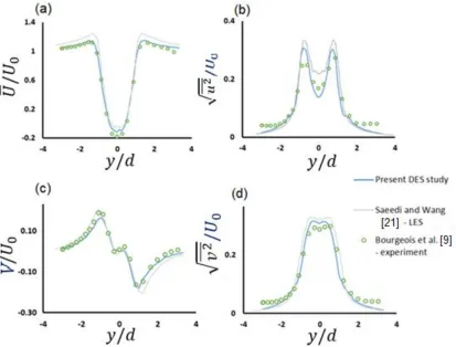
Figure 3.9 Validation of the current DES model with experimental result and an LES study on the plane z/d = 3 at the location x/d = 2: (a) time-averaged streamwise velocity

(𝑈̅/𝑈₀) and (b) fluctuating streamwise velocity root-mean-square(√𝑢̅̅̅/𝑈2 ₀); (c) time-averaged spanwise velocity (𝑉̅/𝑈₀); (d) fluctuating spanwise velocity root-mean-square

(√𝑣̅̅̅/𝑈2 ₀)

The current DES study shows good agreement with the experimental streamwise

and spanwise velocity profiles. At the two ends of the profiles, the values of normalized

streamwise velocity become very close to unity. The lowest streamwise velocity inside

the wake region is located at y/d = 0. At the location of x/d = 2, both DES and LES

slightly under-predict the peak streamwise velocity. This feature is also shown on the

central plane (Fig. 3.7) as a slightly extended recirculation zone in Bourgeois et al.’s [9]

experiment velocity contour. The fluctuation of streamwise and spanwise velocities

(43)

27

Overall, the mismatch is considerably low compared with the LES solution. Thus, the

current DES model has been validated and is regarded as capable of predicting the size

(44)

28

Chapter 4 Results and Discussion

4.1 General Remarks

In this chapter, the time-averaged and the instantaneous flow field characteristics

are discussed. As the fluid negotiates around the wall-mounted cylinder, it experiences

separation from three edges, the formation of the horseshoe vortex near the bed in front

of the body and formation of a wake region behind the cylinder. However, the effect of

the flow separating from the top edge of the cylinder and the effect of the bed on the

wake characteristics can vary depending on the aspect ratio. The characteristics of

interest include the dominant shedding frequency of the wake vortices, the pressure

distribution on the body, and the mean and instantaneous velocity field in the wake. The

flow field is also visualized using the 2 criterion to develop an overall picture of the

wake structure. These aspects are discussed in this chapter.

4.2 Vortex Shedding Frequency

In the simulation, probes were placed in the wake region behind the cylinder for

the purpose of tracking the spanwise velocity. Using this velocity time history, the power

spectral density was calculated, and a sample is illustrated in Fig. 4.1. The dominant peak

corresponding to the vortex shedding frequency (~120 Hz) was found to be the same for

all three values of AR. The corresponding Strouhal number (St = fd/𝑈₀) is calculated to

be 0.103, which matches well with the 0.104 obtained by El Hassan et al. [2] for AR = 4.

This serves as an additional validation of the simulation results. The value of St is lower

than that measured in the flow past an infinitely long square cylinder, which is in the

range 0.125 to 0.130 [27]. However, Zdravkovich [28] observed that the downwash flow

(45)

29

formation and widens the wake, which consequently reduces the frequency of vortex

shedding. A similar effect has been recorded by other experimental researchers, e.g. [4].

The fact that the Strouhal number does not change with cylinder height is an indication

that the aspect ratio has little effect on the vortex shedding characteristics.

Figure 4.1 Power spectral density for AR = 2

4.3 Time-averaged Velocity Field

To ensure that the flow field has statistically achieved a steady state, the time

averaging of the velocity data was commenced after 100 cycles of vortex shedding. The

time-averaged results from over 60 vortex shedding cycles was calculated and is

presented in the following sections.

4.3.1 Velocity Field in Central Planes and Side Faces

The time-averaged streamwise velocity contours, with superimposed streamtraces,

on the central plane (y/d = 0) and the side-face plane (y/d = 0.5) of each cylinder are

(46)

30

aspect ratios: the presence of the horseshoe vortex (HSV), the formation of the separating

streamline at the top edge followed by the downward flow into the wake region and the

formation of the recirculation region immediately behind the body.

As the incoming flow impinges on the windward face of each cylinder, the flow

splits and a portion of the fluid moves upwards and over the free-end. There is also a

significant amount of the approach flow which moves downwards and rolls up into a

horseshoe vortex close to the bed. The horseshoe vortex can also be seen on the side-face

plane, but the vortex is somewhat reduced in size in Figs. 4.2(d), (e) and (f) as the

horseshoe vortex tube turns from the spanwise direction towards the streamwise direction

(47)

31

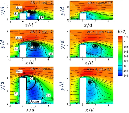
Figure 4.2 Time-averaged normalized streamwise velocity (𝑈̅/𝑈₀) contours on central plane (y/d = 0) for (a) AR = 1, (b) AR = 2, (c) AR = 4; and on side-face plane (y/d = 0.5)

for (d) AR = 1, (e) AR = 2, (f) AR = 4.

At the cylinder’s free-end, due to flow separation, a shear layer is formed. The

magnitude of the local peak velocity (Umax/𝑈0) in this region increases as the cylinder AR

increases, albeit slightly, due to the increasing pressure difference between the windward

and leeward faces. The location of the peak velocity moves further away from the

free-end of each cylinder in the downstream and normal directions as the cylinder AR

(48)

32

Table 4.1 Magnitudes and coordinates of Umax

AR Umax/U0 x/d (z - h)/d

1 1.18 0.013 0.41

2 1.20 0.060 0.55

4 1.27 0.113 0.57

As noticed in Fig. 4.2, the downwash flow creates a recirculation in the wake

region close to the top edge of the body. The core of the recirculation is marked by “C” in

Figs. 4.2 (a), (b) and (c). The size and location of the recirculation induced by the

downwash flow vary with AR. Table 4.2 lists the coordinates of the vortex core in each

case, where the values of the streamwise and normal velocity are found to be zero, and

the local pressure is found to be a minimum.

Table 4.2 Coordinates of the vortex cores (marked as C in Figs. 4.2 (a), (b) and (c)).The experimental result [3] for AR = 7 is indicated with an asterisk)

AR x/d z/d z/h

1 1.26 1.16 1.16

2 1.73 1.93 0.97

4 0.99 3.49 0.87

7* 1.07* 6.79* 0.97*

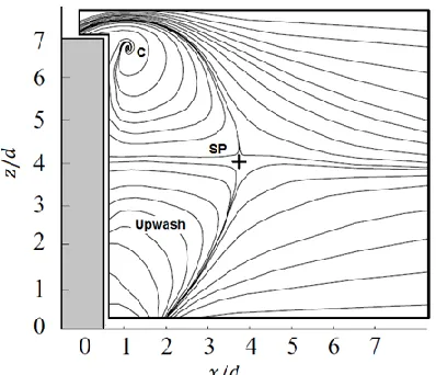
A saddle point (indicated by SP) occurs in the flow as shown in Fig. 4.3

(extracted from [3]) for AR = 7. This figure confirms the pattern of both the recirculation

zone and the variation of the location of the saddle point with AR noticed in the present

study. The streamwise location of a saddle point in the wake indicates whether the flow

tends to move towards the body or outwards in the streamwise direction, while the

vertical location of the saddle point indicates the location where the downward-moving

flow and the upward-moving flow meet. In Figs. 4.2(a, b), the saddle point is not clearly

identifiable and is located on the bed for cylinders with AR = 1 and 2, which shows that

(49)

33

Figure 4.3 Time-averaged streamtraces for flow past a cylinder with AR = 7, (from Wang and Zhou [3])

Table 4.3 Coordinates of the saddle points

AR x/d z/d (h-z)/d

1 2.20 0.00 1.00

2 3.40 0.00 2.00

4 3.22 0.91 3.09

7* 3.70* 4.03* 2.97*

As the cylinder AR is increased from 1 to 2, the value of Umax increases as shown

in Table 4.1. This causes the separating streamline to travel farther away from the body.

The streamline eventually turns and impinges on the bed forming the recirculation region,

which causes the vortex core and the saddle point to move farther downstream from x/d =

1.26 to x/d = 1.73, and from x/d = 2.2 to x/d = 3.4, respectively. However, when AR = 4,

as indicated by the location of the Umax in Table 4.1, the streamline initially travels

upwards and then quickly turns towards the bed. This causes the vortex core to move

closer to the body (x/d = 1) and the recirculation region to become slightly smaller than

that noticed in the AR = 2 case. Correspondingly, the streamwise location of the saddle

point moves slightly towards the cylinder at x/d ≈ 3. As the cylinder AR is further

increased to 7 [3], the streamwise location of the saddle point remains roughly at the

(50)

34

the top edge of the cylinder remains the same as well. This further indicates that the size

of the recirculation region is not significantly influenced by the cylinder AR when AR is

increased above a value of 4.

The downwash flow due to the presence of the cylinder free-end restrains the

upward motion of the flow from the bed. As the cylinder AR increases to 4 in Fig 4.2 (c),

the downwash flow is not strong enough to dominate the entire wake due to the

increasing distance between the free-end and the bed. Therefore, a flow structure with an

upward movement, commonly designated by researchers as upwash (Sumner [4],

Bourgeois et al. [9]), appears in the near-bed wake region. The upwash flow structure can

also be observed Fig.4.3 from the study of Wang and Zhou [3] at AR = 7. The upwash

structure presented by Wang and Zhou [3] has its origin close to the leeward face of the

cylinder at approximately x/d = 2, as opposed to at x/d = 3.5 for AR = 4 in the present

study. The shape of the upwash structure at AR = 7 is similar to the upwash structure in

the flow field of an emergent body with AR = 11 as shown in Fig. 4.4 [29]. By

comparing the upwash structure of AR = 4 with the upwash of taller bodies, it is obvious

that the upwash flow for AR = 4 is not fully evolved due to the influence of the

(51)

35

Figure 4.4 Time-averaged velocity vectors for flow past an immersed circular cylinder, (from Heidari [29])

Fig. 4.5 presents the streamtraces of the recirculation near the free-end of the

body for AR = 1 (a and d), AR = 2 (b and e), and AR = 4 (c and f) on central planes (a, b

and c) and side-face planes (d, e and f). By closely examining the recirculation in the

central plane and the side-face plane for each case, a change in flow pattern can be found

when the cylinder AR is increased from 2 to 4. As noted by Perry and Fairlie [30], an

inward-spiral vortex commonly termed as a stable focus is seen in Fig. 4.5(c). An

outward-spiral vortex, termed as an unstable focus, is noticed in Fig. 4.5(d). In the central

plane of the cylinder with AR = 1 and 2, both recirculation vortices are identified as

unstable foci. They are consistent with the recirculation found in their respective

side-face planes. However, the recirculation of the cylinder with AR = 4 is presented as a

stable vortex in the central plane but as unstable in the side-face plane. Fig. 4.6 presents

sections of the recirculation in the case of AR = 4 from the central plane (y/d = 0) to the

plane that is 0.3d beyond the side-face plane. The cross-section of the recirculation from

(52)

inward-36

spiraling. As the field-of-view is translated from y/d = 0 to y/d = 0.3, the streamtraces are

found to be denser, which means an arbitrary fluid particle along the streamtrace takes a

longer route to enter the vortex core from the outer region. From y/d = 0.4 to y/d = 0.6

shown in Figs. 4.6(e) to (g), the cross-sections of the recirculation is outward-spiraling.

Also, the streamtraces become less dense as the field-of-view moves away from the

central plane, which is different from the observations on the planes from y/d = 0 to y/d =

0.3. For y/d > 0.6, the recirculation can no longer be captured as in Figs. 4.7(h) and (i).

The inward-spiraling vortex is considered stable since it experiences an axial expansion

strain, which amplifies its vorticity. The outward-spiraling vortex experiences an axial

(53)

37

Figure 4.5 Time-averaged streamtraces of the recirculation in the flow field for (top row) AR = 1, (middle row) AR = 2, (bottom row) AR = 4 on their central planes (left column)

(54)

38

Figure 4.6 Time-averaged streamtraces for the recirculation in the flow field of AR = 4 in vertical planes (from y/d = 0 to 0.8)

Figs.4.7-4.11 show the streamtrace pattern in the transverse (y-z) planes for each

AR from the location of the windward face of each cylinder (x/d = -0.5) to a downstream

location (x/d = 1). The transverse planes at other locations were examined, but the ones

that are presented in this section are the ones in which the streamtrace pattern shows

(55)

39

Figure 4.7 Streamtraces in the transverse plane at x/d = -0.5

Fig.4.7 shows the streamtrace pattern on the windward face of the body. The

pattern for each AR on the transverse plane shows many similarities. At AR = 1, there is

the presence of a horizontal line source around z/d = 0.7, while at the higher AR values

there is a tendency to form a vertical line source. At the near-bed level, there is a

significant curl in the streamtrace on each side of the cylinder at all three values of AR

and represents the horseshoe vortex. As will be seen in the upcoming figures, this pair of

(56)

40

Figure 4.8 Streamtraces in the transverse plane at x/d = 0

In Fig.4.8, in the transverse plane through x/d = 0, three pairs of vortices are

visible at AR = 1. There is one vortex pair on the top of the cylinder and two on the sides.

At the cylinder’s free-end, the pair of counter-rotating vortices are formed due to the

corner effect. This pair of vortices can be observed clearly in the transverse plane at x/d =

Effect of Aspect Ratio on the Flow Structures Behind a Square Cylinder

Scholarship at UWindsor

Scholarship at UWindsor

Effect of Aspect Ratio on the Flow Structures Behind a Square

Effect of Aspect Ratio on the Flow Structures Behind a Square

Cylinder

Cylinder

Author’s Declaration of Originality

Abstract

Dedication

Acknowledgements

Table of Contents

List of Figures

Nomenclature

Chapter 1

Introduction

Chapter 2

Literature Review and Mathematical Model

Chapter 3

Numerical Setup

Chapter 4

Results and Discussion