Article
IWSNs with On-sensor Data Processing for Machine
Fault Diagnosis
Liqun Hou1, Junteng Hao1, Yongguang Ma1 and Neil Bergmann2,*
1 School of Control and Computer Engineering, North China Electric Power University, Baoding, 071003,
China; [email protected]
2 School of Information Technology and Electrical Engineering, The University of Queensland, Brisbane,
4072, Australia; [email protected]
* Correspondence: [email protected]; Tel.: +61-401-997-849
Abstract: Machine fault diagnosis systems need to collect and transmit dynamic monitoring signals, like vibration and current signals, at high-speed. However, industrial wireless sensor networks (IWSNs) and Industrial Internet of Things (IIoT) are generally based on low-speed wireless protocols, such as ZigBee and IEEE802.15.4. To address this tension when implementing machine fault diagnosis applications in IIoT, this paper proposes a novel IWSN with on-sensor data processing. On-sensor wavelet transforms using four popular mother wavelets are explored for fault feature extraction, while an on-sensor support vector machine classifier is investigated for fault diagnosis. The effectiveness of the presented approach is evaluated by a set of experiments using motor bearing vibration data. The experimental results show that compared with raw data transmission, the proposed on-sensor fault diagnosis method can reduce the payload transmission data by 99.95%, and reduce the node energy consumption by about 10%, while the fault diagnosis accuracy of the proposed approach reaches 98%.
Keywords: industrial wireless sensor networks (IWSNs), fault diagnosis, wavelet transform, support vector machine, Industrial Internet of Things (IIoT)
1. Introduction
In recent decades, many novel machine fault diagnosis approaches have been proposed to prevent unexpected catastrophic machine failures and reduce the related economic loss due to these faults [1]. Currently, the emerging of Internet of Things (IoT) and its deployment in industrial settings, namely Industrial Internet of Things (IIoT), are transforming traditional industries in many areas including machine fault diagnosis [2-6]. IIoT and its wireless implementation, industrial wireless sensor networks (IWSNs), can sense device information and then transmit this data via a base station and the Internet to powerful cloud servers to enable real-time wireless machine condition monitoring and fault diagnosis [7,8].
Compared with a traditional wired machine condition monitoring and fault diagnosis system, a wireless system using IIoT and IWSNs has many inherent advantages, including lower cost, more convenient installation, and easy relocation. However, IWSNs and IIoT are generally based on low-speed wireless protocols, such as ZigBee and IEEE802.15.4. The limited wireless bandwidth of ZigBee and IEEE 802.15.4 often impedes the high-speed collection and transmission of dynamic monitoring signals, like vibration and current signals, for machine condition monitoring and fault diagnosis. An alternative is to use the data processing capability of the IWSN sensor node to carry out on-sensor feature extraction and fault diagnosis and then only transfer the final result to the IIoT Cloud Platform. We have previously published work which demonstrates the potential on on-sensor data analysis to significantly reduce the data communication in IWSN and IIoT [7,9,10]. Recently, several other research projects and application deployments in this area of on-senor fault diagnosis have been reported. Overall level monitoring, which calculates a small number of statistical parameters, such as RMS, crest factor, and kurtosis of vibration signals, is computed on IWSNs sensor node to
2 of 14
indicate motor operating condition in [11]. However statistical values generally just give an overall indicator of the device condition, without sufficient detail for identifying the types of failures.
Frequency spectrum analysis based on the Fourier transform is a key technique for machine fault diagnosis. We have previously described an IWSN with on-sensor fault feature extraction using FFT and on-sensor fault diagnosis using artificial neural networks (ANN) in [9,10]. The results show that the proposed method can successfully monitor the machine condition using low wireless bandwidth. However, the Fourier transform is more suitable for a stationary signal.
Many industrial parameters used for fault diagnoses, like vibration and state current, are non-stationary signals or partly non-non-stationary signals. The Wavelet Transform (WT) represents a signal using a set of basis functions from a single prototype wavelet through translation and dilation, and it is more suitable for processing non-stationary and transient signals, such as vibration and current. Although WT has been successfully used in many wired fault diagnosis systems, using IWSNs and on-sensor wavelet transforms for machine fault diagnosis is still a relatively unexplored area. In earlier work, our team also explored the feasibility of using IWSNs and on-sensor DB97 wavelet transform for vibration signal fault feature extraction, combined with a minimum distance classifier for fault diagnosis [12], and this appears to be the only other work to explore wavelets for on-sensor fault diagnosis.
Compared to other on-sensor fault classification methods, like our previous use of ANN [9,10] and minimum distance [12], the support vector machine (SVM) is a promising new approach for machine fault diagnosis. Compared with ANN and the minimum distance method, SVM often has higher classification accuracy because of its principle of risk minimization [13].
This paper significantly extends our group’s previous work on wavelet analysis [12] with a broader range of mother wavelets and a more sophisticated classification scheme to give significantly better results. This paper explores the feasibility of using IWSNs with on-sensor WT and SVM for fault feature extraction and fault diagnosis, compares the effectiveness of on-sensor fault feature extraction using various mother wavelets, and also quantifies the node energy cost of the proposed on-sensor fault diagnosis approach. In this paper, the induction motor and vibration signals are taken as an example of monitored industrial equipment and signals due to their wide use. Machine failures due to bearings and the related components are more than 40 percent of all motor failures, so this project focuses on motor bearing faults [14,15]. As this paper mainly investigates the feasibility of on-sensor fault diagnosis, instead of building up a motor fault diagnosis testbed, this research directly uses the data from a well-known freely-available fault signal database at Case Western Reserve University (CWRU) Bearing Data Center as the training and testing data for on-sensor fault diagnosis [16].
The remainder of this paper is organized as follows. The theoretical background of WT and SVM are introduced in Section II. Section III describes the system architecture and implementation methodology. The experimental evaluation of the proposed system is given in Section IV. Finally, Section V presents the overall conclusions.
2. Theoretical Background
2.1. Wavelet Transform Theory
Compared with Gabor and short-time Fourier transforms, the wavelet transform is a more sophisticated time-frequency analysis technique. It has strong time localization and multi-resolution analysis abilities and is suitable for processing non-stationary and transient signals, such as machine fault signals. The wavelet transform has two forms, namely, the continuous wavelet transform (CWT) and the discrete wavelet transform (DWT). CWT is mainly used to analyze continuous time-domain signals by decomposing different segments of the signal with an adjustable window function. The CWT is defined as
𝑋(𝑎,𝑏)=
1
√𝑎∫ 𝑥(𝑡)𝜓
∗(𝑡 − 𝑏
𝑎 )𝑑𝑡
+∞
−∞
3 of 14
where a, b, x(t), and ψ are the scale parameter, translation parameter, time-domain signal, and mother wavelet, respectively, and ψ* is the complex conjugate of ψ[12].
The DWT is the implementation of WT in discrete form. It is represented by
𝑌(𝑗,𝑘)=
1
√2𝑗∑ 𝑥(𝑡)𝜓
∗(𝑡 − 2 𝑗∙ 𝑘
2𝑗 )
𝑘−1
𝑡=0
(2)
where𝑎 = 2𝑗and𝑏 = 2𝑗𝑘 are the scale parameter and translation parameter [12,17]. The DWT
decomposes the original time-domain signal, x(t), into two components by passing the signal through a series of high and low pass filters. Therefore, the signal can be described as follows
𝑥(𝑡) = 𝐴𝑗(𝑡) + ∑ 𝐷𝑗(𝑡)
𝑗≤𝐽
(3)
where𝐴𝑗is the low frequency band signals (approximations) at level𝑗, while𝐷𝑗 represents the high frequency bands (details) [12,18]. In other words, the signal is the decomposed as lowest level approximations and jth level details of wavelet coefficients.
2.2. Support Vector Machine Theory
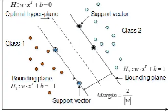
An SVM is a statistical machine learning technique that has been widely applied in data classification [13,19]. SVM completes the classification process by seeking the optimal hyper-plane with the maximal margin between the separate data classes. Taking two two-dimensional data sets as an example, the basic principle of the SVM classifier is illustrated in Fig. 1. The dashed line (H) is the optimal hyper-plane, which separates the two-class data points with the maximal margin, namely, the distance between H and the nearest data point in each class is maximal. These nearest data points are called as support vectors, while the two solid lines (H1 and H2) parallel to H are known as
bounding planes. The distance between H1 and H2 is the classification margin, which is equal to
2/‖w‖.The optimal hyper-plane parameters for the biggest margin can be transformed into a convex quadratic programming problem that can be solved more easily.
For linearly separable data, His found by solving the following equation:
𝑚𝑖𝑛1
2‖𝑤‖
2 subject to𝑦
𝑖(𝑤𝑇𝑋𝑖+ 𝑏) ≥ 1 (4)
For the non-linearly separable data, the data is mapped into a high-dimensional feature space by some non-linear mapping functions, called kernel functions. After data space transformation, the optimal hyper-plane can be built to separate the data linearly [19]. In this research, radial basis functions are used as the kernel functions.
Figure 1.Optimal separating hyper-plane for data classification
4 of 14
DAGSVM methods need a shorter training time [20-22]. Although DAGSVM needs the same training time as one-against-one, it has a shorter testing time. Therefore, the DAGSVM method is adopted in this project to identify the various operating status of the motor.
3. System Architecture and Implementation
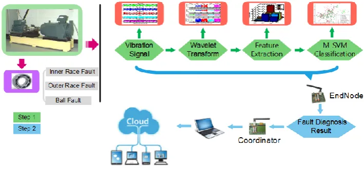
The architecture of the proposed machine fault diagnosis system using IIoT and IWSNs with on-sensor WT and multiclass support vector machine (M-SVM) is illustrated in Fig. 2. The system consists of a star topology IWSN with one coordinator and several sensor nodes, a computer working as the gateway, a cloud platform, and a management portal. ZigBee and a Jennic JN5139 sensor board and controller board are selected as the communication protocol and the hardware platform for the end nodes and the coordinator of the IWSN. The signal acquisition, WT fault feature extraction, and M-SVM fault diagnosis are completed on the IWSN end nodes, and then the fault diagnosis results are collected and transmitted through the coordinator and the gateway to the cloud platform for subsequent access by the management portal. The end nodes can switch to sleep mode between signal acquisition, fault feature extraction, and fault diagnosis stages to reduce node energy consumption and prolong the lifetime of IWSNs and IIoT. The details of the system are described below.
3.1. Machine Fault Signal
As introduced in section I, this project uses the vibration data of normal and faulty bearings provided by the Bearing Data Center at CWRU as the training and testing data for the proposed on-sensor fault diagnosis method. The test bed of CWRU is shown in the left part of Fig. 2. It consists of a 2 hp reliance electric motor, a torque transducer, and a dynamometer. The motor speed is 1797rpm. Rolling ball fault, inner race fault, and outer race fault with different fault diameters were separately seeded on the normal bearing using electro-discharge machining, and the vibration signal is collected using accelerometers and a 16 channel DAT recorder with 12 kHz sampling frequency.
Figure 2.The overall architecture of the proposed system
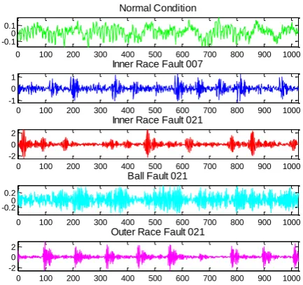
In this paper, five bearing working conditions, namely normal condition bearing (NOR), bearing with inner raceway fault of 0.007 inches in diameter (IR007), bearing with inner raceway fault of 0.021 inches in diameter (IR021), bearing with rolling ball fault of 0.021 inches in diameter (B021), and bearing with outer raceway fault of 0.021 inches in diameter (OR021), are selected for further fault diagnosis experiment.
5 of 14
Figure 3.The original vibration signal of the bearing with different conditions
3.2. Wavelet Transform Fault Feature Extraction
One wavelet transform method with low-memory requirements presented in [23] is selected for the resources-constrained IWSN nodes. The 2-level wavelet transform on bearing vibration signals with four popular used mother wavelets, namely Db97, Db53, Coiflet1, and Symlet2 wavelets, are computed to verify the feasibility of the proposed on-sensor WT fault feature extraction, and to compare the fault feature extraction effectiveness of the various mother wavelets. The selected four mother wavelets are shown in Fig. 4. The filter coefficients of Db97, Db53, Coiflet1, and Symlet2 wavelets are given in Table 1, Table 2, and Table 3.
Figure 4.Various mother wavelets
0 100 200 300 400 500 600 700 800 900 1000
-0.1 0 0.1
Normal Condition
0 100 200 300 400 500 600 700 800 900 1000
-1 0 1
Inner Race Fault 007
0 100 200 300 400 500 600 700 800 900 1000
-2 0 2
Inner Race Fault 021
0 100 200 300 400 500 600 700 800 900 1000
-0.20
0.2
Ball Fault 021
0 100 200 300 400 500 600 700 800 900 1000
-2 0 2
Outer Race Fault 021
Original Normal and Fault Vibration Signal
0 5 10 15 20
-2 -1 0 1
time
A
m
p
li
tu
d
e
Db97
0 5 10
-2 -1 0 1 2
time
A
m
p
li
tu
d
e
Db53
0 2 4 6
-2 0 2 4
time
A
m
p
li
tu
d
e
Coiflet1
0 1 2 3
-2 -1 0 1 2
time
A
m
p
li
tu
d
e
6 of 14
Table 1.The Filter Coefficients of Db97 Wavelet [23]
J analysis lowpassLj
analysis highpassHj
synthesis lowpassLj
synthesis highpassHj
-4 0.037828 0.037828
-3 -0.023849 0.064539 0.064539 -0.023849
-2 -0.110624 -0.040689 -0.040689 -0.110624
-1 0.377403 -0.418092 -0.418092 0.377403
0 0.852699 0.788486 0.788486 0.852699
1 0.377403 -0.418092 -0.418092 0.377403
2 -0.110624 -0.040689 -0.040689 -0.110624
3 -0.023849 0.064539 0.064539 -0.023849
4 0.037828 0.037828
Table 2. The Filter Coefficients of Db53 Wavelet [24]
J analysis lowpassLj
analysis highpassHj
synthesis lowpassLj
synthesis highpassHj
-2 -0.125 -0.125
-1 0.250 -0.500 0.500 -0.250
0 0.750 1.000 1.000 0.750
1 0.250 -0.500 0.500 -0.250
2 -0.125 -0.125
Table 3.The Filter Coefficients of Coiflet1 and Symlet2 Wavelet [25]
Wavelet coefficients
Wavelet
Symlet2 Coiflet1
h0 -0.1294095226 -0.0156557281 h1 0.2241438680 -0.0727326195 h2 0.8365163037 0.3848648469 h3 0.4829629131 0.4829629131
h4 0.3378976625
h5 -0.0727326195
g0 -0.4829629131 0.0727326195 g1 0.8365163037 0.3378976625 g2 -0.2241438680 -0.8525720202 g3 -0.1294095226 0.3848648469
g4 0.0727326195
g5 -0.0156557281
After the wavelet transform, the signal energies of the wavelet coefficients of each DWT level are calculated as the fault features to reduce fault feature set size because wavelet coefficients are still too large to be directly transmitted by the IWSNs as the fault features. The signal energy feature used in this paper is defined as follows:
2 2
0
1
( ) ( )
n
j j j
k
E + S t dt y k
=
=
=
(5)Where Sj(t) is the wavelet signal in decomposition level j, yj(k)is the kth wavelet coefficients in
7 of 14
wavelet coefficients is then used as the input of the M-SVM fault classifier which will be described in the next section.
3.3. M-SVM Fault Diagnosis
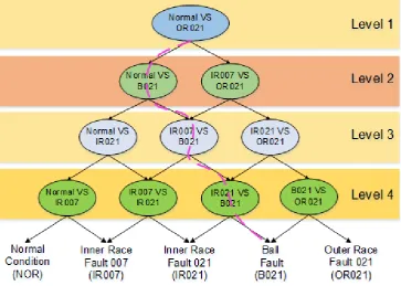
Due to its short training and testing time, DAGSVM is chosen as the multiclass fault classifier in this paper. The principle of a DAG for classifying five machine working conditions is shown in Fig.5. We can see that there are 5*(5-1)/2=10 internal nodes and 5 leaf nodes in Fig.5. Each internal node is a binary SVM classifier that has been trained by a distinct pair of machine working conditions, while each leaf node indicates one working condition. To evaluate a test data set, we start at the root node. The binary output of the root node, namely Normal VS OR021, is calculated first, the node is then exited via the left edge if the result does not indicate OR021; or the right edge if the binary output does not indicate Normal. The binary output of the next node (for example, Normal VS B021 in level 2 is then evaluated. By repeating this calculation and evaluation process at every level, we can travel down the DAG and finally reach a leaf node that indicates the predicted machine working condition. For a problem with N classes, N-1 decision nodes, one in each level, will be evaluated to complete the classification procedure. In this research, N is set as 5. The purple dotted line in Fig. 5 is one possible path taken through the DAG, representing the evaluation path.
Figure 5. The DAG for selecting the correct machine working condition out of five classes
4. Experimental Validation
8 of 14
4.2 WT Fault Feature Extraction
In this experiment, the feasibility of on-sensor fault feature extraction using WT is explored. The 2-level wavelet transforms with four different mother wavelets, namely Db97, Db53, Coiflet1 and Symlet2 wavelet, are conducted on IWSNs node to decompose vibration signals in the five conditions, namely NOR, IR007, IR021, B021, and OR021.
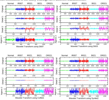
The vibration data used in this step are collected from the sensor nodes installed at the fan end of the motor housing. 1024 samples constitute a data set of one bearing condition, so the total number of samples is 5120. The original vibration signals and corresponding wavelet coefficients after 2-level DWT are shown as Fig. 6, where Detail 1 is the detail coefficients at 1st level, Detail 2 is the detail coefficients at 2nd level, and Approx 2 is the approximation coefficients at 2nd level. Although vibration signals amplitude rose significantly for a faulty bearing, it is still difficult to decide bearing working condition just by vibration signal amplitude. In addition, compared to the normal condition, the wavelet coefficients of the faulty bearings have different characteristics.
Figure 6. The 2-level DWT decomposition of the vibration signals under five bearing working conditions using four different mother wavelets
E1, E2, and E3, the energy of the corresponding wavelet coefficients of the testing data sets, are then calculated on the sensor node. Although the sum of energy of all the wavelet coefficients at all details and approximate parts is equal to the energy of the original vibration signal, the energy distribution at various frequency bands will change according to the bearing working condition. The normalized wavelet energy signals are shown in Fig. 7. It is easier to distinguish the different bearing working status by using the energy signals than using vibration amplitude.
0 500 1000 1500 2000 2500 3000 3500 4000 4500 5000 -2
0 2
Original
Normal IR007 IR021 B021 OR021
0 500 1000 1500 2000 2500
-4 -2 0 2 Detail 1
0 200 400 600 800 1000 1200
-4 -2 0 2 Detail 2
0 200 400 600 800 1000 1200
-0.5 0 0.5
Approx 2
Wavelet Transform using Db97
0 500 1000 1500 2000 2500 3000 3500 4000 4500 5000 -2
0 2
Original
Normal IR007 IR021 B021 OR021
0 500 1000 1500 2000 2500
-4 -2 0 2 Detail 1
0 200 400 600 800 1000 1200
-4 -2 0 2 Detail 2
0 200 400 600 800 1000 1200
-0.5 0 0.5
Approx 2
Wavelet Transform using Db53
0 500 1000 1500 2000 2500 3000 3500 4000 4500 5000 -2
0 2
Original
Normal IR007 IR021 B021 OR021
0 500 1000 1500 2000 2500
-4 -2 0 2 Detail 1
0 200 400 600 800 1000 1200
-4 -2 0 2 Detail 2
0 200 400 600 800 1000 1200
-0.5 0 0.5
Approx 2
Wavelet Transform using Coiflet1
0 500 1000 1500 2000 2500 3000 3500 4000 4500 5000 -2
0 2
Original
Normal IR007 IR021 B021 OR021
0 500 1000 1500 2000 2500
-4 -2 0 2 Detail 1
0 200 400 600 800 1000 1200
-4 -2 0 2 Detail 2
0 200 400 600 800 1000 1200
-0.5 0 0.5
Approx 2
9 of 14
Figure 7.The normalized energy of wavelet coefficients for vibration signals under five bearing working conditions using four different mother wavelets
4.2. M-SVM Fault Diagnosis
In this section, the feasibility of on-sensor multiclass fault diagnosis using DAGSVM is investigated. The vibration data from the bearing under the above mentioned five working conditions are used.
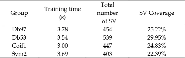
First, a total of 450 training data sets, 90 for each condition, are used to train the 10 SVM binary classifiers off-line. After training, the obtained M-SVM classifier parameters with different mother wavelets are given in Table 4. It can be seen that Coiflet1 (Coif1) wavelet needs the least training time, while Symlet2 (Sym2) has the smallest support vector number and potentially shortest calculation time in the on-line fault diagnosis procedure.
Table 4. M-SVM Classifier Parameters Using Different Wavelet
Group Training time (s)
Total number
of SV
SV Coverage
Db97 3.78 454 25.22%
Db53 3.54 539 29.95%
Coif1 3.00 447 24.83%
Sym2 3.69 403 22.39%
The training accuracies of M-SVM classifiers with different mother wavelets are given in Table 5. It can be seen that the total training accuracy of M-SVM classifiers with Coiflet1 and Symlet2 wavelet reach 98%, while the accuracy of Db97 and Db53 are 93% and 95%, respectively.
Second, the obtained parameters of the M-SVM classifiers are then embedded in the program on the sensor nodes. Then 140 data sets, 28 for each condition, were used for testing and verification on-line. 1 2 3 4 5 1 2 3 0 0.2 0.4 0.6 0.8 1
Energy Characteristics Extraction using Db97
E n e rg y A m p lit u d e IR007 IR021 B021 OR021 Normal Detail2 Detail1 Approx2 1 2 3 4 5 1 2 3 0 0.2 0.4 0.6 0.8
Energy Characteristics Extraction using Db53
E n e rg y A m p lit u d e IR007 IR021 B021 OR021 Normal Detail2 Detail1 Approx2 1 2 3 4 5 1 2 3 0 0.2 0.4 0.6 0.8 1
Energy Characteristics Extraction using Coiflet1
E n e rg y A m p lit u d e IR007 IR021 B021 OR021 Normal Detial2 Detial1 Approx2 1 2 3 4 5
1 2 3
0 0.2 0.4 0.6 0.8 1
Energy Characteristics Extraction using Symlet2
E n e rg y A m p lit u d e IR007 IR021 B021 OR021 Normal
10 of 14
Table 5. The Training Accuracy of M-SVM Classifiers with Different Mother Wavelets
Fault Type IR007 IR021 B021 OR021 NOR Total Number of
Training Samples 90 90 90 90 90 450
Training Accuracy
(%)
Db97 95.56 84.45 96.67 90.00 100 93.33 Db53 98.89 91.11 97.78 93.33 100 96.22 Coif1 97.78 98.89 100 97.78 100 98.89
Sym2 95.56 100 94.45 100 100 98.00
The testing accuracy of M-SVM classifiers with different mother wavelets is given in Table 6. The training accuracy of SVM classifiers with all of the four mother wavelets exceeds 90%. The M-SVM classifier using Symlet2 wavelet gives the highest accuracy, which reaches 99.29%, while Coiflet1 wavelet has an accuracy of 98.57%.
Table 6.The Testing Accuracy of M-SVM Classifiers Using Different Wavelet
Wavelet Db97 Db53 Coif1 Sym2
Number of Test Samples 28*5 28*5 28*5 28*5 Testing Accuracy(%) 96.43 92.96 98.57 99.29
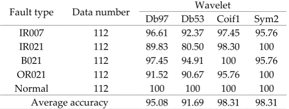
Third, 560 data sets from another set of vibration data are used to test the performance of the obtained M-SVM classifier models again. The results are given in Table 7. It can be seen that the classification accuracy of Coiflet1 and Symlet2 wavelet reaches 98.31%, and are better than the results of Db97 and Db53 wavelet.
Table 7. The Testing Accuracy of M-SVM Classifier by Another Data Set
Fault type Data number Wavelet
Db97 Db53 Coif1 Sym2 IR007 112 96.61 92.37 97.45 95.76
IR021 112 89.83 80.50 98.30 100
B021 112 97.45 94.91 100 95.76
OR021 112 91.52 90.67 95.76 100
Normal 112 100 100 100 100
Average accuracy 95.08 91.69 98.31 98.31
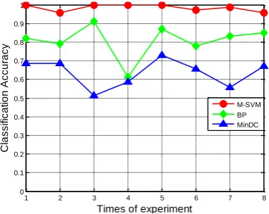
Fourthly, we randomly divide the 560 sets of data into 8 groups. Each group includes 70 data sets, 14 for each condition. These data are used to verify the overall classification effect of the obtained M-SVM classifier with different mother wavelets again. The results are shown in Fig.8. Compared with Db97 and Db53 wavelet, Coiflet1 and Symlet2 wavelet have higher overall classification accuracy (98.31%) and less fluctuation.
11 of 14
Figure 8.Comparison of fault diagnosis classification accuracy using different wavelet
Figure 9.Comparison of the classification accuracy of the proposed approach with neural network and minimum distance methods
4.3. Payload Transmission Data and Node Energy Consumption
In this section, the transmission data and node energy consumption for data transmitted after on-sensor WT fault feature extraction and SVM fault diagnosis and for raw data transmission are tested and compared by a series of experiments.
1) Payload transmission data: For raw data transmission mode, the IWSN end node should send 8192 bytes to the coordinator for 1024 samples. For on-sensor WT fault feature extraction and SVM fault diagnosis mode, the end node only needs to transmit the fault diagnosis result, so the payload transmission data decrease from 8192 to 4 bytes, i.e., a 99.95% reduction.
2) Node Energy Consumption: When a 16-MHz system clock is used, the typical current consumption of JN5139 CPU processing status is 7.57 mA. The calculating time for on-sensor WT fault feature extraction using Symlet2 mother wavelet and on-sensor DAGSVM multiclass fault diagnosis is around 2.12 s, so the energy consumption for the proposed on-sensor fault diagnosis approach is given as
𝐸𝑜𝑛−𝑠𝑒𝑛𝑠𝑜𝑟𝑑𝑖𝑎𝑔= 2.353𝑉 × 7.57𝑚𝐴 × 2.12𝑠 = 37.8 𝑚𝐽 (6)
Typical current consumption of JN5139 for wireless data transmitting is 38mA. The time for transmitting 8192 bytes raw data is about 0.47 s, the node voltage in this experiment is about 2.353 V, so the energy consumption for raw data transmission is
𝐸𝑟𝑎𝑤𝑑𝑎𝑡𝑎𝑡𝑟𝑎𝑛𝑠= 2.353𝑉 × 38𝑚𝐴 × 0.47𝑠 = 42.0 𝑚𝐽 (7)
1 2 3 4 5 6 7 8
0.6 0.65 0.7 0.75 0.8 0.85 0.9 0.95 1
Times of experiment
C
la
s
s
if
ic
a
ti
o
n
A
c
c
u
ra
c
y
Fault Diagnosis Performance of Differrent Classification Method
Coif1 Db97 Db53 Sym2
1 2 3 4 5 6 7 8
0 0.1 0.2 0.3 0.4 0.5 0.6 0.7 0.8 0.9 1
Times of experiment
C
la
s
s
if
ic
a
ti
o
n
A
c
c
u
ra
c
y
Fault Fiagnosis Accuracy using Differrent Classification Method
12 of 14
Compared with raw data direct transmission, the on-sensor fault diagnosis method using Symlet2 WT and DAGSVM reduces energy by 10%, 4.2 mJ.
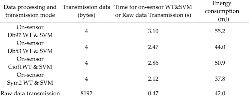
The details of payload data transmission and node energy consumption for raw data transmission and on-sensor fault diagnosis are given in Table 8. It can be seen that the energy consumption of on-sensor fault diagnosis depends on the calculation time and complexity of the selected algorithm. The energy consumption for on-sensor fault diagnosis with Db53 WT and SVM is similar to the energy utilization for raw data transmission, while the energy consumption of on-sensor fault diagnosis with Ciof1 WT or Db97 WT and SVM is higher than the energy utilization of raw data transmission
Table 8. Comparison of Transmission Data and Energy Consumption of Raw Data Transmission and On-sensor Fault Diagnosis
Data processing and transmission mode
Transmission data (bytes)
Time for on-sensor WT&SVM or Raw data Transmission (s)
Energy consumption
(mJ) On-sensor
Db97 WT & SVM 4 3.10 55.2
On-sensor
Db53 WT & SVM 4 2.47 44.0
On-sensor
Ciof1WT & SVM 4 2.86 50.9
On-sensor
Sym2 WT & SVM 4 2.12 37.8
Raw data transmission 8192 0.47 42.0
5. Conclusions
In this paper, we proposed a novel machine fault diagnosis method, which uses IIoT and IWSNs with on-sensor fault feature extraction by wavelet transform and on-sensor fault diagnosis by M-SVM to reduce the payload transmission data in IWSN. Four popular mother wavelets, namely Db97, Db53, Coiflet1, and Symlet2 wavelet, and DAGSVM are selected and implemented on the IWSN sensor node.
The feasibility and effectiveness of the presented approach have been demonstrated by a set of experiments using the bearing vibration data obtained from the Bearing Data Center at CWRU. Testing results show the following.
1) Compared with raw data transmission, the proposed on-sensor fault diagnosis method can reduce the payload transmission data by 99.95%, and reduce the node energy consumption by about 10%;
2) The fault diagnosis accuracy of the proposed method with all the four mother wavelets exceeds 91%, while the accuracy by Coiflet1 and Symlet2 wavelet reaches 98%;
3) The accuracy of the presented on-sensor approach with Coiflet1 wavelet is 15% and 30% higher than the accuracy of ANN and minimum distance methods.
The energy consumption results show that small energy savings can be made, of the order of 10% by using on-sensor computation. However, the relatively small savings suggest that there is still scope for improved performance by reducing the energy cost of on-sensor processing, using more energy efficient computation architectures such as FPGAs. Su, for example, has shown power savings of 90% for on-sensor computation by using low power FPGAs [25].
13 of 14
Bergmann; Visualization, Liqun Hou, Junteng Hao and Yongguang Ma; Writing – original draft, Liqun Hou, Junteng Hao and Yongguang Ma; Writing – review & editing, Neil Bergmann.
Funding: This work was supported by the Natural Science Foundation of Hebei Province, China (Grant No. F2016502104), the Scientific Research Foundation for the Returned Overseas Chinese Scholars, The Ministry of Education of the People's Republic of China, and the Fundamental Research Funds for the Central Universities of China.
Conflicts of Interest: The authors declare no conflict of interest.
References
1. Tavner, P. Review of condition monitoring of rotating electrical machines. IET Electric Power Applications
2008, 2, 215-247, doi:10.1049/iet-epa:20070280.
2. Da Xu, L.; He, W.; Li, S. Internet of things in industries: A survey. IEEE Transactions on industrial informatics
2014, 10, 2233-2243, doi:10.1109/TII.2014.2300753.
3. Farné, S.; Bassi, E.; Benzi, F.; Compagnoni, F. IIoT based efficiency monitoring of a Gantry robot. In Proceedings of IEEE 14th International Conference on Industrial Informatics (INDIN), Poitiers, France; pp. 714-719.
4. Şen, M.; Kul, B. IoT-based wireless induction motor monitoring. In Proceedings of XXVI International Scientific Conference Electronics, Sozopol, Bulgaria; pp. 1-5.
5. Sheng, Z.; Mahapatra, C.; Zhu, C.; Leung, V. Recent advances in industrial wireless sensor networks towards efficient management in IoT. IEEE access 2015, 3, 622-637, doi:10.1109/ACCESS.2015.2435000. 6. Wan, J.; Tang, S.; Shu, Z.; Li, D.; Wang, S.; Imran, M.; Vasilakos, A.V. Software-defined industrial internet
of things in the context of industry 4.0. IEEE Sensors Journal 2016, 16, 7373-7380, doi:10.1109/JSEN.2016.2565621.
7. Bergmann, N.W.; Hou, L.-Q. Energy Efficient Machine Condition Monitoring Using Wireless Sensor Networks. In Proceedings of International Conference on Wireless Communication and Sensor Network (WCSN),, Wuhan, China; pp. 285-290.
8. Wang, K.; Wang, Y.; Sun, Y.; Guo, S.; Wu, J. Green industrial internet of things architecture: An energy-efficient perspective. IEEE Communications Magazine 2016, 54, 48-54, doi:10.1109/MCOM.2016.1600399CM. 9. Hou, L.; Bergmann, N.W. Induction motor fault diagnosis using industrial wireless sensor networks and Dempster-Shafer classifier fusion. In Proceedings of 37th IEEE Annual Conference on Industrial Electronics Society (IECON 2011), Melbourne, Australia; pp. 2992-2997.
10. Hou, L.; Bergmann, N.W. Novel industrial wireless sensor networks for machine condition monitoring and fault diagnosis. IEEE Transactions on Instrumentation 2012, 61, 2787-2798, doi:10.1109/TIM.2012.2200817. 11. Neuzil, J.; Kreibich, O.; Smid, R. A distributed fault detection system based on IWSN for machine condition
monitoring. IEEE Transactions on Industrial Informatics 2014, 10, 1118-1123, doi:10.1109/TII.2013.2290432. 12. Hou, L.; Yang, L. Machine fault diagnosis using industrial wireless sensor networks and on-sensor wavelet
transform. In Proceedings of 43rd Annual Conference of the IEEE Industrial Electronics Society (IECON 2017), Beijing, China; pp. 6045-6050.
13. Jegadeeshwaran, R.; Sugumaran, V. Fault diagnosis of automobile hydraulic brake system using statistical features and support vector machines. Mechanical Systems and Signal Processing 2015, 52, 436-446, doi:0.1016/j.ymssp.2014.08.007.
14. Albrecht, P.; Appiarius, J.; McCoy, R.; Owen, E.; Sharma, D. Assessment of the reliability of motors in utility applications-Updated. IEEE Transactions on Energy conversion 1986, 10.1109/TEC.1986.4765668, 39-46, doi:10.1109/TEC.1986.4765668.
15. Group, I.M.R.W. Report of large motor reliability survey of industrial and commercial installations, Part I.
IEEE Trans. Ind. App.1985, 21, 853-864, doi:10.1109/TIA.1985.349532.
16. University, C.W.R. Case Western Reserve University Bearing Data Center. Availabe online: http://csegroups.case.edu/bearingdatacenter/home (accessed on 15 October, 2018).
14 of 14
18. Rafiee, J.; Tse, P.; Harifi, A.; Sadeghi, M. A novel technique for selecting mother wavelet function using an intelligent fault diagnosis system. Expert Systems with Applications 2009, 36, 4862-4875, doi:10.1016/j.eswa.2008.05.052.
19. Konar, P.; Chattopadhyay, P. Bearing fault detection of induction motor using wavelet and Support Vector Machines (SVMs). Applied Soft Computing 2011, 11, 4203-4211, doi:10.1016/j.asoc.2011.03.014.
20. Deng, S.; Lin, S.-Y.; Chang, W.-L. Application of multiclass support vector machines for fault diagnosis of field air defense gun. Expert Systems with Applications 2011, 38, 6007-6013, doi:10.1016/j.eswa.2010.11.020. 21. Huang, J.; Hu, X.; Geng, X. An intelligent fault diagnosis method of high voltage circuit breaker based on
improved EMD energy entropy and multi-class support vector machine. Electric Power Systems Research
2011, 81, 400-407, doi:10.1016/j.epsr.2010.10.029.
22. Pai, P.-F.; Chen, S.-Y.; Huang, C.-W.; Chang, Y.-H. Analyzing foreign exchange rates by rough set theory and directed acyclic graph support vector machines. Expert systems with applications 2010, 37, 5993-5998, doi:10.1016/j.eswa.2010.02.006.
23. Rein, S.; Reisslein, M.; Tutorials. Low-memory wavelet transforms for wireless sensor networks: A tutorial.
IEEE Communications Surveys & Tutorials 2011, 13, 291-307, doi:10.1109/SURV.2011.100110.00059.
24. Christopoulos, C.; Skodras, A.; Ebrahimi, T. The JPEG2000 still image coding system: an overview. IEEE transactions on consumer electronic 2000, 46, 1103-1127, doi:10.1109/30.920468.
![Table 2. The Filter Coefficients of Db53 Wavelet [24]](https://thumb-us.123doks.com/thumbv2/123dok_us/8080315.1348233/6.595.136.461.312.408/table-filter-coefficients-db-wavelet.webp)