R E S E A R C H A R T I C L E
Cokriging for enhanced spatial interpolation of rainfall in two
Australian catchments
Sajal Kumar Adhikary
1,2|
Nitin Muttil
1,2|
Abdullah Gokhan Yilmaz
31
College of Engineering and Science, Victoria University, P.O. Box 14428, Melbourne, Victoria 8001, Australia
2
Institute for Sustainability and Innovation, Victoria University, P.O. Box 14428, Melbourne, Victoria 8001, Australia
3
College of Engineering, University of Sharjah, P.O. Box 27272, Sharjah, United Arab Emirates
Correspondence
Sajal Kumar Adhikary, College of Engineering and Science, Victoria University, Footscray Park Campus, P.O. Box 14428, Melbourne, Victoria 8001, Australia.
Email: [email protected]
Abstract
Rainfall data in continuous space provide an essential input for most hydrological and water
resources planning studies. Spatial distribution of rainfall is usually estimated using ground‐based
point rainfall data from sparsely positioned rain‐gauge stations in a rain‐gauge network. Kriging
has become a widely used interpolation method to estimate the spatial distribution of climate
var-iables including rainfall. The objective of this study is to evaluate three geostatistical (ordinary
kriging [OK], ordinary cokriging [OCK], kriging with an external drift [KED]), and two deterministic
(inverse distance weighting, radial basis function) interpolation methods for enhanced spatial
interpolation of monthly rainfall in the Middle Yarra River catchment and the Ovens River
catch-ment in Victoria, Australia. Historical rainfall records from existing rain‐gauge stations of the
catchments during 1980–2012 period are used for the analysis. A digital elevation model of each
catchment is used as the supplementary information in addition to rainfall for the OCK and
kriging with an external drift methods. The prediction performance of the adopted interpolation
methods is assessed through cross‐validation. Results indicate that the geostatistical methods
outperform the deterministic methods for spatial interpolation of rainfall. Results also indicate
that among the geostatistical methods, the OCK method is found to be the best interpolator
for estimating spatial rainfall distribution in both the catchments with the lowest prediction error
between the observed and estimated monthly rainfall. Thus, this study demonstrates that the use
of elevation as an auxiliary variable in addition to rainfall data in the geostatistical framework can
significantly enhance the estimation of rainfall over a catchment.
K E Y W O R D S
cross‐variogram model, digital elevation model, kriging with an external drift, ordinary cokriging,
positive‐definite condition, variogram model
1
|I N T R O D U C T I O N
Rainfall data provide an essential input for many hydrological
investiga-tions and modelling tasks. Accuracy of various hydrological analyses such
as water budget analysis, flood modelling, climate change studies, drought
management, irrigation scheduling, and water management greatly
depends on the correct estimation of the spatial distribution of rainfall
(Delbari, Afrasiab, & Jahani, 2013; Moral, 2010). This usually requires a
dense rain‐gauge network with a large number of stations (Adhikary,
Muttil, & Yilmaz, 2016a). However, the rain‐gauge network is often sparse
in the field because the number of stations in a network is often restricted
by economic, logistics, and geological factors (Goovaerts, 2000). As a result,
point rainfall data are generally accessible from a limited number of
stations. These limitations increase the need for using suitable spatial
esti-mation methods to obtain the spatial distribution of rainfall and generate
rainfall map from the point rainfall values. Moreover, the network is often
not deployed on a regular grid and rainfall data may not be available in the
target location where it is most required (Adhikary et al., 2016a). In such
cases, spatial interpolation plays a vital role to simulate rainfall in areas with
no stations based on the observed rainfall values in the surrounding areas.
This is an open access article under the terms of the Creative Commons Attribution‐NonCommercial‐NoDerivs License, which permits use and distribution in any medium, provided the original work is properly cited, the use is non‐commercial and no modifications or adaptations are made.
© 2017 The Authors. Hydrological Processes Published by John Wiley & Sons Ltd. DOI: 10.1002/hyp.11163
Several interpolation methods have been frequently employed to
interpolate rainfall data from rain‐gauge stations and produce the spatial
distribution of rainfall over a catchment. Examples of such methods range
from simple conventional (e.g., Thiessen polygons [Thiessen, 1911],
isohyet mapping [ASCE, 1996], simple trend surface interpolation
[Gittins, 1968]), and deterministic methods (i.e., inverse distance
weighting (IDW; ASCE, 1996), radial basis function (RBF; Di Piazza, Conti,
Noto, Viola, & Loggia, 2011) to complex stochastic or geostatistical
methods (i.e., ordinary kriging [OK], ordinary cokriging [OCK] and kriging
with an external drift [KED; Goovaerts, 2000]). Although the
conven-tional and deterministic methods have been improved over time, their
limitations continue to exist. These limitations have been described
elab-orately in Goovaerts (2000) and Teegavarapu and Chandramouli (2005).
Geostatistical methods have been shown superior to the
conven-tional and deterministic methods for spatial interpolation of rainfall
(Goovaerts, 1997; Isaaks & Srivastava, 1989). Several studies have
reported that rainfall is generally characterised by a significant spatial
variation (e.g., Delbari et al., 2013; Lloyd, 2005). This suggests that
inter-polation methods, which are explicitly able to incorporate the spatial
variability of rainfall into the estimation process should be employed.
In view of that, kriging has become the most widely used geostatistical
method for spatial interpolation of rainfall. The ability of kriging to
produce spatial predictions of rainfall has been distinguished in many
studies (e.g., Adhikary et al., 2016a; Goovaerts, 2000; Jeffrey, Carter,
Moodie, & Beswick, 2001; Lloyd, 2005; Moral, 2010; Yang, Xie, Liu, Ji,
& Wang, 2015). The major advantage of kriging is that it takes into
account the spatial correlation between data points and provides
unbiased estimates with a minimum variance. The spatial variability in
kriging is quantified by the variogram model that defines the degree
of spatial correlation between the data points (Webster & Oliver, 2007).
Another key advantage of kriging over the conventional and
deter-ministic methods is that while providing a measure of prediction
stan-dard error (also called kriging variance), it is capable of complementing
the sparsely sampled primary variable, such as rainfall by the correlated
densely sampled secondary variable, such as elevation to improve the
estimation accuracy of primary variable (Goovaerts, 2000; Hevesi,
Istok, & Flint, 1992). This multivariate extension of kriging is referred
to as the cokriging method. The standard form of cokriging is the
OCK method, which usually reduces the prediction error variance and
specifically outperforms kriging method if the secondary variable (i.e.,
elevation) is highly correlated (correlation coefficient higher than .75)
with the primary variable (i.e., rainfall) and is known at many more
points (Goovaerts, 2000). The KED is another commonly applied
cokriging method, which can incorporate the exhaustive secondary
var-iable (i.e., elevation) to give an enhanced estimation of rainfall when
dealing with a low‐density rain‐gauge network. Thus, cokriging
includ-ing the OCK and KED methods has been the increasinclud-ing preferred
geostatistical methods all over the word. As highlighted by Goovaerts
(2000) and Feki, Slimani, and Cudennec (2012), rainfall and elevation
tend to be related because of the orographic influence of mountainous
topography. Therefore, topographic information such as the digital
ele-vation model (DEM) can be used as a convenient and valuable source of
secondary data for the OCK and KED methods. The efficacy of
incorpo-rating elevation into the interpolation procedure for enhanced
estima-tion of rainfall has been highlighted in many studies across the world
(e.g., Di Piazza et al., 2011; Feki et al., 2012; Hevesi et al., 1992; Lloyd,
2005; Martínez‐cob, 1996; Moral, 2010; Phillips, Dolph, & Marks,
1992; Subyani & Al‐Dakheel, 2009).
A wide variety of spatial interpolation methods have been
devel-oped for the interpolation of spatially distributed point rainfall values.
However, it is often challenging to distinguish the best interpolation
method to estimate the spatial distribution of rainfall for a particular
catchment or study area. The reason is that the performance of an
interpolation method depends on a number of factors such as
catch-ment size and characteristics, sampling density, sample spatial
distribu-tion, sample clustering, surface type, data variance, grid size or
resolution, quality of auxiliary information to be used as well as the
interactions among these factors. Moreover, it is unclear how the
afore-mentioned factors affect the performance of the spatial interpolation
methods (Dirks, Hay, Stow, & Harris, 1998; Li & Heap, 2011). Hence,
the best interpolation method for a particular study area is usually
established through the comparative assessment of different
interpola-tion methods (e.g., Delbari et al., 2013; Dirks et al., 1998; Goovaerts,
2000; Hsieh, Cheng, Liou, Chou, & Siao, 2006; Mair & Fares, 2011;
Moral, 2010). The comparison among different interpolation methods
is made through a validation procedure. The interpolation method that
provides better results with lower bias and higher accuracy in rainfall
estimation is identified as the best interpolation method.
In the past, many studies have been devoted to the comparison
and evaluation of different deterministic and geostatistical
interpola-tion methods in a range of different regions and climates around the
world. Dirks et al. (1998) compared four spatial interpolation methods
using rainfall data from a network of 13 rain‐gauges in Norfolk Island
concluding that kriging provided no substantial improvement over
any of the simpler Thiessen polygon (TP), IDW, or areal‐mean
methods. Goovaerts (2000) employed three multivariate geostatistical
methods (OCK, KED, simple kriging with varying local means [SKVM]),
which incorporate a DEM as secondary variable and three univariate
methods (OK, TP, and IDW) that do not take into account the elevation
for spatial prediction of monthly and annual rainfall data available at 36
rain‐gauge stations. The comparison among these methods indicated
that the three multivariate geostatistical methods gave the lowest
errors in rainfall estimation. Martínez‐cob (1996) compared OK, OCK,
and modified residual kriging to interpolate annual rainfall and
evapo-transpiration in Aragón, Spain. The results indicated that OCK was
superior for rainfall estimation, reducing estimation error by 18.7%
and 24.3% compared with OK and modified residual kriging,
respec-tively. Hsieh et al. (2006) evaluated OK and IDW methods using daily
rainfall records from 20 rain‐gauges to estimate the spatial distribution
of rainfall in the Shih‐Men Watershed in Taiwan. The results
demon-strated that IDW produced more reasonable representations than
OK. Moral (2010) compared three univariate kriging (simple kriging
[SK], universal kriging, and OK) with three multivariate kriging methods
(OCK, SKVM, and regression kriging) to interpolate monthly and
annual rainfall data from 136 rain‐gauges in Extremadura region of
Spain. The results showed that multivariate kriging outperformed
uni-variate kriging and among multiuni-variate kriging, SKVM and regression
kriging performed better than OCK.
Ly, Charles, and Degré (2011) used IDW, TP, and several kriging
The results indicated that integrating elevation into KED and OCK did
not provide improvement in the interpolation accuracy for daily rainfall
estimation. OK and IDW were considered to be the suitable methods
as they gave the smallest error for almost all cases. Mair and Fares
(2011) compared TP, IDW, OK, linear regression, SKVM to estimate
seasonal rainfall in a mountainous watershed concluding that OK
pro-vided the lowest error for nearly all cases. They also found that
incor-porating elevation did not improve the prediction accuracy over OK for
the correlation between rainfall and elevation lower than 0.82. Delbari
et al. (2013) used two univariate methods (IDW and OK), and four
mul-tivariate methods (OCK, KED, SKVM, and linear regression) for
map-ping monthly and annual rainfall over the Golestan Province in Iran.
They reported that KED and OK outperformed all other methods in
terms of root mean square error (RMSE). Jeffrey et al. (2001) derived a
comprehensive archive of Australian rainfall and climate data using a
thin plate smoothing spline to interpolate daily climate variables and
OK to interpolate daily and monthly rainfall. The aforementioned
studies on spatial interpolation of rainfall indicate that each method
has its advantages and disadvantages and thus performs in a dissimilar
way for different regions. There is no single interpolation method that
can work well everywhere (Daly, 2006). Therefore, the best interpolator
for a particular study area or catchment should essentially be achieved
through the comparative assessment of different interpolation methods.
To date, many studies have been conducted on spatial
interpola-tion of rainfall at a regional and nainterpola-tional scale in Australia (Gyasi‐Agyei,
2016; Hancock & Hutchinson, 2006; Hutchinson, 1995; Jeffrey et al.,
2001; Johnson et al., 2016; Jones, Wang, & Fawcett, 2009; Li & Shao,
2010; Woldemeskel, Sivakumar, & Sharma, 2013; Yang et al., 2015).
However, none of these studies was conducted at a local or catchment
scale. Likewise, elevation and rainfall relations locally have been
rela-tively little studied in Australia and no such studies have been
under-taken specifically within the Yarra River catchment and the Ovens
River catchment in Victoria, Australia. Sharma and Shakya (2006)
highlighted that any analysis of hydroclimatic variables should be
car-ried out at the local scale rather than at a large or global scale because
of the variations of hydroclimatic situations from one region to
another. Therefore, the main aim of this study is to assess if relatively
more complex geostatistical interpolation methods that take into
account the elevation and rainfall relation provide any benefits over
simpler methods for enhanced estimation of rainfall within the Yarra
River catchment and the Ovens River catchment in Victoria, Australia.
The specific focus is to evaluate the effectiveness of the cokriging
methods including OCK and KED that make use of elevation as a
sec-ondary variable over those methods including OK, IDW, and RBF that
do not make use of such information to estimate the spatial
distribu-tion of rainfall within the catchment. This study is expected to provide
an important contribution towards the enhanced estimation of rainfall
in the aforementioned two Australian catchments using the cokriging
methods by incorporating elevation as an auxiliary variable in addition
to rainfall data. One specific contribution of this paper is in explaining
how rainfall varies with elevation from catchment to catchment.
The Yarra River catchment and the Ovens River catchment in
Victoria are selected for this study because they are two important
water resources catchments in Australia in terms of water supply and
agricultural production (Adhikary, Yilmaz, & Muttil, 2015; EPA Victoria,
2003; Schreider, Jakeman, Pittock, & Whetton, 1996; Yu, Cartwright,
Braden, & de Bree, 2013). The Yarra River catchment is a major source
of water for more than one third of Victoria's population in Australia
(Barua, Muttil, Ng, & Perera, 2012). Although the catchment is not
large with respect to other Australian catchments, it produces the
fourth highest water yield per hectare of the catchment in Victoria
(Adhikary et al., 2015). There are seven storage reservoirs in the
catch-ment that supports about 70% of drinking water supply in Melbourne
city (Barua et al., 2012). The Ovens River catchment is another
impor-tant source of water in northeast Victoria, which forms a part of the
Murray‐Darling basin (Yu et al., 2013). The Ovens River is
consid-ered one of the most important tributaries of the Murray‐Darling
Basin due to the availability of sufficient volume of water with
accept-able quality and its good ecological condition. The average annual flow
of the river constitutes approximately 7.3% of the total flow of the state
of Victoria (Schreider et al., 1996). The catchment contributes
approxi-mately 14% of Murray‐Darling basin flows in spite of its relatively small
catchment area of less than 1% of the total Murray‐Darling basin area
(EPA Victoria, 2003; Yu et al., 2013). Thus, both the catchments have
sig-nificant contribution towards the sustainable development of Victoria's
economy. However, high rainfall variation and diverse water use
activities in these catchments has complicated the water management
tasks, which has further created strong burden on the water managers
and policy makers for effective water resources management. Therefore,
enhanced estimation of rainfall and its spatial distribution is important,
which could be beneficial for effective water supply and demand
man-agement, and sustainable agricultural planning in both the catchments.
The rest of the paper is arranged as follows. First, a brief
descrip-tion of the study area and data used are presented, which is followed
by the detailed description of the methodology adopted in this study.
The results are summarized next, and finally, the conclusions drawn
from this study are presented.
2
|S T U D Y A R E A A N D D A T A U S E D
2.1
|The study area
This study considers two catchments in Victoria as the case study area,
which includes the Middle Yarra River catchment and Ovens River
catchment in south‐eastern Australia. Figure 1 shows the approximate
location of the case study area. The Yarra River catchment is located in
northeast of Melbourne covering an area of 4,044 km2. The water
resources management is an important and multifaceted issue in the
Yarra River catchment because of its wide range of water uses as well
as its downstream user requirements and environmental flow
provi-sions (Barua et al., 2012). The catchment significantly contributes to
the water supply in Melbourne and has been playing an important role
in the way Melbourne has been developed and grown (Adhikary et al.,
2015). The Yarra River catchment consists of three distinctive sub‐
catchments including Upper, Middle, and Lower Yarra segments based
on different land use activities (Barua et al., 2012). This study
concen-trates on the Middle segment of the Yarra River catchment, which
forms part of the case study area in Figure 1. The Upper Yarra segment
includes mainly the forested and mountainous areas with minimum
catchment for Melbourne and has been reserved for more than
100 years for water supply purposes. The MiddleYarra segment, starting
from the Warburton Gorge to Warrandyte Gorge, is notable as the only
part of the catchment with an extensive flood plain, which is mainly used
for agricultural activities. The Lower Yarra segment of the catchment,
which is located downstream of Warrandyte, is mainly characterized
by the urbanized floodplain areas of Melbourne city (Adhikary, Muttil,
& Yilmaz, 2016b). Most of the land along rivers and creeks in the middle
and lower segments has been cleared for the agricultural or urban
development (Barua et al., 2012; Melbourne Water, 2015).
Rainfall varies significantly through different segments of the Yarra
River catchment. The mean annual rainfall varies across the catchment
from 600 mm in the Lower Yarra segment to 1,100 mm in the Upper
Yarra segment (Daly et al., 2013). The Middle Yarra segment (part of
the case study area in Figure 1) covers an area of 1,511 km2and consists
of three storage reservoirs. Decreasing rainfall patterns in the catchment
will reduce the streamflows, which in turn will lead to the reduction in
reservoir inflows and hence impact the overall water availability in the
catchment. Moreover, the reduced streamflows may cause increased risk
of bushfires. Conversely, increasing rainfall patterns and the occurrence
of extreme rainfall events (as reported in Yilmaz and Perera [2014] and
Yilmaz, Hossain, and Perera [2014]) will result in excess amount of
streamflows that may cause flash floods in the urbanized lower segment
and makes it vulnerable and risk‐prone. The urbanized lower part of the
catchment is also dependent on the water supply from the storage
reservoirs mainly located in the middle and upper segments of the
catchment (Adhikary et al., 2015). Therefore, accurate spatial distribution
of rainfall in the middle and upper segments of the catchment could be
useful for accurate estimation of future streamflows for optimal reservoir
operation and effective flood control in the urbanized lower part.
The Ovens River catchment in northeast Victoria is also
consid-ered as a part of the case study area in this study, which is shown in
Figure 1. The catchment covers an area of 7,813 km2 (Yu et al.,
2013), which extends from the Great Dividing Range in the south
to the Murray River in the north, with the Yarrawonga Weir forming
the downstream boundary. It is considered to be one of the least
modified catchments within the Murray‐Darling basin. The catchment
contributes approximately 14% to the average flows of the Murray
River in spite of its relatively small size (0.75 percent of the total
Murray‐Darling Basin area; EPA Victoria, 2003; Yu et al., 2013). The
Ovens River is the main river in the catchment, which originates on
the northern edges of the Victorian Alps and flows in a north‐
west-erly direction until its junction with the Murray River near Lake
Mulwala. The riverine plains and alluvial flats are primarily cleared
for agricultural use, while the hills and mountains are covered by
forests with native plant species (Yu et al., 2013). Total average water
use in the catchment is about 30,000 million litres per year, 64% of
which is diverted from the Ovens River and its tributaries. A major
part of this water use is irrigation, which constitutes more than
16,000 million litres annually (Schreider et al., 1996). The river itself
provides natural conditions suitable for many significant native fish
species, particularly the endangered Murray Cod (EPA Victoria,
2003). Thus, the catchment is considered to be important, not only
at a regional scale, but also at the national scale in terms of its water
supply volume for domestic and agricultural production, and high
environmental value.
The climate of the Ovens River catchment varies considerably
with topography and elevation (Yu et al., 2013). The average annual
rainfall varies from 1,127 mm in the Alpine region at Bright to
occurring in winter months (Yu et al., 2013). Approximately 45% of the
annual rainfall occurs during the winter (June to September) whereas
the summer is warm and dry. Winter snowfalls are common at
alti-tudes above 1,000 m (EPA Victoria, 2003). Therefore, enhanced
esti-mation of rainfall and its spatial distribution could be useful for the
effective management of water supply and agricultural activities in
the catchment.
2.2
|Data used
In this study, historical rainfall data from existing rain‐gauge stations in
the Middle Yarra River catchment and the Ovens River catchment
(Figure 1) for 1980–2012 period are considered. There are 19 rain‐
gauge stations in the Middle Yarra River catchment, whereas the
Ovens River catchment includes 42 rain‐gauge stations operated by
the Australian Bureau of Meteorology. Daily rainfall data are collected
from the Scientific Information for Land Owners climate database
(http://www.longpaddock.qld.gov.au/silo/) and compiled to generate
monthly and annual rainfall, which are then used for the analysis.
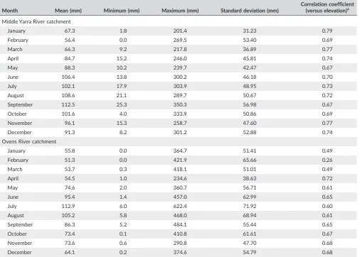
Sum-mary statistics of monthly rainfall data are given in Table 1. The annual
average rainfall in the Middle Yarra River catchment for the
aforemen-tioned period varies from 710 mm to 1422 mm with a mean value of
1082 mm. The southern and south‐eastern part experiences the
highest rainfall, whereas the lowest rainfall occurs in the north‐western
part in the study area. September is the wettest month (rainfall amount
equals to 112.5 mm) with the highest variation in rainfall. The driest
month is February (rainfall amount equals to 56.4 mm) with the second
highest variability. On the other hand, the annual average rainfall for
the same period in the Ovens River catchment varies from 231 to
2,473 mm with a mean value of 913 mm. The wettest month is July
(rainfall amount equals to 112.9 mm) with the highest variability and
February (rainfall amount equals to 51.3 mm) appears to be the driest
month with the third highest variation in rainfall.
For the OCK analysis, a DEM of both the catchments with 10 m
resolution (shown in Figure 1) is collected from the Geoscience
Australia. The elevation of the Middle Yarra River catchment varies
from 25 m (lowest‐mainly in central, north‐western, and western part)
to 1,243 m (highest‐mainly in northern, north‐eastern, and eastern
part) with a mean elevation of 621 m above mean sea level. Whereas,
the elevation of the Ovens River catchment varies from 124 m (lowest‐
mainly in the upper north‐western part) to 1903 m (highest‐mainly in
the lower southern, south‐eastern and eastern part) with a mean
eleva-tion of 874 m above mean sea level. Monthly and annual rainfall
gen-erally tend to increase with the higher elevations caused by the
orographic effect of mountainous terrain (Goovaerts, 2000). Several
studies have revealed that rainfall usually shows good correlation with
elevation. For example, Goovaerts (2000) showed that a good to
signif-icant correlation exists between the monthly rainfall and elevation,
TABLE 1 Summary statistics for monthly rainfall data of Middle Yarra River catchment and Ovens River catchment
Month Mean (mm) Minimum (mm) Maximum (mm) Standard deviation (mm)
Correlation coefficient (versus elevation)a
Middle Yarra River catchment
January 67.3 1.8 201.4 31.23 0.79
February 56.4 0.0 269.5 53.40 0.69
March 66.3 9.2 217.8 36.89 0.77
April 84.7 15.2 246.0 45.81 0.74
May 88.3 10.2 239.7 42.47 0.67
June 106.4 13.8 300.2 46.18 0.70
July 102.1 17.9 303.9 48.95 0.73
August 108.6 21.1 289.7 50.67 0.72
September 112.5 25.3 350.3 56.98 0.67
October 101.6 4.0 333.9 50.86 0.69
November 96.1 15.3 258.7 47.60 0.77
December 91.3 8.2 301.2 52.88 0.74
Ovens River catchment
January 55.8 0.0 364.7 51.41 0.49
February 51.3 0.0 421.9 65.66 0.26
March 53.7 0.3 418.1 51.01 0.49
April 54.5 1.0 234.6 38.63 0.72
May 74.6 2.0 360.7 56.71 0.61
June 95.4 1.4 457.0 62.99 0.65
July 112.9 6.0 622.4 71.92 0.60
August 105.2 5.8 468.0 68.94 0.61
September 86.3 5.2 484.1 55.44 0.65
October 73.4 0.1 410.8 61.61 0.67
November 73.6 0.6 290.8 47.70 0.68
December 64.1 0.2 374.6 54.79 0.68
which varies from .33 to .83. Subyani and Al‐Dakheel (2009) found
that good correlation ranging from .34 to .77 exists between seasonal
rainfall and elevation in the Southwest Saudi Arabia. Moral (2010)
identified a good correlation ranging from .33 to .67 between monthly
and annual rainfall and elevation in the southwest region of Spain.
As can be seen in Table 1, the correlation coefficient (CC) between
the monthly average rainfall and elevation for the Middle Yarra River
catchment varies from .67 to .79, where 8 months have the CC values
greater than .70. This indicates that a strong correlation exists between
the monthly rainfall and elevation in the catchment, suggesting that
elevation may enhance the monthly rainfall estimates when used as a
secondary variable in the OCK analysis. On the contrary, the CC
between the monthly average rainfall and elevation for the Ovens
River catchment varies from .26 to .72, where 6 months exhibit the
CC values higher than .65. Apart from the driest month of February,
the correlation ranges from .49 to .72 in the Ovens River catchment.
Thus, it seems beneficial taking into account this exhaustive secondary
variable (elevation in this study) into the enhanced estimation and
mapping of rainfall in both the catchments. Goovaerts (1997)
men-tioned that use of multiple elevation data other than the colocated
positions of rain‐gauges can lead to unstable cokriging systems
because the correlation between near elevation data is much greater
than the correlation between distant rainfall data. Therefore, the
colocated elevation data are used for the OCK analysis in this study,
which are extracted at the same positions of rain‐gauge stations from
the DEM of the catchments.
3
|M E T H O D O L O G Y
The methodological framework adopted in this study for spatial
inter-polation of rainfall includes three kriging‐based geostatistical (OK,
OCK, and KED) and two deterministic (IDW and RBF) interpolation
methods, which is shown in Figure 2. A brief description of these
methods is presented in this section. The variogram and its estimation
technique are also summarised with each of the kriging methods
because it is a key component of kriging. For a more detailed
descrip-tion of the methods used in the current study, readers are referred to
several recent geostatistical textbooks including Journel and
Huijbregts (1978); Isaaks and Srivastava (1989), Goovaerts (1997),
Chilès and Delfiner (1999), Wackernagel (2003), and Webster and
Oliver (2007).
3.1
|Ordinary kriging
Kriging refers to a family of generalized least‐squares regression
methods in geostatistics that estimate values at unsampled locations
using the sampled observations in a specified search neighborhood
(Goovaerts, 1997; Isaaks & Srivastava, 1989). OK is a geostatistical
interpolation method based on spatially dependent variance, which
gives unbiased estimates of variable values at target location in space
using the known sampling values at surrounding locations. The
unbi-asedness in the OK estimates is ensured by forcing the kriging weights
to sum to 1. Thus, the OK estimator may be stated as a linear
combina-tion of variable values, which is given by
b
ZOKð Þ ¼s0 ∑
n
i¼1ω
OK
i Z sð Þi with ∑
n
i¼1ω
OK
i ¼1 (1)
wherebZOKð Þs0 is the estimated value of variableZ(i.e., rainfall) at target
(at which estimation is to be made) unsampled locations0;ωOKi
indi-cates the OK weights linked with the sampled locationsiwith respect
tos0; andnis the number of sampling points used in estimation. While
giving the estimation at target location, OK provides a variance
mea-sure to signify the reliability of the estimation.
OK is known as the best linear unbiased estimator (Isaaks &
Srivastava, 1989). It is linear in the sense that it gives the estimation
based on the weighted linear combinations of observed values. It is
best in the sense that the estimate variance is minimized while
interpo-lating the unknown value at desired location. And it is unbiased
because it tries to have the expected value of the residual to be zero
(Adhikary et al., 2016b). The weight constraint in Equation 1 ensures
the unbiased estimation in OK. For OK, the kriging weights are
deter-mined to minimize the estimation variance and ensure the
unbiased-ness of the estimator.
The OK weightsωOK
i can be obtained by solving a system of (n+ 1)
simultaneous linear equations as follows:
∑n i¼1γ
si−sj
ωOK i þμ
OK
1 ¼γ sj−s0
for j¼1;… … … …;n
∑n i¼1ω
OK i ¼1
(2)
whereγ(si−sj) is the variogram values between sampling locationssi
andsj,γ(sj−s0) is the variogram values between sampling locationsj
and the target location,s0, andμOK1 is the Lagrange multiplier
function called variogram model that indicates the degree of spatial
autocorrelation in datasets.
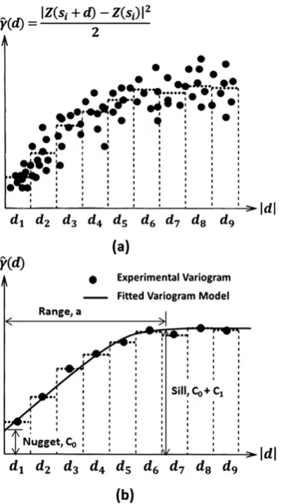
For OK interpolation of variables, first an experimental variogram
b
γð Þd is derived by
b
γð Þ ¼d 1
2N dð Þ ∑ N dð Þ
i¼1
Z sðiþdÞ−Z sð Þi
½ 2 (3)
whereZ(si) andZ(si+d) are the variable values at corresponding
sam-pling locationssiand (si+d), respectively, located atddistance apart
andN(d) is the number of data pairs. A variogram cloud is initially
gen-erated using Equation 3 for observations at any two data points, in
which all semivariance values are plotted against their separation
dis-tance. The experimental variogram is computed from the variogram
cloud by subdividing it into a number of lags and taking an average
of each lag interval (Johnston, VerHoef, Krivoruchko, & Lucas, 2001;
Robertson, 2008). A variogram modelγ(d) is then fitted to the
experi-mental variogram. A typical variogram cloud based on Equation 3 and
a typical experimental variogram with a typical fitted model is shown in
Figure 3.
Exponential, Gaussian, and spherical are the most commonly used
variogram models for kriging applications in hydrology (Adhikary et al.,
2015), which are also used to model the experimental variogram. The
functional forms these variogram models are given in Table 2. The
three models are fitted to the experimental variogram using regression
by noting the residual sum of squares (RSS) between the experimental
b
γð Þdk and modelledγ(dk) variogram values (Mair & Fares, 2011) with a trial‐and‐error approach for different lag sizes and lag intervals
(Goovaerts, 1997) such that the RSS is minimum. RSS is given by
RSS¼ ∑
K
k¼1bγ
dk
ð Þ−γð Þdk
½ 2
(4)
RSS in Equation 4 provides an exact measure of how well the
variogram model fits the experimental variogram (Robertson, 2008).
Lag sizes and number of lags are varied based on a general rule of
thumb, in which the lag size times the number of lags should be about
half of the largest distance among all data pairs in the variogram cloud
(Johnston et al., 2001, p. 66). The variogram parameters (nugget, sill,
and range) are also iteratively changed to obtain the best fitted model.
The model with its corresponding parameters that minimizes RSS is
selected as the best variogram model and finally used in OK analysis.
Variogram model fitting is performed using GS+ geostatistical software
(Robertson, 2008) and OK is implemented through ArcGISv9.3.1
soft-ware (ESRI, 2009) and its geostatistical analyst extension (Johnston
et al., 2001).
3.2
|Ordinary cokriging
OCK method is a modification of the OK method. The key advantage of
OCK is that it can make use of more than one variable rather than using
only a single variable in the estimation process. The OCK method is
used to enhance the estimation of primary variable by using secondary
variable assuming that the variables are correlated to each other (Isaaks
& Srivastava, 1989). In this study, rainfall and elevation are considered,
respectively, as the primary and secondary variables in the OCK
method. Like OK method, the aim of the OCK method is to estimate
the primary variable. The OCK estimator (Goovaerts, 1997) considering
one secondary variable (i.e., elevation), which is cross‐correlated with
the primary variable (i.e., rainfall) may be written as
b
ZOCKð Þ ¼s0 ∑
n
i1¼1 ωOCK
i1 Z sð Þ þi1 ∑ m
i2¼1 ωOCK
i2 V si2
with ∑n i1¼1
ωOCK i1 ¼1; ∑
m
i2¼1 ωOCK
i2 ¼0
(5)
where bZOCKð Þs0 is the estimated value of primary variable at target
unsampled locations0,ωOCKi1 andω OCK
i2 are the kriging weights associated
with the sampling locations of the primary and secondary variablesZ
FIGURE 3 (a) a typical variogram cloud for a finite set of discrete lags, and (b) a typical experimental variogram based on the variogram cloud fitted by a typical variogram model with its parameters
TABLE 2 Commonly used positive‐definite variogram models
Model name Model equation
Exponential γð Þ ¼d C0þC11−exp−3ad
Gaussian γð Þ ¼d C
0þC1 1−exp −3d 2 a2
h i
Spherical γð Þ ¼d C
0þC1 32 d a−
1 2
d3 a3
h i
; d<a
=C0+C1, d≥a
C0= nugget coefficient,C0+C1= Sill,a= range of variogram model.
andV, respectively,nandmare the number of sampling points for the
primary and secondary variables.
The OCK weights are obtained by solving a system of (n+ 2)
simul-taneous linear equations (Goovaerts, 1997) that can be given by
∑n i1¼1γ
zzsi1−sj1
ωOCK i1 þ ∑
m
i2¼1 γzv si2−sj1
ωOCK i2 þμ
OCK
1 ¼γzzsj1−s0
for j1¼1;……;n ∑n
i1¼1γ vzsi1−sj2
ωOCK i1 þ ∑
m
i2¼1γ vvsi2−sj2
ωOCK i2 þμ
OCK
2 ¼γvzsj2−s0
for j2¼1;……;m ∑n
i1¼1ω OCK i1 ¼1
∑ m
i2¼1 ωOCK
i2 ¼0
(6)
where γzv si2−sj1
and γvz si1−sj2
are the cross‐variogram values
between sampled Z and V values, andμOCK
1 andμOCK2 are the Lagrange
multiplier parameters accounting for the two unbiased conditions.
The elementary step in the OCK method is to establish an
appro-priate model for cross continuity and dependency between the
pri-mary (rainfall) and secondary (elevation) variable. This positive
correlation between variables is referred to as the cross‐regionalization
or coregionalization (Goovaerts, 1997; Wackernagel, 2003), which can
be quantified by cross‐variogram or cross‐covariance. These models
are used to define the cross continuity and dependency between
two variables in the OCK method (Subyani & Al‐Dakheel, 2009). The
cross‐variogram models between the primary (rainfall) and secondary
(elevation) variables in the OCK method are obtained by fitting with
an experimental cross‐variogram that is given by
b
γzv¼bγvz¼ 1 2N dð Þ ∑
N dð Þ
i¼1
Z sðiþdÞ−Z sð Þi
½ ×½V sðiþdÞ−V sð Þi (7)
It is important to note that the variogram models must satisfy the
positive‐definite condition (PDC) in kriging. For a single variable
(rain-fall) in the OK method, the condition is satisfied by using the
posi-tive‐definite variogram model functions given in Table 2. However,
the OCK method considering two variables (rainfall and elevation)
con-sists of one cross‐variogram and two direct variograms, and additional
requirement for satisfying the PDC (Goovaerts, 1999). In order to
make sure that the cross‐variogram model is positive‐definite (all
eigenvalues are positive), an indicator called the Cauchy‐Schwarz
inequality (Journel & Huijbregts, 1978; Phillips et al., 1992) must be
satisfied for all distance valuesd, which is given by
γzvð Þd≤½γzzð Þdγvvð Þd 1
2 (8)
whereγzv(d) is the cross‐variogram model between primary and
sec-ondary variables, andγzz(d) andγvv(d) are the direct variogram models
for primary and secondary variables, respectively. Based on the
indica-tor shown in Equation 8, Hevesi et al. (1992) suggested a graphical test
of PDC for the fitted models as follows:
PDC¼½γzzð Þdγvvð Þd 1
2 (9)
The model is considered positive‐definite if the absolute value of
the cross‐variogram modelγzv(d) in Equation 8 is less than the slope
and corresponding absolute value of PDC curve in Equation 9 for all
distance values d. In the OCK method, direct and cross‐variogram
models are fitted as linear combination of the same set of basic models
given in Table 2 such that the RSS value by Equation 4 is minimum
under the requirement of PDC. Variogram model fitting is performed
using GS+ geostatistical software (Robertson, 2008) and OCK is
imple-mented through ArcGISv9.3.1 software (ESRI, 2009) and its
geostatistical analyst extension (Johnston et al., 2001).
3.3
|Kriging with an external drift
KED is a particular type of universal kriging that gives the estimation of
a primary variable Z, known only at a small number of locations in the
study catchment, through a secondary variable V, exhaustively known
in the same area (Feki et al., 2012). The trend or local mean of the
pri-mary variable is first derived using the secondary variable (Goovaerts,
1997; Wackernagel, 2003) and then simple kriging is carried out on
residuals from the local mean. The KED estimator (Wackernagel,
2003) is generally given as
b
ZKEDð Þ ¼s0 ∑
n
i¼1ω
KED
i Z sð Þi with ∑ n
i¼1ω
KED
i ¼1 (10)
The KED weights ωKED
i can be obtained by solving a system of
(n+ 2) simultaneous linear equations as follows:
∑n i¼1γR
si−sj
ωKED
i þμKED0 þμKED1 V sj ¼γR sj−s0
for j¼1;… …;n
∑n i¼1ω
KED i ¼1
∑n i¼1ω
KED
i V sð Þ ¼i V sð Þ0
;
(11)
where γR(si−sj) is the residual variogram values between sampling
locationssiandsj,γR(sj−s0) is the residual variogram values between
sampling locationsjand the target location,s0, andμKED0 andμKED1 are
the Lagrange multiplier parameters.
OCK and KED differ in the way the secondary variableVis used.
The secondary variable (e.g., elevation in this study) gives only the
trend information in KED, whereas estimation with OCK is directly
influenced by it (Delbari et al., 2013). In case of KED, the primary
and secondary variables should exhibit a linear relationship. In addition,
estimation with KED requires the secondary variable values at all the
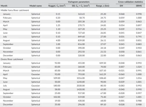
TABLE 3 Results of fitted variogram models for monthly rainfall data for using in the OK interpolation method
Month Model name
Variogram parameters Cross‐validation statistics Nugget, C0(mm2) Sill, C0+ C1(mm2) Range, a (km) SM SRMS
Middle Yarra River catchment
January Spherical 0.15 163.65 25.20 0.068 0.998
February Spherical 0.20 58.70 24.75 0.059 1.000
March Spherical 0.00 205.38 25.25 0.059 0.863
April Spherical 1.25 270.75 24.85 0.054 0.897
May Spherical 1.10 327.20 25.25 0.039 0.916
June Spherical 0.10 727.60 26.85 0.041 0.847
July Spherical 0.10 849.60 27.00 0.031 0.795
August Spherical 4.00 839.00 26.11 0.035 0.851
September Spherical 1.00 816.00 27.07 0.045 0.883
October Spherical 0.00 390.00 24.18 0.049 0.903
November Spherical 0.00 292.50 21.53 0.058 0.861
December Spherical 0.00 320.00 22.00 0.060 0.863
Ovens River catchment
January Spherical 92.00 455.00 109.50 ‐0.048 0.992
February Spherical 83.00 360.00 70.00 0.007 1.024
March Spherical 85.00 501.00 107.10 ‐0.021 0.991
April Gaussian 93.00 793.00 162.29 ‐0.060 1.000
May Spherical 109.00 1016.00 108.60 ‐0.047 1.016
June Spherical 50.00 1240.00 90.00 ‐0.039 1.001
July Gaussian 180.00 2030.00 80.50 ‐0.083 0.992
August Spherical 58.00 1420.00 65.00 ‐0.040 0.990
September Spherical 25.00 937.00 67.00 ‐0.028 0.997
October Spherical 102.00 519.00 75.40 ‐0.027 1.001
November Spherical 19.00 430.00 68.00 0.001 0.988
December Spherical 35.00 296.00 89.10 ‐0.028 0.988
estimation grid nodes as well as all the sampling locationssi. The
resid-ual variogram models are fitted based on the basic models in Table 2
such that the RSS value between the experimental and modelled
variogram values by Equation 4 is minimum. Variogram model fitting
and estimation with KED are performed using GS+ geostatistical
soft-ware (Robertson, 2008).
3.4
|Inverse distance weighting
IDW interpolation method (ASCE, 1996) gives a linear weighted
aver-age of several neighbouring observations to estimate the variable value
at target location. This method assumes that each observation point
has local influence that diminishes with distance. IDW assigns greater
weights to observation points near to the target location, and the
weights diminish as a function of distance (Johnston et al., 2001).
The estimation by IDW can be written as
b
Z sð Þ ¼0 ∑
n
i¼1ωi
Z sð Þi where ωi¼d−i0k=∑
n
i¼1
d−i0k (12)
wherebZ sð Þ0 is the estimated rainfall value at desired locations0,Z(si) is
the Z value at location si,ωiis the weight assigned to observation
points,di0is the distance between the sampling point at locationssi
ands0,nis the number of sampling points, andkis a power, which is
referred to as a control parameter.
As“k” approaches zero and the weights becomes more similar,
IDW estimates approach the simple average of the surrounding
obser-vations. However, the effect of the farthest observations on the
estimated value is diminished with the increase ofk. The value ofk
ranges from 1 to 6 (Teegavarapu & Chandramouli, 2005). Several
stud-ies have investigated with variations in a power to examine its effects
on the spatial distribution of information from rainfall observations
(Chen & Liu, 2012). Therefore,kvalue is varied in the range of 1 to 6
with an increment of 0.1 in the current study. The optimalkvalue is
selected based on the lowest RMSE value between the observed and
estimated values. All rain‐gauge stations are considered in the search
neighbourhood in the estimation process. IDW interpolation is
per-formed by ArcGISv9.3.1 software (ESRI, 2009) and its geostatistical
analyst extension (Johnston et al., 2001).
3.5
|Radial basis function
RBF (Chilès & Delfiner, 1999) is an exact interpolation method, which
stands for a diverse group of interpolation methods. The RBF
estima-tor can be viewed as a weighted linear function of distance from grid
point to data point plus a bias factor, which is given by
b
Z sð Þ ¼0 ∑
n
i¼1ωi∅
si−s0
k k
ð Þ þμ (13)
where∅(r) is the radial basis function (r=‖si−s0‖),ris the radial
dis-tance from target point s0to sampling pointssi,ωiare the weights
andμis the Lagrangian multiplier. The weights are obtained by solving
of a system of (n+ 1) simultaneous linear equations.
The basis kernel functions in the RBF method are analogous to
variograms in kriging, which makes it similar to geostatistical
interpola-tion methods. However, RBF does not have the advantage of a prior
analysis of spatial correlation unlike kriging. When interpolating a grid
node, the basis kernel functions define the optimal set of weights to be
used with the sampling points. There are several radial basis functions
available (Johnston et al., 2001) However, thin plate spline is the most
commonly used radial basis function for interpolation (e.g., Boer, de
Beurs, & Hartkamp, 2001; Di Piazza et al., 2011; Hutchinson, 1995).
In this study, thin plate spline is also used as the radial basis function,
which is given by
∅ð Þ ¼r ð Þcr2lnð Þcr (14)
wherecis the smoothing parameter, which is obtained through cross‐
validation process. The optimal value of the smoothing parameter is
selected based on the lowest RMSE value between the observed and
estimated values. RBF interpolation method is performed by
ArcGISv9.3.1 software (ESRI, 2009) and its geostatistical analyst
extension (Johnston et al., 2001).
3.6
|Assessment of interpolation methods
The performance of different interpolation methods (OK, OCK, KED,
IDW, and RBF) used in this study are evaluated and compared through
cross‐validation process. The cross‐validation is a simple leave‐one‐out
validation procedure (Haddad, Rahman, Zaman, & Shrestha, 2013) in
which observations are removed one at a time from the dataset and
then re‐estimated from the remaining observations using the adopted
model. Cross‐validation provides important evidence of the
perfor-mance measures for the interpolation methods. In this study, the
per-formance of all the interpolation methods for rainfall estimation is
compared based on mean bias error (MBE), RMSE, and coefficient of
determination (R2) values between the observed and estimated rainfall
values, which are given by Equations 15–17.
MBE¼1
n∑ n
i¼1
Z sð Þi−bZ sð Þi
h i
(15)
RMSE¼
ffiffiffiffiffiffiffiffiffiffiffiffiffiffiffiffiffiffiffiffiffiffiffiffiffiffiffiffiffiffiffiffiffiffiffiffiffiffiffi
1
n∑ n
i¼1
Z sð Þi−bZ sð Þi
h i2
s
(16)
R2¼ ∑
n
i¼1fZ sð Þi−Zmg bZ sð Þi −bZm
n o
h i2
∑n
i¼1fZ sð Þi−Zmg2∑ni¼1 bZ sð Þi −Zbm
n o2 (17)
In Equations 15–17,Z(si) andbZ sð Þi are the observed and predicted
values,ZmandbZmare the mean of the observed and predicted values, andnis the number of sampled data points. The interpolation method
with the lowest MBE and RMSE values and the highestR2value is
cho-sen as the best interpolation method.
As has been mentioned earlier, kriging gives the prediction
standard error while giving the estimation of unsampled variables,
the adequacy of the variogram model for kriging and cokriging
estima-tion should also be tested to produce correct interpolaestima-tion results
(Johnston et al., 2001; Phillips et al., 1992). Therefore, two additional
standardized cross‐validation statistics are used in this study, which
are standardized mean error (SM) and standardized root mean square
error (SRMS) as given by Equations 18–19
SM¼1
n∑ n
i¼1
Z sð Þi −Z sbð Þi
h i
b
σð Þsi
(18)
SRMS¼
ffiffiffiffiffiffiffiffiffiffiffiffiffiffiffiffiffiffiffiffiffiffiffiffiffiffiffiffiffiffiffiffiffiffiffiffiffiffiffiffi
1
n∑ n
i¼1
Z sð Þi−bZ sð Þi
b
σð Þsi
" #2
v u u
t (19)
wherebσð Þsi is the prediction standard error for locationsi. SM should be close to 0 if the estimates using the adopted variogram model are
unbiased. SRMS should be close to 1 if the estimation variances are
consistent and the variability of the prediction is correctly assessed
(Adhikary et al., 2015; Johnston et al., 2001).
4
|R E S U L T S A N D D I S C U S S I O N
4.1
|Variogram models for OK analysis
The OK analysis requires the estimation of the direct variogram models
for rainfall data. In this study, an isotropic experimental variogram is
estimated from the rainfall dataset for each month assuming an
identi-cal spatial correlation in all directions and neglecting the influence of
anisotropy on the variogram parameters. Isotropy is assumed for the
methodological simplicity. Isotropy is a property of a natural process
or data where directional influence is considered insignificant and
spa-tial dependence (autocorrelation) changes only with the distance
between two locations (Johnston et al., 2001). Under the isotropic
con-dition, the semivariance is assumed the same for a given distance,
regardless of direction. Initially, the directional experimental variograms
are estimated from each monthly rainfall dataset. However, the
direc-tional variograms are found noisy because of the less number of rain‐
gauge stations in the study area. Therefore, the directional influence
is ignored in the experimental variogram calculation. The experimental
variogram is then fitted with three predefined variogram model
func-tions (exponential, Gaussian, and spherical as given in Table 2) to obtain
the variogram models for each monthly rainfall dataset.
For convenience in this study, results obtained for the Middle
Yarra River catchment are presented and discussed elaborately and
compared with that obtained for the Ovens River catchment.
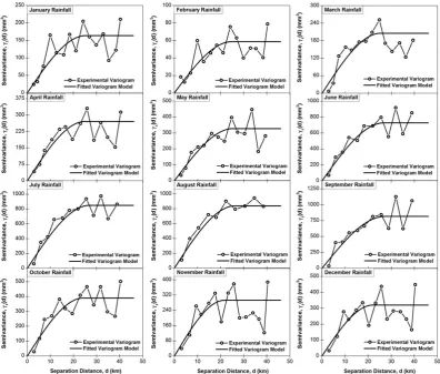
Figure 4 shows the experimental variograms and fitted variogram
models with optimal variogram parameters (i.e., nugget, sill, and range)
for monthly rainfall data of the Middle Yarra River catchment, which
are used in OK analysis. The best fitted variogram models are selected
based on the minimum RSS values using a trial‐and‐error process with
different lag intervals. The variogram parameters are iteratively
changed to get the best fitted model, which yields the minimum RSS.
As can be seen from Figure 4, the spherical model is the best fitted
variogram model for all months having spatial structure of
.66 <R< .97 (results ofRnot shown in Figure). It can be also noted that
10 months (except November and December) haveRvalues greater
than .75. The optimal variogram parameters for each monthly rainfall
dataset for both the catchments are provided in Table 3. As can be
seen from Table 3, the ratio of nugget coefficient to sill of the
variogram model is small for all months for both the catchments. This
evidently indicates that a strong spatial correlation exists between
the monthly mean rainfall and the spatial distribution of the rain‐gauge
stations over the study area. This supports the use of geostatistical
interpolation methods such as OK, OCK, and KED, which consider
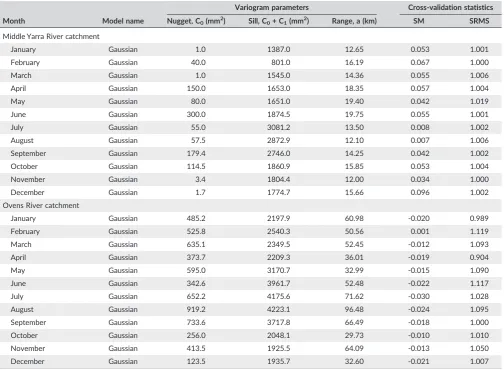
TABLE 4 Results of fitted cross‐variogram models between monthly rainfall and elevation for using in the OCK interpolation method
Month Model name
Variogram parameters Cross‐validation statistics Nugget, C0(mm2) Sill, C0+ C1(mm2) Range, a (km) SM SRMS
Middle Yarra River catchment
January Gaussian 1.0 1387.0 12.65 0.053 1.001
February Gaussian 40.0 801.0 16.19 0.067 1.000
March Gaussian 1.0 1545.0 14.36 0.055 1.006
April Gaussian 150.0 1653.0 18.35 0.057 1.004
May Gaussian 80.0 1651.0 19.40 0.042 1.019
June Gaussian 300.0 1874.5 19.75 0.055 1.001
July Gaussian 55.0 3081.2 13.50 0.008 1.002
August Gaussian 57.5 2872.9 12.10 0.007 1.006
September Gaussian 179.4 2746.0 14.25 0.042 1.002
October Gaussian 114.5 1860.9 15.85 0.053 1.004
November Gaussian 3.4 1804.4 12.00 0.034 1.000
December Gaussian 1.7 1774.7 15.66 0.096 1.002
Ovens River catchment
January Gaussian 485.2 2197.9 60.98 ‐0.020 0.989
February Gaussian 525.8 2540.3 50.56 0.001 1.119
March Gaussian 635.1 2349.5 52.45 ‐0.012 1.093
April Gaussian 373.7 2209.3 36.01 ‐0.019 0.904
May Gaussian 595.0 3170.7 32.99 ‐0.015 1.090
June Gaussian 342.6 3961.7 52.48 ‐0.022 1.117
July Gaussian 652.2 4175.6 71.62 ‐0.030 1.028
August Gaussian 919.2 4223.1 96.48 ‐0.024 1.095
September Gaussian 733.6 3717.8 66.49 ‐0.018 1.000
October Gaussian 256.0 2048.1 29.73 ‐0.010 1.010
November Gaussian 413.5 1925.5 64.09 ‐0.013 1.050
December Gaussian 123.5 1935.7 32.60 ‐0.021 1.007
the spatial correlation in the estimation process. The range of influence
and the sill of the variogram model vary from one month to another,
but the variogram exhibit a same spherical structure in all months. This
may be caused due to the control of the relief on the spatial
distribu-tion of rainfall (Delbari et al., 2013). The range of influence is lowest
for November (21.53 km) and highest for September (27.07 km).
Fur-thermore, the cross‐validation statistics in Table 3 for both the
catch-ments confirm that the fitted variogram models for all monthly
rainfall data satisfy the unbiased condition and thus can be used for
the OK analysis.
For elevation data, an isotropic experimental variogram is
com-puted ignoring the directional influence. The experimental variogram
is then fitted with the aforementioned three variogram model
func-tions. The best fitted variogram model is selected using the same
pro-cedure described above. The Gaussian variogram model gives the best
fitted model for both the catchments with the lowest RSS value, which
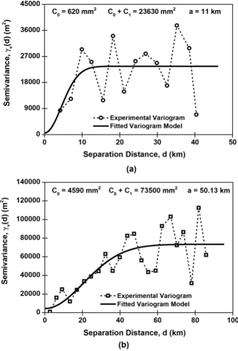
is shown in Figure 5. The optimal variogram parameters for both the
catchments are also shown in the figure. In order to avoid possible
inconsistencies in the subsequent modelling of direct and cross‐
variograms in OCK analysis (Goovaerts, 1997, 2000), the colocated
elevation data (see Figure 1) are used for estimating the variogram of
elevation, not the entire DEM of the catchment. Therefore, the
cokriging method adopted in this study is referred to as the colocated
OCK method (Wackernagel, 2003).
4.2
|Cross
‐
variogram models for OCK analysis
The OCK analysis requires the simultaneous estimation of the direct
and cross‐variogram models for the rainfall and elevation variables.
The three variogram models are fitted as a linear combination of the
same set of standard models given in Table 2 so that the RSS value is
minimum under the constraints of PDC (Goovaerts, 1999). Figure 6
shows the experimental and fitted cross‐variogram models for the
Middle Yarra River catchment. The number of data pairs in each lag size
is the same for all the three direct and cross‐variogram models.
Figure 6 also shows the PDC curve computed based on Equation 9
to examine the positive‐definiteness criteria of the cross‐variogram
models obtained for the catchment. Additionally, the cross‐validation
statistics are used for identifying the adequacy and final selection of
the adopted cross‐variogram model for the OCK analysis. The cross‐
validation results obtained using all the adopted cross‐variogram
models for both the catchments are presented in Table 4. The results in
Table 4 indicate that the cross‐variogram models of all monthly
datasets are suitable for the OCK analysis considering all
neighbourhoods for both the catchments.
As can be seen from Figure 6, the Gaussian variogram model fits
well for all monthly datasets of the Middle Yarra River catchment,
which also satisfy the PDC criteria defined by Equation 9.
Further-more, the correlation between monthly rainfall and elevation for all
months in Table 1 indicates that elevation will contribute to enhance
the monthly rainfall estimation in the catchment. The figure also shows
that the values of the sample cross‐variogram increase for distances
from 0 to 25 km (more than half of the maximum interstation distance)
for almost all months. This indicates that a positive spatial cross‐
correlation exists between rainfall and elevation in the catchment. This
wide ranges may be due to the high correlation (.67 <R< .79) between
the monthly rainfall and elevation (Table 1). Such high correlation
con-firms that the monthly rainfall in the Middle Yarra River catchment is
mainly caused by the orographic effects.
Figure 6 also shows the PDC curves, which are computed to
examine the positive‐definite conditions of the cross‐variogram
models of the catchment. It is worth pointing out that the PDC curve
may give a qualitative indication for the degree of correlation. As can
be observed from Figure 6, the plotted PDC curve for most of the
months showed a close fit to the cross‐variogram model for smaller
distances with few exceptions (February, April, May, and June
months). For example, the PDC curve is closer to the cross‐variogram
model in the case of January, March, July, November, and December
months depending on the degree of correlation. This conclusion holds
true based on the higher correlation for these months as given in
Table 1.
4.3
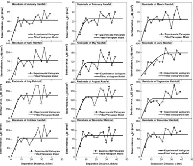
|Residual variogram models for KED analysis
In order to implement the KED analysis, experimental residual
variograms are estimated based on the residuals obtained from linear
regression between rainfall and elevation data neglecting the influence
of anisotropy on the variogram parameters. The experimental residual
variogram is then fitted using the three standard models given in
Table 2. Figure 7 shows the experimental and fitted residual variogram
models for all monthly datasets of the Middle Yarra River catchment. It
can be seen from the figure that the spherical model gives the best
fitted model for all monthly datasets. The optimal variogram
parame-ters and the corresponding cross‐validation statistics of the selected
residual variogram models for both the catchments are presented in
Table 5. As can be also seen from Figure 7 and Table 5, the residual
variogram models exhibit relatively smaller sills than those obtained
from the actual rainfall datasets (see Figure 4) but they follow very
sim-ilar structure. This is not unexpected because the residual variograms
from the linear regression represents variation, which remains after
removing the trend (Lloyd, 2005). The cross‐validation statistics shown
in Table 5 also indicate that the residual variogram models of all
monthly datasets for both the catchments are satisfactory for the
KED analysis.
TABLE 5 Results of fitted residual variogram models for using in the KED interpolation method
Month Model name
Variogram parameters Cross‐validation statistics Nugget, C0(mm2) Sill, C0+ C1(mm2) Range, a (km) SM SRMS
Middle Yarra River catchment
January Spherical 0.10 43.14 8.86 0.029 1.022
February Spherical 0.01 23.11 13.10 0.025 0.981
March Spherical 0.10 56.69 9.35 0.060 0.999
April Spherical 0.10 75.70 10.76 0.010 1.000
May Spherical 0.10 115.80 11.61 ‐0.034 1.031
June Spherical 39.90 298.70 27.03 0.005 0.981
July Spherical 5.70 257.70 11.59 ‐0.024 0.990
August Spherical 0.10 265.00 11.57 ‐0.013 0.984
September Spherical 0.10 283.50 11.77 0.027 0.982
October Spherical 0.10 139.40 10.60 ‐0.010 1.004
November Spherical 0.10 84.94 9.69 0.054 0.992
December Spherical 0.10 100.70 10.61 0.058 0.990
Ovens River catchment
January Spherical 38.90 239.40 42.90 ‐0.017 1.012
February Spherical 60.10 320.90 32.72 0.004 1.029
March Spherical 13.40 246.20 26.80 ‐0.011 0.996
April Gaussian 67.20 188.00 103.05 ‐0.043 1.008
May Spherical 217.00 597.00 108.40 ‐0.026 1.071
June Spherical 60.00 841.00 70.20 ‐0.044 1.028
July Spherical 5.00 1713.00 106.00 ‐0.092 1.005
August Gaussian 250.00 2084.00 90.54 ‐0.045 1.001
September Spherical 1.00 975.00 100.85 ‐0.027 1.029
October Spherical 42.10 383.60 87.00 ‐0.018 1.041
November Spherical 6.00 367.30 92.30 ‐0.012 0.989
December Spherical 31.00 192.50 88.75 ‐0.028 0.993
4.4
|Spatial prediction of rainfall
In this study, different geostatistical and deterministic interpolation
methods including OK, OCK, KED, IDW, and RBF are adopted to
estimate the spatial distribution of monthly mean rainfall in the
Middle Yarra River catchment and the Ovens River catchment in
Australia. Several performance measures including MBE, RMSE, and
R2 are frequently used to indicate how accurately an interpolator
predicts the observed data. Smaller values of MBE and RMSE with
a higher R2 value of an interpolator indicate better prediction by
the corresponding method. In case of the scatter plot, the better
pre-diction is that if all scattered points lay close to the 450line with the
highest R2 value between the predicted and observed values
(Adhikary et al., 2016a).
Table 6 presents the different performance measures of the
adopted interpolation methods (or interpolators) for estimating
monthly rainfall over both the study catchments. The different
interpo-lation methods are quantitatively compared based on these
perfor-mance measures in order to identify the best interpolator for each of
the catchment. As can be seen from the table, geostatistical (OK,
OCK, and KED) interpolation methods perform better than
determinis-tic (IDW and RBF) interpolation methods for monthly rainfall
estima-tion in the study area. The OCK method gives the best results for
rainfall estimation over the study area for all months when considering
all the performance measures. The KED method gives the second best
results, which is very close to the performance of the OCK method but
performs better than the OK method for both the catchments. IDW
and RBF give similar performance with higher error in rainfall
estima-tion over the study area. For the Middle Yarra River catchment,
Table 6 also shows that in some months, the RBF method performs
better than the OK method for rainfall estimation. However, no
remarkable differences are seen between them when considering all
the performance measures.
For OK, OCK, KED, IDW, and RBF methods, the average RMSE
values (Table 6) for the Middle Yarra River catchment are 11.93,
10.29, 10.85, 12.66, and 12.22 mm, respectively, whereas the average
RMSE values for the Ovens River catchment are 17.42, 16.15, 16.65,
17.54, and 23.41 mm, respectively. For OK, OCK, KED, IDW, and
TABLE 6 Performance of different interpolation (OK, OCK, KED, IDW, and RBF) methods for monthly rainfall estimation in the study area
Month
MBE (mm) RMSE (mm) R2
OK OCK KED IDW RBF OK OCK KED IDW RBF OK OCK KED IDW RBF
Middle Yarra River catchment
January 0.98 0.63 0.73 1.76 1.56 8.92 6.96 7.99 8.96 9.99 0.40 0.66 0.56 0.42 0.31
February 0.51 0.38 0.41 0.73 0.85 5.25 3.80 4.45 5.26 5.46 0.42 0.71 0.59 0.42 0.42
March 0.97 0.65 0.70 1.67 1.78 8.71 6.79 8.41 9.58 9.50 0.54 0.73 0.58 0.45 0.46
April 1.03 0.83 0.89 1.70 2.27 9.80 8.26 8.75 10.68 10.04 0.54 0.67 0.64 0.46 0.55
May 0.78 0.72 ‐0.40 1.43 2.41 11.55 10.78 11.98 11.58 11.80 0.49 0.56 0.51 0.49 0.55
June 1.19 1.26 1.17 2.25 3.29 15.15 13.77 13.44 17.26 15.15 0.61 0.67 0.69 0.49 0.63
July 0.89 0.11 ‐0.36 1.73 2.77 15.50 14.63 14.84 16.85 15.01 0.65 0.69 0.68 0.59 0.68
August 1.05 0.03 ‐0.20 2.08 3.04 16.75 15.94 14.67 18.19 16.12 0.59 0.63 0.69 0.52 0.64
September 1.38 0.87 0.92 2.69 3.52 16.79 15.73 15.38 18.46 17.17 0.57 0.62 0.63 0.48 0.57
October 1.07 0.79 ‐0.11 1.86 2.32 12.34 10.70 11.56 12.05 12.48 0.53 0.64 0.60 0.56 0.56
November 1.23 0.55 0.58 2.16 2.28 11.00 8.25 9.10 11.43 11.72 0.50 0.73 0.66 0.47 0.46
December 1.31 1.07 1.08 2.25 2.28 11.43 7.93 9.58 11.65 12.17 0.51 0.78 0.66 0.50 0.48
Average 1.03 0.66 0.45 1.86 2.36 11.93 10.29 10.85 12.66 12.22 0.53 0.67 0.62 0.49 0.54
Ovens River catchment
January ‐0.62 ‐0.56 ‐0.25 ‐1.78 ‐1.13 12.86 12.39 12.45 13.68 18.42 0.41 0.44 0.42 0.34 0.18
February 0.11 ‐0.01 0.08 ‐0.96 1.26 17.51 16.32 17.34 17.53 25.64 0.15 0.23 0.19 0.11 0.02
March ‐0.28 ‐0.22 ‐0.15 ‐1.26 ‐0.25 13.13 12.30 12.87 14.44 17.14 0.44 0.59 0.51 0.33 0.32
April ‐0.62 ‐0.38 ‐0.41 ‐0.53 ‐0.58 10.31 9.19 9.58 11.00 14.91 0.56 0.71 0.66 0.49 0.31
May ‐1.07 ‐0.59 ‐0.60 ‐1.94 ‐1.56 23.18 21.16 22.89 23.27 34.19 0.18 0.29 0.25 0.15 0.01
June ‐0.92 ‐0.87 ‐0.94 ‐1.19 ‐0.81 22.13 21.98 22.04 22.21 32.50 0.52 0.66 0.61 0.57 0.30
July ‐1.94 ‐1.36 ‐2.01 ‐3.53 ‐2.09 23.16 22.89 22.92 23.01 31.35 0.62 0.68 0.65 0.64 0.44
August ‐0.94 ‐0.92 ‐1.05 ‐1.35 ‐1.16 22.24 21.92 21.97 22.27 30.01 0.66 0.70 0.68 0.68 0.49
September ‐0.62 ‐0.55 ‐0.62 ‐0.46 ‐0.87 20.39 20.01 20.08 20.44 28.12 0.50 0.57 0.54 0.56 0.32
October ‐0.53 ‐0.31 ‐0.35 ‐0.63 ‐0.41 19.37 17.65 19.01 19.64 26.24 0.23 0.39 0.32 0.19 0.04
November 0.01 ‐0.33 ‐0.05 0.18 0.30 10.52 9.37 9.48 12.17 11.61 0.73 0.80 0.78 0.65 0.70
December ‐0.27 ‐0.21 ‐0.11 ‐0.41 ‐0.22 9.67 8.59 9.12 10.82 10.83 0.63 0.71 0.69 0.54 0.61
Average ‐0.64 ‐0.53 ‐0.54 ‐1.15 ‐0.63 17.42 16.15 16.65 17.54 23.41 0.47 0.57 0.53 0.44 0.31
Note. IDW = inverse distance weighting; KED = kriging with an external drift; MBE = mean bias error; OCK = ordinary cokriging; OK = ordinary kriging;