Jacobian
Robert Dry lo
Institute of Mathematics, Polish Academy of Sciences, Warsaw School of Economics, Poland
Abstract. Genus 2 curves with simple but not absolutely simple jacobians can be used to construct pairing-based cryptosystems more efficient than for a generic genus 2 curve. We show that there is a full analogy between methods for constructing ordinary pairing-friendly elliptic curves and simple abelian varieties, which are iogenous over some extension to a prod-uct of elliptic curves. We extend the notion of complete, complete with variable discriminant, and sparse families introduced in by Freeman, Scott and Teske [11] for elliptic curves, and we generalize the Cocks-Pinch method and the Brezing-Weng method to construct families of each type. To realize abelian surfaces as jacobians we use of genus 2 curves of the form
y2=x5+ax3+bxory2=x6+ax3+b, and apply the method of Freeman and Satoh [10].
As applications we find some families of abelian surfaces with recordedρ-valueρ= 2 for em-bedding degreesk= 3,4,6,12, orρ= 2.1 fork= 27,54. We also give variable-discriminant families with bestρ-values.
Keywords: Pairing-friendly hyperelliptic curves, abelian varieties, Weil numbers, CM method.
1 Introduction
Since pairings have been introduced to design cryptographic protocols (see, e.g., [2, 3, 20, 35]), one of the main problems is to construct abelian varieties suitable for these applica-tions. Let A/Fq be an abelian variety containing an Fq-rational subgroup of prime order
r with the embedding degree k= min{l:r |(ql−1)}. To implement pairing-based cryp-tosystemskshould be suitably small so that pairings ofr-torsion points with values in the fieldFqk could be efficiently computed, but the discrete logarithm problem inFqk remains intractable. Furthermore, in order the arithmetic onAto be more efficient, we would like that the bit size ofr to be close to the size of #A(Fq). Since log(#A(Fq))≈dimAlog(q),
we would like the parameterρ= dimAlogq/logrto be close to one. We can achieveρ≈1 using supersigular abelian varieties, which in each dimension have bounded embedding degrees (e.g., k≤6 or 12 for supersingular elliptic curves or abelian surfaces (see [14, 29, 31])). For higher security levels we use ordinary varieties, which are unlikely to be found by a random choice and require specific constructions. In practice, we mainly use elliptic curves or jacobians of hyperelliptic curves of low genus.
Pairing-friendly elliptic curves.In general, to construct an ordinary elliptic curve E with an embedding degree kwe first find parameters (r, t, q) of E, wheret is the trace of E,q
curves are generated either directly, like in the Cocks-Pinch method (see [11, Theorem 4.1]), or are obtained as values of suitable polynomials (r(x), t(x), q(x)) called parametric families. The former method is very flexible and allows one to obtain the subgroup orders
r and discriminantsdof almost arbitrary size, however with ρ-value only around 2. Using parametric families we can considerably improve ρ-values for more restricted subgroup orders and discriminants.
Miyaji, Nakabayashi and Takano [25] were the first researchers to use parametric fami-lies to characterize elliptic curves of prime orders with embedding degreesk= 3,4,6. Scott and Barreto [32], and Galbraith et al. [15] generalized their idea to describe elliptic curves with prescribed cofactors fork= 3,4,6. Currently constructions of families withρ= 1 are yet known for k = 10 and 12, and were discovered by Freeman [8] and Barreto-Naehrig [1], respectively. Most families used in practice are so-called complete families, and are constructed by the Brezing-Weng method [4]. We now recall the general definition and classification of families introduced by Freeman, Scott and Teske [11].
Definition 1. ([11, Definition 2.7]) Letkanddbe positive integers such thatdis square-free. We say that a triple of polynomials (r(x), t(x), q(x)) inQ[x]parametrizes a family of
elliptic curves with embedding degree k and discriminant dif the following conditions are satisfied:
1. q(x) =p(x)s for somes≥1 and p(x) that represents primes.
2. r(x) is irreducible, non-constant, integer valued, and has positive leading coefficient. 3. r(x) divides q(x) + 1−t(x).
4. r(x) divides Φk(t(x)−1), where Φk(x) is thekth cyclotomic polynomial.
5. The CM equation 4q(x)−t(x)2 =dy2 has infinitely many integer solutions (x, y).
Properties of the CM equation lead us to the classification of families. It is clear that we can write 4q(x)−t(x)2 =f(x)g(x)2, wheref(x)∈Z[x] is square-free andg(x)∈Q[x].
Then condition (5) implies by Siegel’s theorem that degf(x)≤2 (see [8, Proposition 2.10] or Lemma 16). We say that a family iscompleteiff =d; then the CM equation is satisfied for any x ∈ Z. We say that a family is complete with variable discriminant if degf = 1;
then substituting x ← (dx2 −b)/a, where f(x) = ax+b, yields a complete family with discriminant d if conditions (1) and (2) of Definition 1 are satisfied. A family is called
sparse if degf = 2; then the CM equation can be transformed to the generalized Pell equation, whose solutions grow exponentially. We note that the Brezing-Weng method [4] can be generalized to construct families of the latter two types (see [7]). These families can be used to generate elliptic curves with larger discriminant, which may be desired for larger randomness of cryptosystems.
Pairing-friendly genus 2 curves. There is also a great deal of interest in constructing pairing-friendly genus 2 curves. Freeman, Stevenhagen and Streng [12] give a general method to generate pairs (r, π) such that π is a Weil q-number corresponding by the Honda-Tate theory to a simple ordinary abelian variety with embedding degreekwith re-spect tor. In order to realize these varieties as jacobians, we must choseπ from a suitable CM field K, where Weil numbers in question are characterized by the condition
NK/Q(π−1)≡Φk(ππ¯)≡0 (modr).
If [K :Q] = 2g, then the corresponding varieties are of dimension g withρ-value around
vari-eties. In order to obtain pairing-friendly ordinary abelian surfaces, which generically have
ρ-value around 4, or less than 4 for parametric families, we use genus 2 curves, whose jacobian is simple but not absolutely simple. Kawazoe and Takahashi [23] use curves of the form y2 = x5+ax and a closed formula for their order [13] (see also Kachisa [21]). Freeman and Satoh [10] give a general method to construct an elliptic curve, whose Weil restriction over some extension contains an abelian surface with a given embedding degree. To realize that surface as a jacobian, they use curves of the form y2 =x5+ax3+bx or
y2 = x6 +ax3 +b. Recently Guillevic and Vergnaud [17] extended their method using closed formulas for the order of these curves.
Contribution. In this paper we show that there is a full analogy between methods for constructing pairing-friendly elliptic curves and simple abelian varieties which are isoge-nous over some extension to a product of elliptic curves. Now we outline the main idea of our method. Let K be a CM field of degree 2g, and suppose that we have a polyno-mial π(x, y) ∈ K[x, y] such that q(x, y) = π(x, y)¯π(x, y) ∈ Q[x, y] and the image π(Z2)
contains “sufficiently many” Weil numbers in K. Then we can use π(x, y) to generate pairing-friendly Weil numbers analogously as in the Cooks-Pinch method. If r is a prime such that the system
NK/Q(π(x, y)−1) =Φk(q(x, y)) = 0, (1)
has solutions over Fr, then we check whether π(x, y) is a Weil number for lifts x, y ∈ Z
of these solutions. Since generically solutions over Fr are of the similar size as r, the
resulting varieties have ρ-value ρ = glogq(x, y)/logr ≈ 2gdegπ(x, y). Thus to obtain
ρ-value around 2g, we need suitable polynomialsπ(x, y) of degree one. IfK contains an imaginary quadratic subfield K0 =Q(
√
−d), then for any u ∈K such that c= uu¯ ∈ Q, the polynomial π(x, y) =u(x+y√−d) satisfies q(x, y) = π(x, y)¯π(x, y) = c(x2 +dy2) ∈
Q[x, y], however, ifc6= 1, then the imageπ(Z2) does not contain sufficiently many primes.
Therefore we will use π(x, y) =ζs(x+y
√
−d) to generate Weil numbers in the CM field
K = Q(ζs,
√
−d), where ζs is an sth primitive root of unity and d > 0 is a square-free
integer. We note that Weilq-numbers of the formπ=ζsπ0 withπ0∈Q(
√
−d) correspond to simple abelian varieties which are isogenous over Fqs to a power of an elliptic curve
E/Fq with the Weil q-numberπ0 (see Corollary 4).
To generalize the Cocks-Pinch and the Brezing-Weng methods we describe in Section 3 prime finite fields and number fields, where system (1) has solutions forπ(x, y) =ζs(x+
y√−d), and we give explicit formulas on solutions. In Section 4 we focus on constructing genus 2 curves, whose jacobian corresponds to Weil numbersπ=ζsπ0in a quartic CM field
K =Q(ζs,
√
−d). We give an algorithm to construct curves of the formy2 =x6+ax3+band
y2=x5+ax3+bx, which is based on the method of Freeman and Satoh (see [10, Algorithm 5.11]). In Section 5 we generalize on abelian varieties Definition 1 and classification of families of elliptic curves. In Sections 6, 7, 8 we generalize the Brezing-Weng method to construct families of each type.
2 Background
In this section we gather basic facts on abelian varieties, which will be needed in the sequel (for details see [26, 37–40]).
Let A/Fq be a g-dimensional abelian variety with qth Frobenius endomorphism πA,
and its characteristic polynomial fA. Then we have fA(πA) = 0, and #A(Fq) = fA(1).
Furthermore, all roots of fA are Weil q-numbers. Recall that an algebraic integer π is
called a Weil q-number if |α(π)| = √q for every embedding α : Q(π) → C). We say
that A is simple if it is not isogenous over Fq to a product of two positive dimensional
abelian varieties. By the Honda-Tate theorem the map which associates the Frobenius endomorphismπA to a simple abelian variety A/Fq induces a one-to-one correspondence
between isogeny classes of simple abelian varieties over Fq and conjugacy classes of Weil
q-numbers. Recall also that a variety Ais called ordinary if it has the maximum number
pg of allp-torsion points over Fq, wherep= charFq. We have the following.
Theorem 2. ([40]) Let A/Fq be a simple abelian variety of dimension g with the endo-morphism algebra K = EndFq(A)⊗Q. Then A is ordinary if and only if K = Q(πA)
is a CM field of degree 2g, and πA, πA are relatively prime in OK. Furthermore, if A is ordinary, thenfA is the minimal polynomial ofπA, and
#A(Fq) =fA(1) = NK/Q(πA−1). (2)
Recall that a number field K is called a CM field if it is an imaginary quadratic extension of a totally real field. Then K has an automorphism, denoted by a bar, which commutes with every embeddingK →Cand the complex conjugation in C.
In this paper we are interested in simple abelian varieties, which are not absolutely simple (i.e., split over some extension of the base field).
Proposition 3. A simple ordinary abelian variety A/Fq with a Weil q-number π splits over Fqs if and only if Q(πs) Q(π). Then A is isogenous to Bn over Fqs, where B/Fqs
is a simple abelian variety with the Weil qs-number πs.
Proof. For the sake of completeness we give a proof (see also [18, Lemma 4]). We recall that iffA,q(x) =Q2i=1g (x−πi), then fA,qs(x) =
Q2g
i=1(x−πsi). SinceA is simple and ordinary,
fA,q(x) is irreducible, and hence all πi are conjugated. If Q(πs) Q(π), then fA,qs is not the minimal polynomial of πs, so A splits over Fqs. Conversely, ifA ∼B1× · · · ×Bm for simple abelian varieties Bi/Fqs, then fA,qs = fB
1· · ·fBm. Since each Bi is ordinary, fBi is irreducible. Furthermore, since all the numbers πs1, . . . , π2sg are conjugated, it follows that they are exactly roots of eachfBi. Hence allfBi are equal, and from the Honda-Tate theorem it follows that all Bi are isogenous overFqs, soA∼Bn1.
Corollary 4. Let A/Fq be an ordinary simple abelian variety with a Weil q-number π, and E/Fq be an ordinary elliptic curve with a Weil q-number π0.
(i) ThenAis isogenous toEgover
Fqn if and only ifπ=ζsπ0, whereζsis ansth primitive
root from unity and s|n.
(ii) If s is even and π = ζsπ0, then A is isogenous to E0g over Fqs/2, where E0 is the
(iii) If π=ζsπ0, then Q(π) =Q(ζs,
√
−d), where π0∈Q(
√
−d) and dis a positive square-free integer.
Proof. (i) By Proposition 3 we have A ∼Eg over Fqn if and only if πn =π0n. So, if s is the minimal integer such thatπs=π0s, thenπ =ζsπ0, and obviously s|n.
(ii) Since−π0 is the Weilq-number of the quadratic twistsE0 ofE, andπ =ζs/2(−π0), it follows from (i) that A∼E0g overFqs/2.
(iii) SinceEis ordinary,πs0and ¯πs0 are relatively prime. Henceπs=π0sgeneratesQ(
√ −d), which implies that ζs,
√
−d∈Q(π), soQ(π) =Q(ζs,
√ −d).
2.1 Weil numbers of pairing-friendly varieties
Recall that the embedding degree of an abelian variety A/Fq with respect to a prime
r | #A(Fq), r 6= charFq, is the minimal integer k such that r |(qk−1). In other words,
q (modr) is a kth primitive root of unity, or equivalently, if r -k, it is a root of the kth
cyclotomic polynomial Φk(x). By Theorem 2 we have the following.
Lemma 5. ([12, Proposition 2.1]) Let K=Q(π) be a CM field of degree2g, whereπ is a
Weil q-number corresponding to an ordinary abelian varietyA. Letk be a positive integer and r be a prime such that r -kq. ThenA has the embedding degree k with respect tor if
and only if
(1) r |Φk(q),
(2) r |NK/Q(π−1).
3 The generalized Cocks-Pinch method
LetK=Q(ζs,
√
−d) be a CM field of degree 2g, whereζs is ansth primitive root of unity
and d > 0 is a square-free integer. To generate as in the Cooks-Pinch method pairing-friendly Weil numbers of the form π =ζsπ0 with π0 ∈ Q(
√
−d), we need to find a prime finite fieldFr where the system
NK(x,y)/Q(x,y) ζs(x+y
√
−d)−1=Φk x2+dy2
= 0, (3)
has solutions, and check whetherπ(x, y) =ζs(x+y
√
−d) is a Weil number for liftsx, y∈Z
of these solutions. We describe below such prime fields Fr, and give explicit formulas on
solutions. We also give an analogous result for number fields in order to further generalize the Brezing-Weng.
Lemma 6. Let R = Z or Q[x], and r ∈ R be a prime such that the residue field R/(r)
contains primitive roots of unity ζk, ζs and
√
−d (if R =Z, we assume that r 6 |2dks). If
√
−d6∈Q(ζs), then solutions in R/(r) of system (3) are of the form
x= ζ
−1
s +ζkζs
2 , y=±
ζ−1
s −ζkζs
2√−d . (4)
Proof. We have
NK(x,y)/Q(x,y) ζs(x+y
√
−d)−1= Y
σ∈Aut(K)
σ(ζs) x+yσ(
√
−d)−1
,
and
x2+dy2 =σ(ζs) x+yσ(
√
−d)σ(ζs−1) x−yσ(√−d).
Thus (3) has the same solutions over Q(ζk, ζs,
√
−d) as systems
σ(ζs) x+yσ(
√ −d)
= 1,
σ(ζs−1) x−yσ(√−d)=ζk,
for each ζk and σ∈Aut(K). Hence
x= σ(ζ
−1
s ) +ζkσ(ζs)
2 , y=
σ(ζs−1)−ζkσ(ζs)
2σ(√−d) . (5)
If√−d6∈Q(ζs), then the above solutions are of the form (4), since each automorphism of
Q(ζs) has two extensions onK. If
√
−d∈Q(ζs), this solution is equal to one of pairs (4).
Now letP be a prime ideal overr inS =R[ζs, ζk,
√
−d], andSP be the localization of S
at P. It follows from the assumption that R/(r) =S/P =SP/P SP. Reducing solutions
(5) modP SP we get solutions inR/(r) of the desired form, sine reduction modP induces
an isomorphism betweensth andkth roots of unity inS andR/(r) by the following fact.
Lemma 7. Let R = Z or Q[x], and r ∈ R be a prime such that the residue field R/(r)
contains sth primitive roots of unity (if R = Z, we assume that r 6 |s). If P is a prime
ideal inR[ζs]over r, then R/(r) =R[ζs]/P and reduction mod P induces an isomorphism between sth roots of unity in R[ζs] and R/(r).
Proof. We note that S = R[ζs] is the integral closure of R in the field of fractions of S.
This is well-known forR =Z; ifR =Q[x], it follows from the fact thatF[x] is integrally
closed in F(x) for any field F; in particular for F = Q(ζs). We also note that the sth
cyclotomic polynomialΦs(x) is irreducible overQ(x), because it is irreducible overQand
coefficients of monic factors of polynomials in Q[x] are algebraic over Q. Since R ⊂ S is
an integral extension of Dedekind domains, we have rS = Qni=1Pe
i, where Pi are prime
ideals in S. Let rimodr for ri ∈R be different sth primitive roots of unity in R/(r) for
i= 1, . . . , ϕ(s). Sincerimodr are roots ofΦs(x), after rearranging we havePi= (r, ζs−ri)
(see [24, Proposition I.8.25]). Thusζsj ≡rjimodPi yields an isomorphism betweensth roots
of unity.
From Lemma 6 we obtain the following generalization of the Cocks-Pinch algorithm.
Algorithm 8. Input: A CM field K = Q(ζs,
√
−d) of degree 2g, and a positive integer
k. Output: A pair (r, π) such that r is a prime and π = ζsπ0 with π0 ∈ Q(
√
−d) is a Weil q-number corresponding to ag-dimensional ordinary abelian variety A/Fq with the
embedding degree kwith respect tor.
2. Let x= ζs−1+ζkζs
2 and y=
ζs−1−ζkζs
2√−d for all primitive roots of unity ζs, ζk ∈Fr.
3. If √−d∈Q(ζs) andx, y in the previous step do not satisfy system (3), puty:=−y.
4. Let x1, y1 ∈[0, r) be lifts ofx, y. 5. Let π=ζs x1+ir+ (y1+jr)
√ −d
fori, j∈[−m, m], where mis a small integer. 6. Return (r, π) ifq =ππ¯ is prime and x1+ir6= 0.
We expect that solutions of system (3) behave like random elements in Fr, so we
generically obtainρ-valueρ = glog((x1+ir)2+d(y1+jr)2)
logr ≈2g.
Remark. If d ≡3mod4, we obtain Weil numbers π =ζsπ0 such that π0 is in the proper suborder Z[
√
−d]. If we want to generate Weil numbers without this restriction, we can modify the above method using π(x, y) =ζs(x+y(1 +
√
−d)/2).
4 Freeman-Satoh curves
In this section we focus on constructing genus 2 curves, whose jacobian corresponds to a given Weil number π = ζsπ0 in a quartic CM field K = Q(ζs,
√
−d), where π0 ∈
Q(
√
−d). Since ϕ(s) = 2 or 4, we have s = 3,4,6,8,12 (the quartic CM field Q(ζ5)
contains no imaginary quadratic subfield). We note that a simple abelian surface which is not absolutely simple, may be not isogenous to the jacobian of any curve (see [28]). Since abelian surfaces corresponding to Weil numbers in question have automorphisms of order
s, so of order 3 or 4, first it is natural to consider genus 2 curves which have automorphisms of order 3 or 4. We will use the following families of curves
y2 =x6+ax3+b, (6)
y2 =x5+ax3+bx, (7)
which have automorphisms of order 3 and 4 given by (x, y) 7→ (ζ3x, y) and (−x, iy), respectively (for more details on genus 2 curves with additional automorphisms see [6, 16, 19, 33]). We will need the following result due to Freeman and Satoh [10].
Lemma 9. ([10, Propositions 4.1 and 4.2]) A curve C given by (6)or (7)is isomorphic to the curve y2 = x6 +cx3 + 1 or y2 = x5 +cx3 +x, respectively, where c = a/√b. Furthermore,Jac(C) is isogenous over some extension to E2, whereE is an elliptic curve with the j-invariant
j(E) = 2833 (2c−5) 3
(c−2)(c+ 2)3, (8)
j(E) = 26 (3c−10) 3
(c−2)(c+ 2)2, (9)
respectively.
We now describe a method based on [10, Algorithm 5.11]. Suppose that an abelian surface A/Fq corresponding to a Weil q-number π = ζsπ0 is isogenous to the jacobian of a genus 2 curve C given by (6) or (7). Then A is isogenous over some extension to
E2, where E is an elliptic curve with the j-invariant given by (8) or (9), respectively. By Corollary 4,Ais also isogenous toE02 overFqs, whereE0 is an elliptic curve with the Weil
q-numberπ0. HenceE andE0are isogenous, and so End(E) is an order inK0 =Q(
In particular, if End(E) =OK0 is the maximal order, then j(E) is a root of the Hilbert
class polynomialHK0(x). Conversely, ifj∈Fqis a root ofHK0(x), and there existsc∈Fq
satisfying equations (8) or (9) withj(E) =j, then we determine isomorphism classes over
Fq of curvesy2 =x6+ax3+bor y2 =x5+ax3+bx witha, b∈Fq satisfying c=a/
√
b, and verify if jacobians of these curves correspond toπ. We recall that to check with high probability if the jacobian of a curveC corresponds to a Weil numberπ we pick a random pointP ∈Jac(C) and check ifnP = 0, wheren= N(π−1). The above procedure we give below as an algorithm. The only improvement is that we admit all twists of the above curves. The following examples show that this improvement is essential.
Example 10. Let π = ζ3(3 + 2√−5) be a Weil q-number with q = ππ¯ = 29 and n = NK/Q(1−π) = 1029. Using Algorithm 11 below we find thatπcorresponds to the jacobian of the curve
y2= 4x6+ 26x5+ 7x4+ 11x3+ 24x2+ 27x+ 4,
which is a twist of the curvey2=x6+ 5x3+ 1.However, checking alla, b, c∈F29, we find
that there are no curvesy2 =ax6+bx3+c, whose jacobian corresponds toπ.
Algorithm 11. Input: A square-free positive integer d, s = 3,4, and a Weil q-number
π = ζsπ0 with π0 in K0 = Q(
√
−d). Output: A genus 2 curve over Fq, whose jacobian
corresponds to π, or∅.
1. Compute the Hilbert class polynomial HK0(x).
2. For each root j∈Fq ofHK0(x) find solutions c∈Fq of equations (8) or (9).
3. For each solution c, let C:y2=x6+cx3+ 1 orC:y2 =x5+cx3+x. Remove C if it is not hyperelliptic.
4. If c6∈Fq and all absolute invariants ofC lie inFq, determine a modelC1/Fq ofC and
putC :=C1.
5. Determine all twists of C overFq.
6. For each twist C0 choose a random point P ∈ Jac(C0)(Fq) and compute nP, where
n= NK/Q(π−1). 7. Return C0 ifnP = 0.
In this algorithm we need to compute the Hilbert class polynomial HK0(x), which
requires that the discriminant d is sufficiently small (see [36]). We also note that if a genus 2 curve C/Fq has a model over Fq, then all its absolute invariants lie in Fq. The
converse property is not always true, but it does hold ifC has automorphisms other than the identity and the hyperelliptic involution. Then a model ofC overFq can be computed
using the generalization of the Mestre algorithm [30] due to Cardona and Quer [5].
Remark 12. (i) In the above algorithm it usually suffices to use curves (6) or (7) ifs= 3 or 4, respectively. However, it may happen for the CM field K =Q(ζ12) that we need to use curves (6) to realize Weil numbers of the form iπ0 with π0 ∈ Q(
√
−3) (see Example 19).
Example 13. For K =Q(ζ3,
√
−5) and k = 16, we find the following parameters of an abelian surface withρ= 4.011, and the corresponding genus 2 curve:
r= 48(1053+ 2085) + 1 (181-bits prime),
π=ζ3(4305259600539301889028270527319533759867814882609214984 + 571508067895938550354155472517
641790952378241018152093√−5),
q= 20168367586386572810015424271002249732267166683454467732594522539415397151727 6154391831469
84296058295131523501,
y2=x6+x3+ 981532917271730474264668250744383765757406174971515824402826019633848306457589362
3291386054363203804560511872.
Example 14. For K = Q(i,
√
−7) the following abelian surface has embedding degree
k= 31 andρ= 4.016:
r= 124(1075+ 3) + 1 (256-bits prime),
π=i(96180181687130548086884708381078859138617038963689573425053970665226825986272 + 91558027
992357779050997348893456461758173362493150155534511656004178345272853√−7),
q= 679307347783150369289751666286449471305173871694322420556070302855831823354494207394621275
41092926455433020262880660629280273105153102439936019342663775247,
y2= 3x6+a4x4+a3x3+a2x2+a1x+a0,
a4= 3359883426491903239260687351205333584274415282669584200961705255663807150184061798836909409
29053258439399481704008550987597610050426614764135822532343 4953,
a3= 5356837517604474470626757071748343842912451475975733986406790006 16119345968513301650887830
8706136631727773724287077349886552467882134987790 1446296718597438,
a2= 2088382403406845688058036260961195872529316410730848 273633224420465043726698496169163564571
711766354451251470165246763280927392352645917145654085006717818,
a1= 57720778065183501500394160125969638193912223362157928071963646675538960777428029050063274589
922893324564241505062288 56624240879836588623929749981630415507,
a0= 40608745286371422614086942885541479059151002533283910337262145107513480124319683073247403806
513031794751009070833255847028807427645244130283094362282003998.
5 Parametric Families
Here we generalize Definition 1 and classification of families of elliptic curves on simple abelian varieties overFq, which are isogenous over some extension to a power of an elliptic
curve defined overFq. Recall that by Corollary 4 Weilq-numbers of such abelian varieties
are of the form π=ζsπ0, whereπ0 is a Weilq-number of an elliptic curve.
Definition 15. Let K = Q(ζs,
√
−d) be a CM field of degree 2g, where ζs is an sth
primitive root of unity and d > 0 is a square-free integer. Let r(x) ∈ Q[x] and π(x) = ζs(f1(x)+f2(x)
p
−f(x)), wheref1(x), f2(x), f(x)∈Q[x]. We say that the pair (r(x), π(x))
parametrizes a family of g-dimensional ordinary abelian varieties with embedding degree k
and discriminant dif the following conditions are satisfied:
1. q(x) =f12(x) +f22(x)f(x) is a power of a polynomial in Q[x] that represents primes,
2. r(x) is irreducible, non-constant, integer valued, and has positive leading coefficient. 3. r(x) divides NK1/Q(x)(π(x)−1), where K1 =Q(x, ζs,
√ −f). 4. r(x) divides Φk(q(x)).
5. The CM equation f(x) =dy2 has infinitely many integer solutions (x, y).
We note that theρ-valuesglogq(x)/logr(x) of parametrized abelian varieties tend to theρ-value of the family
ρ= gdegq(x) degr(x) .
The assumption gcd(f1(x), q(x)) = 1 is necessary to obtain ordinary varieties. It follows from the fact that an abelian variety with a Weilq-numberπ=ζsπ0 is ordinary if and only if the corresponding elliptic curve with the Weilq-numberπ0is ordinary, which means that its traceπ0+ ¯π0 is relatively prime toq. In the examples belowq(x) will always represent primes, then it is sufficient that f1 6= 0. As for elliptic curves to obtain parameters of an abelian variety with the endomorphism algebraK=Q(ζs,
√
−d) we find integer solutions (x0, y0) to the CM equation f(x) =dy2, and check whether π(x0) is a Weil number, and
r(x0) is prime, or almost prime. If this is the case, thenNK1/Q(x)(π(x)−1)(x0) is the order of an abelian variety corresponding to π(x0), and it is divisible by large prime factors of
r(x0). To generalize classification of families we will need the following fact (see also [8, Proposition 2.10]).
Lemma 16. In Definition 15 we can assume that f ∈Z[x]is square-free, degf ≤2, and
the leading coefficient off is positive.
Proof. Obviously, condition (5) in Definition 15 implies that the leading coefficient off is positive. We can write f =g1g22, whereg1∈Z[x] is square-free andg2 ∈Q[x]. By Siegel’s
theorem (see [34, Theorem IX.4.3]) the curve dy2 = f(x) contains finitely many integer points if f ∈ Q[x] is square-free of degree degf ≥ 3. Thus replacing f by g1 and f2 by
f2g2 we have degf ≤2.
Definition 17. Let (r(x), π(x)) be a family satisfying Definition 15 with f(x) as in Lemma 16. We say that the family is
1. complete with discriminant diff =d,
2. complete with variable discriminant if degf = 1, 3. sparse if degf = 2.
The above conditions have the same interpretation as for elliptic curves, and are useful to obtain algorithms to generate families of each type, which generalize the Brezing-Weng method [4].
6 Complete Families
First we generalize the Brezing-Weng method [4] to construct complete families of abelian varieties. Let K = Q(ζs,
√
−d) be a CM field of degree 2g. To construct a complete family (r(x), π(x)) with π(x) = ζs(f1(x) +f2(x)
√
−d), we need to find a number field
L=Q[x]/(r(x)) where the system
NK(x,y)/Q(x,y) ζs(x+y
√
−d)−1
=Φk x2+dy2
has solutions, and take f1, f2 ∈ Q[x] to be lifts of these solutions. Such number fields
and formulas on solutions have been described in Lemma 6. Hence we have the following algorithm.
Algorithm 18. Input: A CM field K = Q(ζs,
√
−d) of degree 2g, a positive integer k, and a number fieldL containing ζs, ζk,
√ −d.
Output: A complete family (r(x), π(x)) of g-dimensional ordinary abelian varieties with embedding degree k, or∅.
1. Find a polynomial r(x)∈Q[x] such thatL=Q[x]/(r(x)).
2. Let x1 = ζ −1
s +ζkζs
2 and y1 =
ζs−1−ζkζs
2√−d for all ζs, ζk∈L.
3. If √−d∈Q(ζs) andx1, y1 do not satisfy system (10), put y1=−y1. 4. Let f1, f2 ∈Q[x] be lifts ofx1, y1 with degfi <degr,i= 1,2.
5. Let π(x) =ζs(f1(x) +f2(x)
√ −d).
6. Return (r(x), π(x)) if f1 6= 0, 2f1(x) ∈Z for somex ∈Z, andq(x) =f1(x)2+df22(x) represents primes.
We note that resulting families have ρ-value
ρ= 2gmax{degf1,degf2}
degr ≤
2g(degr−1) degr <2g.
In the above algorithm we can take as L the cyclotomic field L =Q(ζs, ζm, ζk) =Q(ζl),
where m is the smallest integer such that √−d ∈ Q(ζm) and l = lcm(s, m, k). We note
that such m exists, because
q
(−1)p−21p ∈Q(ζp) for each prime p > 2 and
√
−2 ∈Q(ζ8) (see [27, Lemma 2.2]). Now we give a few examples; more complete families with variable discriminant will be given in Section 8.
Example 19. Let s = 4, d = 3, and K = Q(ζ12) = Q(i,
√
−3). Let k = 12 and L =
K =Q[x]/(r0(x)), where r0(x) =x4+ 2x3 + 6x2−4x+ 4 is the minimal polynomial of ζ12−ζ122 +ζ123 . Usingπ(x, y) =i(x+y
√
−3) we find the following family of simple ordinary abelian surfaces with embedding degreek= 12 and ρ= 2:
r(x) = 361 (x4+ 2x3+ 6x2−4x+ 4),
π(x) = 12i x2(−√−3 + 1)−2x(√−3 + 1)−6√−3−2.
x= 87960930234340,
r= 1662864086068056644824292237437174114512687909008301229 (180-bits prime),
π= i2(1289520874615042134242461153−1289520874615100774862617381√−3),
q= 1662864086068056644824292238726694989127818004180996723,
y2= 3x6+ 399087380656333594757830137294406797390676321003439214x3
+840318388709976017122087137087102952585808061504841608
x= 46116860184274347310,
r= 125642457939801322085590357749816450418837410380874526029083415447117270861649 (256-bits prime),
π= i
2(354460798875984764473015759359659256913−354460798875984764503760332815842155121 √
−3),
q= 125642457939801322085590357749816450419191871179750510793602548066661204465873,
y2= 10x6+ 100513966351841057668472286199853160335353496943800408634882038453328963572700x3
+ 72932933984895871444243490866613453139332497382421576505470407101735495968350
Example 20. Let s = 8, d = 2, and K = Q(ζ8); we have
√
−2 = ζ38+ζ8. Using
π(x, y) = ζ8(x +y√−2) we obtain Kawazoe-Takahashi families [23]. For example, we have the following family withk= 32 and ρ= 3.25:
r(x) =Φ32(x),
π(x) = ζ8
4 −2x
13+ 2x12−√−2(x9+x8+x+ 1)
.
x= 1011203,
r=r(x)/2 = 597562856403016399371646603488740248049870057817560869833969493678845631715 310283215375141190561
(318-bits prime),
π=−276366617178430969012422455584931203167109241914675362ζ28−5779205224565086112079790018495549298014230975
89947855348929618296359476697841ζ8+276366617178430969012422455584931203167109241914675362,
q= 333992130276403873982020662734905232543292354958269471165651966320949507419 0747019555462414145087707242326
37828784532408999026408517139467788305673313723369,
y2=x5+ 21x.
Example 21. We can also give some families of 3-dimensional varieties with ρ < 6. Constructing the corresponding genus 3 curves we leave as an open problem. The only sixtic CM fields of the form K =Q(ζs,
√
−d) are the cyclotomic fields Q(ζ7) and Q(ζ9), which contain √−7 and√−3, respectively.
(i) LetK =Q(ζ7) andα=
√
k= 7, ρ= 4,
r(x) =Φ7(x),
π(x) = ζ7
14(−2α x
4+ (α+7)x3+ 2α x2+ (α+7)x−2α),
k= 21, ρ= 4,
r(x) =Φ21(x),
π(x) = ζ21
14((−α−7)x
8+ (α−7)x7−2α x6+ 2α x4−2α x2+ (α−7)x−α−7).
(ii) Let K =Q(ζ9) and α=
√
−3 = 2ζ39+1.
k= 9, ρ= 4,
r(x) =Φ9(x),
π(x) = ζ9
6((−α−3)x4+ (α+3)x3+ (α−3)x+ 2α).
7 Sparse families
In this section we generalize Algorithm 18 to construct sparse families in an analogous way as the Brezing-Weng method was generalized to construct such families of elliptic curves (see [7]). If (r(x), π(x)) is a family of abelian varieties withπ(x) =ζs(f1(x)+f2(x)
p
f(x)), then (f1(x), f2(x)) modr(x) is a solution of the system
NK1/Q(x)(ζs(X+Y p
−f)−1) =Φk(X2+f Y2) = 0, (11)
whereK1=Q(x, ζs,
√
−f). Hence to construct sparse families we should find polynomials
r(x)∈Q[x] and f(x)∈Z[x], wherer(x) is irreducible andf(x) satisfies Lemma 16, such that system (11) has solutions in the number field L=Q[x]/(r(x)), and takef1, f2 to be lifts of these solutions. Such number fields are described in the following lemma, which generalizes Lemma 3.
Lemma 22. Let f ∈ Z[x] satisfy Lemma 16 and degf = 1,2. Let r(x) ∈ Q[x] be irre-ducible such thatζs, ζk,
p
−f¯∈L=Q[x]/(r(x)), where a bar denotes reduction mod r(x).
Then system (11) has solutions in L of the form
X = ζ
−1
s +ζkζs
2 , Y =±
ζs−1−ζkζs
2p−f¯ . (12)
Proof. As in the proof of Lemma 6 we first show that solutions in the field of fractions of
S =Q[x, ζs, ζk,
√
−f] are of the above form. Then for a prime idealP inSoverrreduction mod P SP yields the desired result by Lemma 7.
Algorithm 23. Input: A number fieldLcontaining primitive roots of unityζs, ζk. Output:
A sparse family (r(x), π(x)) ofϕ(s)-dimensional ordinary abelian varieties with embedding degree k, or∅.
1. Find r(x)∈Q[x] such thatL=Q[x]/(r(x)).
2. Let f1∈Q[x] be the lift ofX = ζ
−1
s +ζsζk
2 with degf1 <degr.
3. If f1 6= 0 and 2f1(x) ∈ Z for some x ∈ Z, let f(x) = a2x2 +a1x+a0 for integers
a0, a1, a2 ∈[−m, m], where a2 >0 andm∈Z.
4. If f is square-free and p−f¯ ∈ L, let f2 ∈ Q[x] be the lift of Y = ζ
−1
s −ζsζk 2
√
−f¯ with degf2 <degr.
5. Let π(x) =ζs f1(x) +f2(x) p
−f(x).
6. Return (r(x), π(x)) ifq(x) =f12(x) +f22(x)f(x) represents primes.
Note that the resulting families haveρ-value
ρ= 2gmax{degf1,degf2+ 1}
degr ≤2g.
We now show how to construct sparse families of ordinary abelian surfaces withk= 3,4,6 andρ= 2. These families are analogous to constructions for elliptic curves withk= 3,4,6 and ρ= 1 due to Miyaji et al. [25], Scott and Barreto [32], and Galbraith et al. [15].
Example 24. Lets= 3,4, andK=Q(ζs). Letk= 3,4,6, andζk∈L=K =Q[x]/(r(x))
for r(x) ∈ Q[x]. In order to construct a family (r(x), π(x)) with π(x) = ζs(f1(x) +
f2(x)
p
−f(x)) andρ= 2, we must find a polynomialf(x)∈Z[x] as in step 4 of Algorithm
23 such thatf2 is constant. Sincef2 is the lift ofY = (ζs−1−ζsζk)/2 p
−f¯, we must have
Y ∈Q. We can assumeY = 1, sincec2f and Y /cyield the same family for each c∈Q×.
Then for fixedζs, ζk∈L, ¯f is uniquely determined by ¯f =−(ζs−1−ζsζk)2/4 =ax¯+bfor
somea, b∈Q. So we can take f =ax+b+cr(x) forc∈Q,c >0. Asf1 we take the lift of X= (ζs−1−ζsζk)/2. If f1 6= 0, 2f1(x)∈Z for somex∈Z, andq(x) represents primes,
we obtain the desired family. For example, we have the following families with ρ= 2:
k= 3,
r(x) = 4x2+ 2x+ 1,
π(x) = ζ3
6 6x+ 3 +
p
−(12x2+ 60x+ 3))
,
k= 4,
r(x) = 4x2+ 1,
π(x) = 2i −2x−1 +p−(12x2+ 4x+ 3)
,
k= 6,
r(x) = 4x2−2x+ 1,
π(x) = ζ3
2 −2x−1 +
p
−(12x2−4x+ 3)
Example 25. Let k = 8, s = 4, and L = Q(ζ8). For f = 7x2 −10x + 7 we have fmodΦ8(x) =−(−2ζ83+ 2ζ82−ζ8−1)2. We have the following family with ρ= 3:
r(x) =Φ8(x),
π(x) = 2i −x2+x+ (2x2+ 3x+ 2)p−(7x2−10x+ 7)
.
8 Complete families with variable discriminant
In this section we modify Algorithm 23 to construct complete families with variable dis-criminant (r(x), π(x)), where π(x) =ζs(f1(x) +f2(x)
p
−f(x)) and f(x) =ax+b. Sub-stitutingx←(x−b)/a, we can assume thatf =x. Then by Lemma 22, L=Q[x]/(r(x))
is a number field containing ζs, ζk, and
√
−x¯. Let us note that a polynomial r(x)∈ Q[x]
such that L= Q[x]/(r(x)) and
√
−x¯∈ L can be obtained as the minimal polynomial of a primitive element z ∈ L such that √−z ∈ L. Hence we have the following variant of Algorithm 23.
Algorithm 26. Input: A number fieldLsuch thatζs, ζk∈L. Output: A complete family
with variable discriminant (r(x), π(x)) ofϕ(s)-dimensional ordinary abelian varieties with embedding degree k, or∅.
1. Find a primitive element z∈Lsuch that √−z∈L.
2. Let r(x) be the minimal polynomial ofz and L=Q[x]/(r(x)).
3. Let X= ζs−1+ζsζk
2 andY =
ζs−1−ζsζk
2√−¯x for allζs, ζk∈L.
4. Let f1(x), f2(x)∈Q[x] be lifts ofX, Y with degfi<degr,i= 1,2.
5. Let π(x) =ζs(f1(x) +f2(x)
√ −x).
6. Return (r(x), π(x)) if f1 6= 0, 2f1(x)∈ Zfor some x ∈Z, and q(x) = f12(x) +xf22(x) represents primes.
The resulting families have ρ-value
ρ= gmax{2 degf1,1 + 2 degf2}
degr ≤
g(2 degr−1) degr <2g.
In the examples below we take as L the cyclotomic field L = Q(ζs, ζk) = Q(ζl), where
l = lcm(s, k). A crucial step in the above algorithm is to find a primitive element z ∈ L
such that√−z∈L, which can be chosen in the following ways:
– If l is odd, then √ζl = ±ζl(l+1)/2, so we can take z = ζ2l = −ζl and r(x) = Φ2l(x).
Similarly, if l/2 is odd, we can taker(x) =Φl(x).
– If 4|l, then√±ζl 6∈Q(ζl), but there may exista∈Zsuch thatp−ζl/a∈Q(ζl). Then
we can take z=ζl/aand r(x) =Φl(ax).
– As in the method of Kachisa, Schaefer, Scott [22] we can vary elementsz0 =a0+a1ζl+
· · ·+aϕ(l)−1ζ
ϕ(l)−1
l , which have small integer coefficients in the cyclotomic basis, and
use z=−z02.
In the examples below we will also give a necessary condition on discriminantdso that
Example 27. (i) Letk= 27, s= 3,andL=Q(ζ27). We obtain the complete family with
variable discriminant d≡3 (mod 8) andρ= 2.11
r(x) =Φ54(x),
π(x) = ζ3
2 x
9−x5−1−(x9−x4−1)√−x
.
For example, we can generate the following parameters:
d= 987
x= 1
r= 790148551064734600930099312825768542489884551187609503 (179-bits prime)
π= ζ3
2(888903004305345672187555919−888903004306281391354749065 √
−987)
q= 195166692112988613822582015870901680456901569249646823659
y2=x6+x3+ 151105907749622646118621216513432167109227634777454854520
ρ= 2.078
d= 2091
x= 3
r= 87647142292548622866816999275560889615442894153311051288206627370105425215 463 (255-bits prime)
π= ζ3
2(296052600550220841104719607209577744879−888157801650662530394935347022383083571 √
−2091)
q= 412379804486441270587675183690854571980192627889184083816045552664656156778750593
y2=x6+x3+ 56578159329796760688848304124543683168097550241972892000909998577765239565174952
ρ= 2.094
(ii) Similarly, for k = 54, s = 3, and L = Q(ζ54), we obtain the complete family with
variable discriminant d≡3 (mod 8) andρ= 2.11
r(x) =Φ54(x),
π(x) = ζ3
2 x
9+x5−1 + (x9+x4−1)√−x
.
Example 28. (i) Let s = 3,k = 12 and L = Q(ζ12); then
p
−ζ12/2 ∈ L. We have the following family with discriminant d≡3 (mod 8) andρ= 3.5:
r(x) =Φ12(2x),
f1(x) = ζ23 −8x3+ 4x2−1 + (8x3−4x−1)
√ −x
Example 29. Let k = 8, s = 4, and L = Q(ζ8). Let r(x) be the minimal polynomial
of z =−(ζ8−1)2. We have the following family with discriminant d= 1,7 (mod 8) and
ρ= 7/2:
r(x) =x4+ 4x3+ 8x2−8x+ 4,
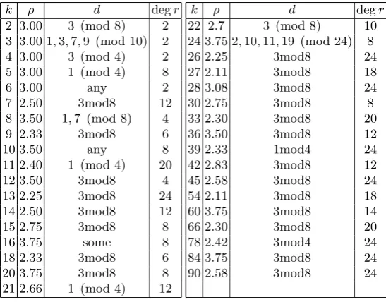
Table 1.Bestρ-values of complete families with variable discriminant ((r(x), π(x)) such that degr(x)<25, which are given in the appendix.
k ρ d degr
2 3.00 3 (mod 8) 2
3 3.00 1,3,7,9 (mod 10) 2
4 3.00 3 (mod 4) 2
5 3.00 1 (mod 4) 8
6 3.00 any 2
7 2.50 3mod8 12
8 3.50 1,7 (mod 8) 4
9 2.33 3mod8 6
10 3.50 any 8
11 2.40 1 (mod 4) 20
12 3.50 3mod8 4
13 2.25 3mod8 24
14 2.50 3mod8 12
15 2.75 3mod8 8
16 3.75 some 8
18 2.33 3mod8 6
20 3.75 3mod8 8
21 2.66 1 (mod 4) 12
k ρ d degr
22 2.7 3 (mod 8) 10
24 3.75 2,10,11,19 (mod 24) 8
26 2.25 3mod8 24
27 2.11 3mod8 18
28 3.08 3mod8 24
30 2.75 3mod8 8
33 2.30 3mod8 20
36 3.50 3mod8 12
39 2.33 1mod4 24
42 2.83 3mod8 12
45 2.58 3mod8 24
54 2.11 3mod8 18
60 3.75 3mod8 14
66 2.30 3mod8 20
78 2.42 3mod4 24
84 3.75 3mod8 24
90 2.58 3mod8 24
References
1. Barreto, P.S.L.M., Naehrig, M.: Pairing-friendly elliptic curves of prime order. In Selected Areas in Cryptography – SAC 2005. LNCS, vol. 3897, pp. 319-331. Springer, Heidelberg (2006)
2. Boneh, D., Franklin, M.: Identity-based encryption from the Weil pairing. In Advances in Cryptology Crypto 2001. LNCS, vol. 2139, pp. 213-229. Springer, Berlin (2001). Full version: SIAM J. Comput. 32(3), 586-615 (2003).
3. Boneh, D., Lynn, B., Shacham, H.: Short signatures from the Weil pairing. In Advances in Cryptology Asiacrypt 2001. LNCS, vol. 2248, pp. 514-532. Springer, Berlin (2002). Full version: J. Cryptol. 17, 297-319 (2004)
4. Brezing, F., Weng, A.: Elliptic curves suitable for pairing based cryptography. Des. Codes Cryptogr. 37, 133-141 (2005)
5. Cardona, G., Quer, J.: Field of moduli and field of definition for curves of genus 2. Available at: http://arxiv.org/abs/math/0207015.
6. Cardona, G., Quer, J.: Curves of genus 2 with group of automorphisms isomorphic to D8 or D12.
Trans. Amer. Math. Soc. 359, 2831-2849 (2007)
7. On constructing families of pairing-friendly elliptic curves with variable discriminant. INDOCRYPT-2011. LNCS, vol. 7107, pp. 310-319. Springer, Berlin (2011).
8. Freeman, D.: Constructing pairing-friendly elliptic curves with embedding degree 10. In Algorithmic Number Theory Symposium – ANTS-VII. LNCS, vol. 4076, pp. 452-465. Springer, Berlin (2006). 9. Freeman, D.: A generalized Brezing-Weng algorithm for constructing pairing-friendly ordinary abelian
varieties. In: Pairing-Based Cryptography – Pairing 2008. LNCS, vol. 5209, pp. 146-163. Springer, Heidelberg (2008)
10. Freeman, D., Satoh, T.: Constructing pairing-friendly hyperelliptic curves using Weil restriction. J. Number Theory 131, 959-983 (2011)
11. Freeman, D., Scott, M., Teske, E.: A taxonomy of pairing-friendly elliptic curves. J. Cryptol. 23, 224-280 (2010)
12. Freeman, D., Stevenhagen, P., Streng, M.: Abelian varieties with prescribed embedding degree. In: Algorithmic Number Theory – ANTS VIII. LNCS, vol. 5011, pp. 60-73. Springer, Heidelberg (2008) 13. Furukawa, E., Kawazoe, M., Takahashi, T.: Counting points for hyperelliptic curves of typey2=x5+ax
over finite prime fields. In Selected Areas in Cryptography – SAC 2003. LNCS, vol. 3006, pp. 26-41. Springer, Heidelberg (2004)
15. Galbraith, S., McKee, J., Valen¸ca, P.: Ordinary abelian varieties having small embedding degree. Finite Fields Appl. 13, 800–814 (2007)
16. Gaudry, P., Schost, E.: On the invariants of the quotients of the Jacobian of a curve of genus 2. In Applied Algebra, Algebraic Algorithms and Error-Correcting Codes — AAECC- 14. LNCS, vol. 2227, pp. 373-386. Springer, Heidelberg (2001)
17. Guillevic, A., Vergnaud, D.: Genus 2 Hyperelliptic Curve Families with Explicit Jacobian Order Eval-uation and Pairing-Friendly Constructions. To appear in Pairing-Based Cryptography – Pairing 2012, LNCS.
18. Howe, E., Zhu, H.: On the existence of absolutely simple abelian varieties of a given dimension over an arbitrary field. J. Number Theory 92, 139-163 (2002)
19. Igusa, J.: Arithmetic Variety of Moduli for Genus Two. Ann. Math. 72, 612-649 (1960)
20. Joux A.: A one round protocol for tripartite Diffie–Hellman. In Algorithmic Number Theory Sympo-sium – ANTS-IV. LNCS, vol. 1838, pp. 385-393. Springer, Berlin (2000). Full version: J. Cryptol. 17, 263-276 (2004)
21. Kachisa, E.: Generating More Kawazoe-Takahashi Genus 2 Pairing-Friendly Hyperelliptic Curves. In: Pairing-Based Cryptography – Pairing 2010. LNCS, vol. 6487, pp. 312-326. Springer, Heidelberg (2010).
22. Kachisa, E., Schaefer, E., Scott, M.: Constructing Brezing-Weng pairing friendly elliptic curves using elements in the cyclotomic field, inPairing-Based Cryptography–Pairing 2008. LNCS, vol. 5209, pp. 126-135. Springer, Heidelberg (2008)
23. Kawazoe, M., Takahashi, T.: Pairing-friendly ordinary hyperelliptic curves with ordinary Jacobians of typey2 =x5+ax. In: Pairing-Based Cryptography – Pairing 2008. LNCS, vol. 5209, pp. 164-177. Springer, Heidelberg (2008)
24. Lang, S.: Algebraic Number Theory. Graduate Texts in Mathematics, Vol. 110. Springer, Berlin (1994) 25. Miyaji, A., Nakabayashi, M., Takano, S.: New explicit conditions of elliptic curve traces for
FR-reduction. IEICE Trans. Fundam. E84-A(5), 1234–1243 (2001)
26. Milne, J.S.: Abelian varieties. In: Cornell, G., Silverman, J. (eds.) Arithmetic Geometry 103-150. Springer, New York (1986)
27. Murphy, A., Fitzpatrick, N.: Elliptic curves for pairing applications. Available at: http://eprint.iacr.org/2005/302
28. Maisner, D., Nart, E.: Abelian surfaces over finite fields as Jacobians. Experimental Mathematics 11, 321-337 (2002). With an appendix by Everett W. Howe.
29. Menezes, A., Okamoto, T., Vanstone, S.: Reducing elliptic curve logarithms to logarithms in a finite field. IEEE Trans. Inf. Theory 39, 1639-1646 (1993)
30. Mestre, J.F.: Construction de courbes de genre 2 `a partir de leurs modules. In Effective methods in algebraic geometry (Castiglioncello, 1990), pages 313-334. Birkh¨auser, Boston, MA (1991)
31. Rubin, K., Silverberg, A.: Using abelian varieties to improve pairing-based cryptography. J. Cryptol. 22, 330-364 (2009)
32. Scott, M., Barreto, P.S.L.M.: Generating more MNT elliptic curves. Des. Codes Cryptogr. 38, 209–217 (2006)
33. Shaska, T., Voelklein, H.: Elliptic subfields and automorphisms of genus 2 function fields. Algebra, arithmetic and geometry with applications (West Lafayette, IN, 2000), 703–723. Springer, Heidelberg (2004)
34. Silverman, J.: The Arithmetic of Elliptic Curves. Springer, Berlin (1986).
35. Sakai, R., Ohgishi, K., Kasahara, M.: Cryptosystems based on pairings. In 2000 Symposium on Cryp-tography and Information Security – SCIS 2000, Okinawa, Japan, 2000.
36. Sutherland, A.: Computing Hilbert class polynomials with the Chinese remainder theorem. Math. Comp. 80, 501-538 (2011)
37. Tate, J.: Classes d’isog´enie des vari´et´es ab´eliennes sur un corps fini. (d’apr´es T. Honda.) S´eminarie Bourbaki 1968/69, expos´e 352. Lect. Notes in Math., vol. 179, pp. 95-110. Springer (1971)
38. Tate, J.: Endomorphisms of abelian varieties over finite fields. Inventiones Mathematicae 2 (1966) 39. Waterhouse, W.C.: Abelian varieties over finite fields. Ann. Sci. ´Ecole Norm. Sup. 2, 521-560 (1969) 40. Waterhouse, W.C., Milne, J.S.: Abelian varieties over finite fields. Proc. Symp. Pure Math. 20, 53-64
9 Appendix: Complete families ((r(x), π(x)) with variable discriminant and best ρ-values such that degr(x) < 25.
k= 2, ρ= 3
r(x) =Φ6(x)
π(x) = ζ3
2 2x−1 +x
√ −x
k= 3, ρ= 3
r(x) =x2+ 11x+ 49
π(x) = ζ3
70 7x+ 56 + (x−17)
√ −x
k= 4, ρ= 3
r(x) =x2−6x+ 25
π(x) = 40i 5x+ 5 + (x+ 9)√−x
k= 5, ρ= 3
r(x) =Φ30(x)
π(x) = ζ3
2 −x6+x5+x−1−(x3+x2)
√ −x
k= 6, ρ= 3
r(x) =Φ6(x)
π(x) = ζ3
2 x−2 + (x−1)
√ −x
k= 7, ρ= 2.5
r(x) =Φ42(x)
π(x) = ζ3
2 x
7+x4−1 + (x7+x3−1)√−x
k= 8, ρ= 3.5
r(x) =x4+ 4x3+ 8x2−8x+ 4
π(x) = 24i −3x3−15x2−36x+ 6 + (x3+ 5x2+ 16x+ 2)√−x
k= 9, ρ= 2.33
r(x) =Φ18(x)
f1(x) = ζ23 x6−x3+ 1 + (x3+x2−1)
√ −x
k= 10, ρ= 3.5
r(x) =Φ30(5x)
π(x) = ζ3
k= 11, ρ= 2.4
r(x) =Φ66(x)
f1(x) = ζ23 −x12+x11+x−1 + (x6+x5)
√ −x
k= 12, ρ= 3.5
r(x) =Φ12(2x)
f1(x) = ζ23 −8x3+ 4x2−1 + (8x3−4x−1)
√ −x
k= 13, ρ= 2.25
r(x) =Φ78(x)
f1(x) = ζ3
2 x13−x7−1 + (x13−x6−1)
√ −x
k= 14, ρ= 2.5
r(x) =Φ42(x)
π(x) = ζ3
2 x
7−x4−1 + (−x7+x3+ 1)√−x
k= 15, ρ= 2.75
r(x) =Φ30(x)
f1(x) = ζ23 x5−x3−1 + (x5−x2−1)
√ −x
k= 16, ρ= 3.75
r(x) =x8+ 76x6+ 678x4+ 332x2+ 1
π(x) = 30464i 29x7−29x6+ 2173x5−2173x4+ 17175x3−17175x2−21009x+ 5777
+(5777x7−229x6+ 439081x5−17389x4+ 3918979x3−154335x2+ 1935139x
−71215)√−x
k= 18, ρ= 2.33
r(x) =Φ18(x)
π(x) = ζ3
2 x3−x2−1 + (−x3+x+ 1)
√ −x
k= 20, ρ= 3.75
r(x) =Φ20(2x)
π(x) = 2i −64x6+ 32x5+ 16x4−4x2+ 1 + (128x7−32x5−4x2−1)√−x
k= 21, ρ= 2.66
r(x) =Φ42(x)
π(x) = ζ3
2 −x
k= 22, ρ= 2.7
r(x) =Φ22(x)
π(x) = ζ3
2 x
11−x8−1 + (−x13+x5+x2)√−x
k= 24, ρ= 3.75
r(x) =x8+ 80x6+ 456x4+ 320x2+ 16
π(x) = ζ3
10752 −176x7+ 28x6−14040x5+ 2240x4−77088x3+ 12656x2−40480x+ 1792 +(177x7+ 34x6+ 14150x5+ 2704x4+ 79892x3+ 14248x2+ 50552x+ 9024)√−x
.
k= 26, ρ= 2.25
r(x) =Φ78(x)
π(x) = ζ3
2 x13+x7−1−(x13+x6−1)
√ −x
k= 27, ρ= 2.11
r(x) =Φ54(x)
π(x) = ζ3
2 x9−x5−1 + (−x9+x4+ 1)
√ −x
k= 28, ρ= 3.08
r(x) =Φ84(2x)
π(x) = ζ3
2 16384x
14−32x5−1 + (262144x18−131072x17+ 65536x16+ 32768x15
−4096x12−1024x10+ 64x6−4x2−1)√−x
k= 30, ρ= 2.75
r(x) =Φ30(x)
π(x) = ζ3
2 x
5+x3−1 + (−x5−x2+ 1)√−x
k= 33, ρ= 2.3
r(x) =Φ33(−x)
f1(x) = ζ23 x11+x6−1 + (x11+x5−1)
√ −x
k= 36, ρ= 3.5
r(x) =Φ36(2x)
f1(x) = ζ23 64x6−32x5−1 + (1024x10 + 512x9−128x7−16x4−1)
√ −x
k= 39, ρ= 2.33
r(x) =Φ78(x)
f1(x) = ζ3
2 −x14+x13+x−1−(x7+x6)
k= 42, ρ= 2.83
r(x) =Φ42(x)
π(x) = ζ3
2 x
7+x5−1x+ (x8+x3−x)√−x
k= 45, ρ= 2.58
r(x) =Φ90(x)
π(x) = ζ3
2 x
15+x8−1(x15+x7−1)√−x
k= 54, ρ= 2.11
r(x) =Φ54(x)
π(x) = ζ3
2 x9+x5−1 + (x9+x4−1)
√ −x
k= 60, ρ= 3.75
r(x) =Φ60(2x)
π(x) = ζ3
2 32768x
15+ 16384x14+ 4096x12−256x8−64x6−16x4+ 1
+(4096x12+ 1024x10−128x7+ 32x5−4x2−1)√−x
k= 66, ρ= 2.3
r(x) =Φ66(x)
π(x) = ζ3
2 x
11−x6−1 + (−x11+x5+ 1)√−x
k= 78, ρ= 2.42
r(x) =Φ78(x)
π(x) = ζ3
2 x
13−x8−1 + (x14−x6−x)√−x
k= 84, ρ= 3.75
r(x) =Φ84(2x)
π(x) = 12i
¯g(16384x
14+ 2x−1 + (−4194304x22−131072x17+ 65536x16−4096x12
−2048x11−1024x10+ 256x8+ 64x6+ 16x4−4x2−1)√−x
k= 90, ρ= 2.58
r(x) =Φ90(x)
f1(x) = 12 x15−x8−1 + (−x15+x7+ 1)
√ −x