Title: Scaling Based Active Contour Model in Grayscale Images

Available Online atwww.ijcsmc.com

International Journal of Computer Science and Mobile Computing

A Monthly Journal of Computer Science and Information Technology

ISSN 2320–088X

IMPACT FACTOR: 6.017

IJCSMC, Vol. 6, Issue. 5, May 2017, pg.293 – 300

Scaling Based Active Contour

Model in Grayscale Images

Zafer Guler

, Ahmet Cinar

¹Software Engineering Department & Firat University, Turkey

²Computer Engineering Department & Firat University, Turkey

1

[email protected]; 2 [email protected]

Abstract— Structures that can detect the shapes in images in a flexible manner are widely used today. Active contour model, which is one of these structures, is an important model. This model aims to surround the shape with points and to enable these points to fit into the shape. However, since Active Contour Model contains energy minimization, it requires long working time. Scaling based model developed in the present study proposed suggestions to solve speed problem of active contour model. Furthermore, this method allows working on the shape both outwardly (enlargement) and inwardly (reduction). Using the proposed model, conventional active contour model and developed (improved) active contour model (Gradient Vector Flow - GVF) were compared in terms of speed and the results were presented.

Keywords— Active Contour, Scaling, Gradient Vector Flow, Level Set, Snakes

I. INTRODUCTION

An image contains the useful information for a scientist. However, the image might not always be perceivable with the human eye only. It might be corrupted; might contain noise or its content might not be appropriate to serve our aims. In such cases, we have to use some techniques to distinguish the image and the information.

The first and most important step in image analysis is to segment the image. Segmentation refers to dividing the image into its components. In other words, the segmentation algorithm is the process of making the image black and white according to discontinuity and similarity properties in grayscale images [1]. One of the methods used in segmentation algorithm is based on sudden changes in grayscale. On the other hand, the second model is based on tresholding[2]. These methods only use the existing information in an image. The problems of these methods is that the edges are not only limited to the object. In controlled environments, excluding high-quality images, these methods produce spurious edges and gaps. Naturally, it is difficult to define and categorize spurious edges. These types of models are generally termed as low-level methods. [3].

this model impossible. In this case, adaptive techniques which can adjust itself according to the data and can find the appropriate result should be used. This is only possible by flexible shape formulations. Active contour model is one of the widely used models in flexible shape identification problems [3].

Active contour model had been widely used in a lot of application after it was proposed by Kass et al., and different approaches were developed for this approach [4]. The structure of active contour model is based on energy minimization procedure. Since this model contains many calculations, it has a low operation speed. The proposed model is based on extraction of shape without energy minimization like in active contour model. The structure of the paper is described below. Previous studies on active contour model were analysed in Chapter 2. Active contour model was analysed in Chapter 3. Application results of the developed model were presented in Chapter 4 and the obtained results were presented in Chapter 5.

II. PREVIOUS STUDIES

Active contour model has been widely used in many studies after it was proposed by Kass et al. in 1987. Various approaches were developed for the model. In 1992, active contour model was solved by Donna J. Williams and Mubarek Shan[5] using greedy algorithm and thus a speed increase was achieved. Furthermore, despite the strict limitations of dynamic programming, a better distribution of contour points was achieved maintaining stability and flexibility.

Gradient Vector Flow (GVF) which was developed by Chenyang Xu et al.,[6] in 1997 proposed solutions to the problems of the model. Thanks to calculated GVF force contour points allowed to find the shape even if it was very far. Shape can be successfully identified also in concave objects. However, GVF is expensive in terms of calculation and thus algorithm is slow. Geral Kühne et al., [7] proposed a semi-closed active contour based design in 2002. A significant speed increase was found in tests. Face contour was successfully and rapidly tracked using the algorithm developed by Xiong Bing et al.,[8] in 2004. The complexity of this algorithm is

. Where expresses number of contour points and expresses dimension of search window. Considering that search window is low, it is quite effective in reducing operation time. In 2005, Shin Jeongho et al., [9] proposed a new schema to extract contour and to track deformed objects. This procedure was achieved by adding motion estimation term to conventional active contour function. The proposed model requires less computation than the conventional method. Active contour model developed by Riadh Ksantini et al. [10] in 2009 aimed to improve polarity information which is purposed by Chunming et al. [11]. With using polarity information, visible object boundaries or edges in the image were obtained at a high accuracy. The method developed by Hongshe Dang et al,.[12] in 2009 is based on detection of the appropriate location using the algorithm (marker-based watershed algorithm) which use start contour required by geometric active contour method.. as a result, manual intervention was reduced and number of repetition on curve development was decreased. K. Manjusha et al., [13] developed, level set methods and non-linear diffusion equations based character segmentation algorithm in 2012. Level set methods were used in segmentation of written characters.

III.ACTIVE CONTOUR MODEL

Active Contour (snakes) model introduced a new approach to model feature extraction techniques. Active contour aims to surround the target feature [14]. These points are placed outside the target feature; the points are updated and approximated to the target feature. Steps in the procedure are presented in Fig. 1. In this sample, target feature is a vase. The first operation is to give contour points outside the vase Fig. 1 (a). Contour points are narrowed to a point close to the vase to detect the vase Fig. 1 (b, c, d, and e). (For this example each figure represent 75 loop.) Fig. 1 indicates that contour points have a good adaptation to the vase in Fig. 1 (f).

(d) (e) (f) Fig. 1 Identification of the shape using active contour [15].

Active contour is in fact the procedure of energy minimization. Target feature is the minimization of properly formulated energy function. Energy function is the sum of internal energy of the contour, constraint energy and image energy. These energies are indicated as , ve . These functions, which consist of points,

constitute the snake. Energy function is presented in the following equation [3].

∫ ( ) ( ) ( ) (1)

In this equation, internal energy controls natural behaviors of active contour and thus controls the order of the points. Image energy enables active contour to select low-level features such as edge points. On the

other hand, constraint energy uses high-level information to develop the contour. Active contour aims to

develop equation 2 by minimizing it. Low energy new contour points are better matched with target features and thus original points are developed [16].

Energy functions are expressed in unit of contour functions and image functions. These functions contribute to contour energy according to coefficients of selected related weights. As a result, internal energy of the image is defined as the sum of weighted first and second degree derivatives around the contour [17].

|

| |

| (2)

Internal energy controls flexibility and tension deformations of the conto+ur. The first-degree derivative measures energy caused by stretching and is represented as elastic energy [3]. The second-degree derivative measures energy caused by stretching and can also be expressed as curve energy. controls elastic energy coefficient, controls curve energy coefficient. Selection of and values enables us to control contour shape we aim to obtain. Small value means that difference between the points is not equally distributed. Similarly, great value means that difference between the points is equally distributed. Low value means failure of minimization of contour curve and formation of edges. Similarly, high values mean soft contour edges [3,6]. Above mentioned properties are the properties of the contour. We can reach a conclusion by comparing these properties with those of the shape.

Image energy enables the contour to identify low-level properties such as brightness or edge. Lines, edges and terminus contribute to energy function according to the original formula. The energy of these are indicated as , , and are controlled by , , weight coefficients respectively. Thus, image

energy is obtained as follows [3,18].

(3)

The formula of active contour method includes derivatives and the actual function of the method is to minimize equation 2. As a result, since the operations require much time, working speed is low [19,20,21]. For example, it is very difficult to apply active contour structure on video. The aim of the realized application is to learn how to accelerate a structure like active contour.

IV.DEVELOPED METHOD

Shape capture algorithms are based on the principle of an explicit color transition between the shape and the background. Thus, if one moves to the center of the shape from any point, edge of the shape can be detected with the intensity change in pixels. The first problem encountered here is lack of information about the shape and no information about the center of the shape. Another problem is concave property of the shape. In this case, as the coarse shaped pixel is approximated to the center, concentration on the outer edge can be explained by not stopping on the second edge in the inner side.

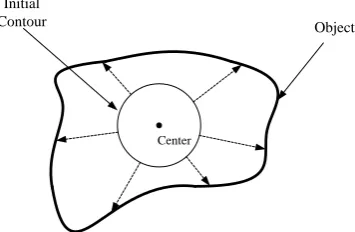
Sample object whose boundaries will be detected and initial contour are presented in Fig. 2 and 3. As indicated in the figures, the application can work both outwardly and inwardly. The direction (inward or outward) and speed of initial contour is determined by scaling coefficient. Scaling coefficient is selected as smaller than 1 to achieve outward reduction of initial contour. Making the number smaller enables faster movement of the contour; while making it closer to 1 enables contour to move more slowly. Scaling coefficient is selected smaller than 1 to ensure that initial contour grows outwardly; on the other hand, increase of this number means fast contour while being close to 1 ensures slow movement of the contour. In this developed application, scaling coefficient was selected as 0.95 in reduction and 1.05 in enlargement. Movement samples of initial contour are presented in Fig. 2 and Fig. 3 To perform scaling process, we should know object center; in other words, which point we should take as a basis to perform scaling. Since we don’t have previous knowledge about the object in the present study, the center is the arithmetic mean of contour points. Fig. 2 and Fig. 3 represent the situations which contain relatively smooth boundaries. As we see, there will be no problem in detecting the object and the object will be extracted successfully. However, when we want to extract a concave object, the algorithm will not yield a successful result and it will fail to detect internal sections of the object. Fig. 4 gives general structure of the proposed algorithm.

Initial Contour

Object

Center

Fig. 2 Image of coarse shape and object – Reduction

Initial

Contour _Object

Center

Fig. 3 Image of coarse shape and object - Enlargement

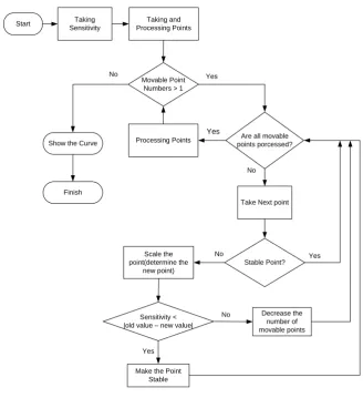
movement of the contour; while making it closer to 1 enables contour to move more slowly. Scaling coefficient is selected smaller than 1 to ensure that initial contour grows outwardly; on the other hand, increase of this number means fast contour while being close to 1 ensures slow movement of the contour. In this developed application, scaling coefficient was selected as 0.95 in reduction and 1.05 in enlargement. Movement samples of initial contour are presented in Fig. 2 and Fig. 3. To perform scaling process, we should know object center; in other words, which point we should take as a basis to perform scaling. Since we don’t have previous knowledge about the object in the present study, the center is the arithmetic mean of contour points. Fig. 2 and Fig. 3 represent the situations which contain relatively smooth boundaries. As we see, there will be no problem in detecting the object and the object will be extracted successfully. However, when we want to extract a concave object, the algorithm will not yield a successful result and it will fail to detect internal sections of the object. Fig. 4 gives general structure of the proposed algorithm.

One of the important operations in the flow chart presented in Fig. 4 is to take sensitivity variable. It is possible to define this variable as the density difference between the object and the background. Its function is to inform that there is an edge if the value between two pixels is greater than sensitivity value; and to inform that there is no edge if the value is smaller than the sensitivity value. This value can vary from image to image and according to the shape that is to be detected and thus the users are enable to use this function.

Are all movable points porcessed?

Scale the point(determine the

new point)

Sensitivity < |old value – new value|

Make the Point Stable

No

Yes

No Taking and

Processing Points

Take Next point

Stable Point?

No Yes

Movable Point Numbers > 1

Yes

Finish No Start _SensitivityTaking

Processing Points

Yes

Decrease the number of movable points Show the Curve

Fig. 4 Flow chart of the proposed model

Fig. 5 Pseudo code of the developed model

Complexity of the developed algorithm is . number dynamically shows variation in the program. It decreases when reduction is applied; increases when enlargement is applied.

V. APPLICATIONS

In this study, an alternative method was developed for active contour model. Using the developed model, speed problem of the active contour method was tried to be solved with a scaling based approach. The method was applied in computer media and results were taken by applying to various images. Sample image of the application is presented in Fig. 6.

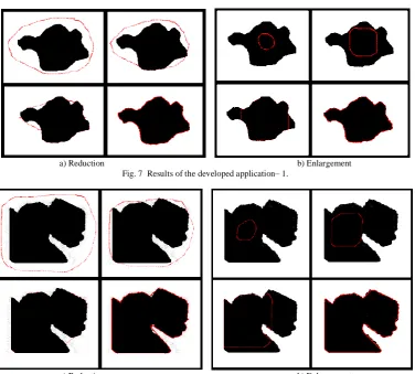
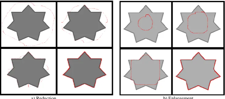
Using the developed model, the procedure of extracting the object can be performed much more rapidly than active contour model. The results obtained from the developed model are presented in Fig. 7 and Fig. 8. Shape detection rates were calculated by taking into account known real boundary points and detected boundary points. For example, the image in Fig. 7 contains 109200 pixels (400x273) and the object contains 22373 pixels. The developed model finds 22130 pixels, so for this image our model can find 99% of the object.

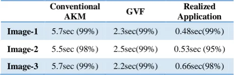
The images in Fig. 7, 8 and 9 were tested with conventional active contour model applied by Ritwik[15] and “active contour model with Gradient Vector Flow” developed by Chenyang Xu et al,.[6] and using the developed model, working time and detection rate of the shape were compared in percentages. The results are presented in Table 1. As indicated in Table 1, a great increase was achieved in terms of working time and similar success rates were obtained. The test was performed in Microsoft Visual Studio 2010 media. The features of the used computer are presented below.

• Intel(R) Core(TM) i5 CPU M 560 @ 2,67GHz • 4 GB DDR3 Ram

• ATI Mobility Redeon HD 5650 Graphic Card

TABLE I

COMPARISON OF APPLICATION Conventional

AKM GVF

Realized Application Image-1 5.7sec (99%) 2.3sec(99%) 0.48sec(99%)

Image-2 5.5sec (98%) 2.5sec(99%) 0.53sec (95%)

Image-3 5.7sec (99%) 2.2sec(99%) 0.66sec(98%)

Enter: d {sensitivity}, n {number of points},serie[n] {contour points}

ns <-- Numberofpoint() {Number of movable points}

{All points at the beginning}

sbt[] <-- Stabile() {Stabile points}

{Blank at the beginning}

while ns>1

center <-- average(serie) for i=0 to n

if !sbt[i] {If the point is not stabile}

yn <-- scaling (serie[i], center) if d<difference(serie[i]-yn) sbt[i] <-- stabile ns <-- ns - 1

correct() {arrangement of points}

Fig. 6 Sample image of the developed application

a) Reduction b) Enlargement

Fig. 7 Results of the developed application– 1.

a) Reduction b) Enlargement

a) Reduction b) Enlargement

Fig. 9 Results of the developed application – 3.

VI.CONCLUSION

In this study, a scaling based approach was found for active contour models. Using only geometric scaling matrix, with enlargement and reduction procedures, object boundaries were captured at an accuracy of 98%. The use of convex objects increased accuracy. Future studies will work on an adaptive structure for both concave and convex objects. We plan to apply the model on parallel structures for the situations which require simultaneous working using more than one object.

R

EFERENCES

[1] W. Juang, K. Zheng, and X. Zhu, “Gray-Level Image Segmentation based on Markov Chain Monte Carlo”, Educational Technology and Computer Science, ETCS ’09. vol. 2, pp 279-282, 2009.

[2] A.K.C. Wong, P.K. Sahoo, “A Gray-level Threshold selection method based on Maximum Entropy Principle”, Systems, Man and Cybernetics, IEEE Transactions, vol. 19, pp. 866-871, 1989.

[3] N. Kokrmaz, “A Software Development for Spinal Deformity Analysis and Diagnosis”, PhD Thesis, Marmara University Institute of Science, Department of Electronics and Computer Education, İstanbul, 2008.

[4] M. Kass, A. Witkin ve D. Terzopoulos, Snakes: Active Contour Model, International Journal of Computer Vision, vol. 1, no. 4, pp. 321-331, 1988.

[5] D. J. Williams, M. Shah, “A Fast Algorithm for Active Contour and Curvature Estimation”, CVGIP: Image Understanding, vol. 55, pp. 14-26, 1992.

[6] C, Xu and J.L. Prince, “Gradient Vector Flow: A New External Force for Snakes,” Proc. IEEE Conf. on Comp. Vis. Patt. Recog. (CVPR), pp. 66-71, 1997.

[7] G. Kühne, J. Weickert, M. Beier, W. Effrlsberg, “Fast Implicit Active Contour Models”, Pattern Recognition, vol. 2449, pp. 133-140, 2002.

[8] X.Bing, Y. Wei and C. Charoensak, “Face Contour Tracking in Video Using Active Contour Model”, Image Processing, ICIP’04, pp. 1021-1024, 2004.

[9] J. Shin, H. Ki, J. Paik, “Motion-Based Hierarchical Active Contour Model for Deformable Object Tracking”, Computer Analysis of Images and Patterns, vol. 3691, pp. 806-813, 2005.

[10] R. Ksantini, F. Shariat ve B. Boufama, “An Efficient and Fast Active Contour Model for Salient Object Detection”, Computer and robot Vision (CRV), pp. 124-131, 2009.

[11] C. Li, C. Xu, C. Gui, M.D. Fox, “Level set evolution withoud re-initialization: a new variational formulation”, Computer Vision and Pattern Recognition, vol. 1, pp. 430-436, 2005.

[12] H. Dang, Y. Hong, X. Fang, F. Qiang, “Initial Contour Automatic Selection of Geometric Active Contour Model”, Second International Conference on Intelligent Computation Technology and Automation, pp. 66-69, 2009.

[13] K. Manjusha, S. Sachin Kumar, J. Rajendran, K. P. Soman, “Hindi Character Segmentation in Document Images Using Level Set Methods and Non-linear Diffusion”, International Journal of Computer Applications(0975-8887), vol. 44, pp. 44-49, 2012.

[14] V.A. Atılı ve İ. Bayram, “Image Segmentation with Global Active Contours”, Signal Processing and Communication Applications Conference (SIU), pp. 1-4, 2012.

[15] K, Ritwik., (2010), Snakes: Active Contour Model. [Online]. Available: https://www.mathworks.com/matlabcentral/fileexchange/28109-snakes--active-contour-models

[16] M. S. Nixon, A.S. Agunda, Feature Extraction and Image Processing, Newnes, First Edition, 2002. [17] S. Osher ve R. Fedkiw, Level Set Methods and Dynamic Implicit Surfaces. Springer, 2003.

[18] H. Dang, Y. Hong, X. Fang ve F. Qiang, “Initial Contour Automatic Selection of Geometric Active Contour Model”, Intelligent Computation Technology and Automation, pp. 66-69, 2009.

[19] R. Ksantini, F. Shariat ve B. Boufama, “An Efficient and Fast Active Contour Model for Salient Object Detection”, Computer and robot Vision (CRV), pp. 124-131, 2009.

[20] M. Niethammer, A. Tannenbaum, S. Angenent, “Dynamic active Contours for Visual Tracking”, IEEE Transactions on automatic Kontrol, pp. 562-579, 2006.