Comparison of Mamdani and Sugeno Fuzzy Inference System Models for Resonant Frequency Calculation of Rectangular Microstrip Antennas

(1)

COMPARISON OF MAMDANI AND SUGENO FUZZY INFERENCE SYSTEM MODELS FOR RESONANT FREQUENCY CALCULATION OF RECTANGULAR MICROSTRIP ANTENNAS

K. Guney

Department of Electrical and Electronics Engineering Faculty of Engineering

Erciyes University Kayseri 38039, Turkey

N. Sarikaya

Department of Aircraft Electrical and Electronics Civil Aviation School

Erciyes University Kayseri 38039, Turkey

Abstract—Models based on fuzzy inference systems (FISs) for

calculating the resonant frequency of rectangular microstrip antennas (MSAs) with thin and thick substrates are presented. Two types of FIS models, Mamdani FIS model and Sugeno FIS model, are used to compute the resonant frequency. The parameters of FIS models are determined by using various optimization algorithms. The resonant frequency results predicted by FIS models are in very good agreement with the experimental results available in the literature. When the performances of FIS models are compared with each other, the best result is obtained from the Sugeno FIS model trained by the least-squares algorithm.

(2)

1. INTRODUCTION

MSAs have many desirable features such as low proﬁle, light weight, conformal structure, low production cost, and ease of integration with microwave integrated circuit or monolithic microwave integrated circuit components [1–5]. MSAs are therefore used extensively in a broad range of commercial and military applications.

In MSAdesigns, it is important to determine the resonant frequencies of the antenna accurately because MSAs have narrow bandwidths and can only operate effectively in the vicinity of the resonant frequency. So, a technique to compute accurately the resonant frequency is helpful in antenna designs. Several techniques [1–39] are available in the literature to calculate the resonant frequency of rectangular MSA, as this is one of the most popular and convenient shapes. These techniques can be broadly classified into two categories: analytical and numerical techniques. The analytical techniques offer both simplicity and physical insight, but depend on several assumptions and approximations that are valid only for thin substrates. The numerical techniques provide accurate results but usually require considerable computational time and costs.

The neural models trained by various algorithms were used in calculating the resonant frequency of rectangular MSAs [26, 28, 29, 31]. Aneuro-fuzzy network was presented in [30] to compute the resonant frequencies of MSAs. In [30], the number of rules and the premise parameters of Sugeno FIS were determined by the fuzzy subtractive clustering method and then the consequent parameters of each output rule were determined by using linear least squares estimation method. The training data sets were obtained by numerical simulations using a moment-method code based on electric ﬁeld integral equation approach. To validate the performances of the neuro-fuzzy network, a set of further moment-method simulations was realized and presented to the neuro-fuzzy network.

(3)

nonlinear systems capable of inferring complex nonlinear relationships between input and output data. The high-speed real-time computation feature of the FIS recommends its use in antenna computer aided design (CAD) programs.

In previous works [27, 33–35, 44–50], we successfully used Sugeno FISs for computing accurately the various parameters of the rectangular, triangular, and circular MSAs. In [27, 33], the tabu search algorithms and the hybrid learning algorithm were used to train the Sugeno FISs. However, in this paper, six diﬀerent optimization algorithms, least-squares (LSQ) algorithm [51–53], nelder-mead (NM) algorithm [54, 55], genetic algorithm (GA) [56, 57], diﬀerential evolution algorithm (DEA) [58–60], particle swarm optimization (PSO) [61, 62], and simulated annealing (SA) algorithm [63–65], are used to train the Sugeno FISs. Furthermore, in this paper, Mamdani FIS models trained by LSQ, NM, GA, DEA, PSO, and SA are proposed to compute the resonant frequency of rectangular MSAs.

2. FIS MODELS FOR RESONANT FREQUENCY COMPUTATION

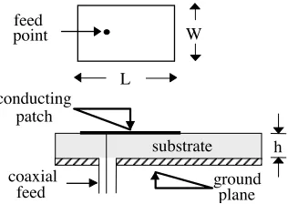
Figure 1 shows a rectangular patch of width W and length L over a ground plane with a substrate of thickness h and a relative dielectric constantεr. Asurvey of the literature [1–39] clearly shows that only

four parameters,W,L,h, andεr, are needed to describe the resonant

frequency. In this paper, the resonant frequency of the rectangular MSAis computed by using FIS models. The FIS is a very powerful approach for building complex and nonlinear relationship between a set of input and output data [40–43].

ground plane conducting

patch

substrate h

coaxial feed feed

point W

L

Figure 1. Geometry of rectangular MSA.

(4)

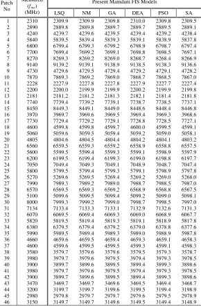
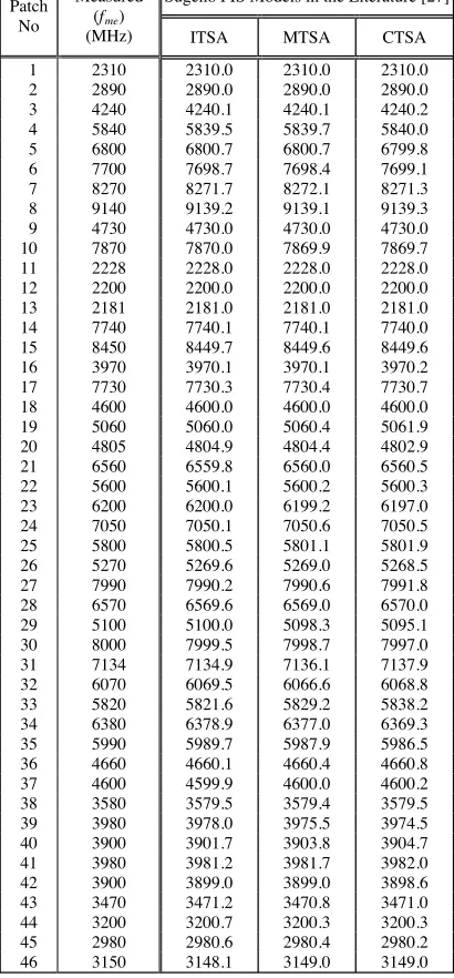
Table 1. Measured resonant frequency results and dimensions for electrically thin and thick rectangular MSAs.

Patch No

W (cm)

L (cm)

h

(cm) εr (h/λd)x100

Measured ( fme)

(MHz) 1 5.700 3.800 0.3175 2.33 3.7317 2310+ 2 4.550 3.050 0.3175 2.33 4.6687 2890+ 3 2.950 1.950 0.3175 2.33 6.8496 4240+ 4 1.950 1.300 0.3175 2.33 9.4344 5840+ 5* 1.700 1.100 0.3175 2.33 10.9852 6800+ 6 1.400 0.900 0.3175 2.33 12.4392 7700+ 7 1.200 0.800 0.3175 2.33 13.3600 8270+ 8 1.050 0.700 0.3175 2.33 14.7655 9140+ 9 1.700 1.100 0.9525 2.33 22.9236 4730+ 10 1.700 1.100 0.1524 2.33 6.1026 7870+ 11 4.100 4.140 0.1524 2.50 1.7896 2228∆ 12* 6.858 4.140 0.1524 2.50 1.7671 2200∆ 13 10.800 4.140 0.1524 2.50 1.7518 2181∆ 14 0.850 1.290 0.0170 2.22 0.6535 7740 15* 0.790 1.185 0.0170 2.22 0.7134 8450 16 2.000 2.500 0.0790 2.22 1.5577 3970 17 1.063 1.183 0.0790 2.55 3.2505 7730 18 0.910 1.000 0.1270 10.20 6.2193 4600 19 1.720 1.860 0.1570 2.33 4.0421 5060 20* 1.810 1.960 0.1570 2.33 3.8384 4805 21 1.270 1.350 0.1630 2.55 5.6917 6560 22 1.500 1.621 0.1630 2.55 4.8587 5600 23* 1.337 1.412 0.2000 2.55 6.6004 6200 24 1.120 1.200 0.2420 2.55 9.0814 7050 25 1.403 1.485 0.2520 2.55 7.7800 5800 26 1.530 1.630 0.3000 2.50 8.3326 5270 27 0.905 1.018 0.3000 2.50 12.6333 7990 28 1.170 1.280 0.3000 2.50 10.3881 6570 29* 1.375 1.580 0.4760 2.55 12.9219 5100 30 0.776 1.080 0.3300 2.55 14.0525 8000 31 0.790 1.255 0.4000 2.55 15.1895 7134 32 0.987 1.450 0.4500 2.55 14.5395 6070 33* 1.000 1.520 0.4760 2.55 14.7462 5820 34 0.814 1.440 0.4760 2.55 16.1650 6380 35 0.790 1.620 0.5500 2.55 17.5363 5990 36 1.200 1.970 0.6260 2.55 15.5278 4660 37 0.783 2.300 0.8540 2.55 20.9105 4600 38* 1.256 2.756 0.9520 2.55 18.1413 3580 39 0.974 2.620 0.9520 2.55 20.1683 3980 40 1.020 2.640 0.9520 2.55 19.7629 3900 41 0.883 2.676 1.0000 2.55 21.1852 3980 42 0.777 2.835 1.1000 2.55 22.8353 3900 43 0.920 3.130 1.2000 2.55 22.1646 3470 44* 1.030 3.380 1.2810 2.55 21.8197 3200 45 1.265 3.500 1.2810 2.55 20.3196 2980 46 1.080 3.400 1.2810 2.55 21.4787 3150

+_{These frequencies measured by Chang et al. [14].}∆_{These frequencies}

(5)

differences between these three FISs lie in the consequents of their fuzzy rules, and thus their aggregation and defuzzification procedures differ accordingly. In this paper, Mamdani and Sugeno FIS models are used to calculate accurately the resonant frequency of rectangular MSAs. The data sets used in training and testing Mamdani and Sugeno FIS models have been obtained from the previous experimental works [8, 14, 22, 23], and are given in Table 1. The 37 data sets in Table 1 are used to train the FISs. The 9 data sets, marked with an asterisk in Table 1, are used for testing. For the FIS models, the inputs areW,L,h, andεrand the output is the measured resonant frequency

fme.

In this paper, the grid partitioning method [41] is used for the fuzzy rule extraction. In the grid partitioning method, the domain of each antecedent variable is partitioned into equidistant and identically shaped membership functions (MFs). Amajor advantage of the grid partitioning method is that the fuzzy rules obtained from the ﬁxed linguistic fuzzy grids are always linguistically interpretable. Using the available input-output data, the parameters of the MFs can be optimized.

In this paper, the number of MFs for the input variables W, L, h, and εr are determined as 3, 3, 2, and 3, respectively. Each possible

combination of inputs and their associated MFs is represented by a rule in the rule base of the Mamdani and Sugeno FIS models. So, the number of rules for FIS models is 54 (3×3×2×3 = 54).

The application of the Mamdani and Sugeno FIS models to the resonant frequency calculation is given in the following sections.

2.1. Mamdani FIS Modelsfor Resonant Frequency Computation

(6)

M11 M12 M13 M21 M22 M23 M31 M32 M41 M42 M43 1 54 2 53 27

1 o1 ;o1, o1

Z M z c σ

2 o2 ;o2, o2

Z M z c

27 o27 ;o27, o27

Z M z c

53 o53 ;o53, o53

Z M z c

54 o54 ;o54, o54

Z M z c

1Z1

53Z53 2Z2

54Z54 27Z27

54 ω 1 ω W L h r me O f Layer #1 Fuzzy Layer Layer #2 Product Layer Layer #3 Implication Layer Layer #4 Aggregation Layer 2 ω 27 ω 53 ω o M Layer #5 De-fuzzy Layer σ σ σ σ ω ω ω ω ω ε Π Π Π Π U ∫ = = = = = ( ) ( ) ( ) ( ) ( ) Π

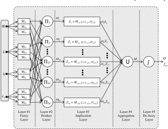
Figure 2. Architecture of Mamdani FIS for resonant frequency

computation of rectangular MSA.

an adaptive node. The rule base for Mamdani FIS can be written as

1. if (W isM11) and (L isM21) and (h isM31) and (εr isM41)

thenZ1 =Mo1(z;co1, σo1)

4. if (W isM11) and (L isM21) and (h isM32) and (εr isM41) (1)

..

. ...

thenZ53=Mo53(z;co53, σo53)

(7)

with

Zk =Mok(z;cok, σok) k= 1, . . . ,54 (2)

where Mij, Zk, and Mok represent the jth MF of the ith input, the

output of thekth rule, and thekth output MF, respectively. In Eq. (1), cokandσokare the consequent parameters that characterize the shapes

of the output MFs.

As shown in Figure 2, the Mamdani FIS architecture consists of ﬁve layers: fuzzy layer, product layer, implication layer, aggregation layer, and de-fuzzy layer. Layered operating mechanism of the Mamdani FIS can be described as follows:

Layer 1: In this layer, the crisp input values are converted to the fuzzy values by the input MFs. In this paper, the following generalized bell, trapezoidal, and gaussian MFs for the inputs are used:

i) Generalized bell MFs for (i= 1 or i= 4), (j= 1,2,3), (x=W or x=εr):

Mij(x) =Gbell(x;aij, bij, cij) =

1

1 +x−cij aij

2bij

(3a)

ii) Trapezoidal MFs for i= (2), j = (1,2,3), (x=L):

Mij(x) =T rap(x;aij, bij, cij, dij) =                   

0, x≤aij

x−aij

bij−aij

, aij ≤x≤bij

1, bij ≤x≤cij

dij −x

dij −cij

, cij ≤x≤dij

0, dij ≤x

(3b)

iii) Gaussian MFs for (i= 3),(j= 1,2), (x=h):

Mij(x) =Gauss(x;cij, σij) =e −1

2

x−cij σij

2

(3c)

where aij, bij, cij, dij, and σij are the premise parameters that

characterize the shapes of the input MFs.

Layer 2: In this layer, the weighting factor (ﬁring strength) of each rule is computed. The weighting factor of each rule, which is expressed as ωk, is determined by evaluating the membership

(8)

the input MFs in the layer 1 and then applying the “and” operator to these membership values. The “and” operator corresponds to the multiplication of input membership values. Hence, the weighting factors of the rules are computed as follows:

ω1 =M11(W)M21(L)M31(h)M41(εr)

ω2 =M11(W)M21(L)M31(h)M42(εr)

ω3 =M11(W)M21(L)M31(h)M43(εr)

ω4 =M11(W)M21(L)M32(h)M41(εr)

..

. ...

ω53=M13(W)M23(L)M32(h)M42(εr)

ω54=M13(W)M23(L)M32(h)M43(εr)

(4)

Layer 3: In this layer, the implication of each output MF is computed by

Mimp,k =ωkZk k= 1, . . . ,54 (5)

whereMimp,k represents the implicated output MFs.

Layer 4: In this layer, the aggregation is performed to produce an overall output MF,Mo(z), by using the union operator:

Mo(z) = 54

k=1

Mimp,k = 54

k=1

ωkZk

=

54

k=1

ωkMok(z;cok, σok) = 54

k=1

ωke−

1 2

_z₋_cok

σok

2

(6)

The types of the output MFs (Mok) are Gaussian. Here, the “union”

operation is performed using the maximum operator.

Layer 5: In this layer, the defuzziﬁcation is performed by using the centroid of area method:

O=

Z

Mo(z) z dz

Z

Mo(z)dz

(7)

(9)

M11 M12 M13 M21 M22 M23 M31 M32 M41 M42 M43 1 54 2 53 27 N1 N54 N2 N53 N27

1 1,1 1,2 1,3 1,4r 1,5 Z=p W+p L+p h+p +p

2 2,1 2,2 2,3 2,4r 2,5 Z =p W p L+p h+ p +p

27 27,1 27,2 27,3 27,4 r 27,5 Z =p W +p L +p h+p +p

53 53,1 53,2 53,3 53,4r 53,5 Z =p W +p L+p h+p +p

54 54,1 54,2 54,3 54,4r 54,5 Z =p W +p L +p h+ p +p

1Z1

2

27

53

54

53Z53 2Z2

54Z54 27Z27 1

W L h r

54 1 W L h r Layer #1 Fuzzy Layer Layer #2 Product Layer Layer #3 Normalized Layer Layer #4 De-Fuzzy Layer Layer #5 Summation Layer me O f

W L h r

ω ε Π Π Π Π Π ω ω ω ω ω ε ε ε ε ε ω ω ω ω ω Σ + ω ε ε ε ε ε

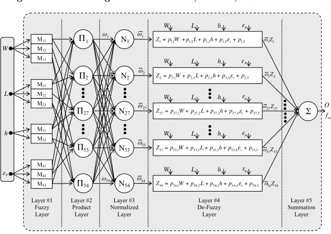
Figure 3. Architecture of Sugeno FIS for resonant frequency

computation of rectangular MSA.

2.2. Sugeno FIS Modelsfor Resonant Frequency Computation

Sugeno FIS [41, 42] was proposed to develop a systematic approach to generate fuzzy rules from a given input-output data. The Sugeno FIS architecture used in this paper for the resonant frequency calculation is shown in Figure 3. The rule base for Sugeno FIS is given by

1. if (W isM11) and (LisM21) and (h isM31) and (εr isM41)

thenZ1 =r1(W, L, h, εr)

4. if (W isM11) and (LisM21) and (h isM32) and (εr isM41) (8)

..

(10)

thenZ53=r53(W, L, h, εr)

thenZ54=r54(W, L, h, εr)

with

Zk =rk(W, L, h, εr) k= 1, . . . ,54 (9)

where Mij, Zk, and rk represent the jth MF of the ith input, the

output of thekth rule, and the kth output MF, respectively.

As shown in Figure 3, the Sugeno FIS structure consists of ﬁve layers: fuzzy layer, product layer, normalized layer, de-fuzzy layer, and summation layer. It is clear thatLayer 1and Layer 2of Sugeno FIS are the same as those of Mamdani FIS. The operating mechanism of the other layers for Sugeno FIS can be described as follows:

Layer 3: The normalized weighting factor of each rule, ¯ωk, is

computed by using

¯ ωk =

ωk 54 i=1

ωi

k= 1, . . . ,54 (10)

Layer 4: In this layer, the output rules can be written as:

¯

ωkZk = ¯ωkrk(W, L, h, εr)

= ¯ωk(pk1W +pk2L+pk3h+pk4εr+pk5) k= 1, . . . ,54 (11)

where pk are the consequent parameters that characterize the shapes

of the output MFs. Here, the types of the output MFs (rk) are linear.

Layer 5: Each rule is weighted by own normalized weighting

factor and the output of the FIS is calculated by summing of all rule outputs:

O=

54

k=1

¯ ωkZk=

54 k=1

ωkZk

54 k=1

ωk

(12)

(11)

Table 2. Comparison of measured and calculated resonant frequencies obtained by using Mamdani FIS models presented in this paper for electrically thin and thick rectangular MSAs.

Present Mamdani FIS Models Patch

No

Measured (fme)

(MHz) LSQ NM GA DEA PSO SA

(12)

Table 3. Comparison of measured and calculated resonant frequencies obtained by using Sugeno FIS models presented in this paper for electrically thin and thick rectangular MSAs.

Present Sugeno FIS Models Patch

No

Measured (fme)

(MHz) LSQ NM GA DEA PSO SA

(13)

Table 4. Resonant frequencies obtained from the Sugeno FIS models available in the literature for electrically thin and thick rectangular MSAs.

Sugeno FIS Models in the Literature [27] Patch

No

Measured (fme)

(MHz) ITSA MTSA CTSA

(14)

Table 5. Resonant frequencies obtained from the conventional methods available in the literature for electrically thin and thick rectangular MSAs.

Conventional Methods in the Literature Patch

No

Measured (fme)

(15)

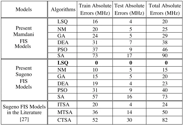
Table 6. Train, test, and total absolute errors between the measured and calculated resonant frequencies for FIS models.

Models Algorithms Train Absolute

Errors (MHz)

Test Absolute Errors (MHz)

Total Absolute Errors (MHz)

LSQ 16 4 20

NM 20 5 25

GA 24 5 29

DEA 31 7 38

PSO 37 9 46

Present Mamdani

FIS Models

SA 73 17 90

LSQ 0 0 0

NM 10 5 15

GA 15 5 20

DEA 19 4 23

PSO 31 9 40

Present Sugeno

FIS Models

SA 57 16 73

ITSA 20 4 24

MTSA 36 14 50

Sugeno FIS Models in the Literature

[27] CTSA 52 30 82

Table 7. Total absolute errors between the measured and calculated resonant frequencies for the conventional methods.

Conventional Methods in the Literature

[6] [7] [8] [1] [2] [11]

Errors (MHz) 36059 26908 1104916 19179 32930 23746 Conventional

Methods in the Literature

[15] [16] [19] [23] [23] [32]

Errors (MHz) 23761 19899 31436 108707 126945 10132

2.3. Determination of Design Parameters of Mamdani and Sugeno FIS Models

(16)

algorithms, LSQ, NM, GA, DEA, PSO, and SA, are used to determine the optimum values of the design parameters and adapt the FISs. Basic optimization framework steps of these algorithms for the calculation of resonant frequency by using Mamdani and Sugeno FIS models are summarized below:

Step 1: Choose the initial FIS structure. In this step, the number and the types of MFs for the input variablesW, L, h,andεrare found.

Thus, the numbers of the premise parameters (aij, bij, cij,dij, andσij)

and the consequent parameters (cok and σok or pk) are determined.

Learning Error Inputs

(W, L, h,

ε

r)

FIS

Target Output (fme)

Optimization Algorithm

+

Output (fr)

Σ

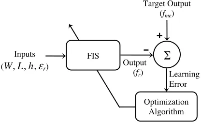
-Figure 4. FIS model for calculating the resonant frequency.

Step 2: Initialize the values of the premise and consequent parameters. Initial values of the premise and consequent parameters are produced. Hence, the input MFs are equally spaced and made to cover the universe of discourse.

Step 3: Compute the output (resonant frequency fr). FIS

produces the output (fr) for a given input data (W, L, h, and εr)

using the premise and the consequent parameters in the inference mechanism.

Step 4: Evaluate the performance of FIS. The learning error between the target (measured resonant frequencyfme) and the actual

output is computed. In this paper, mean square error (MSE) criterion is used for this purpose.

Step 5: Continue or terminate the process. In this step,

termination criterion of the optimization algorithm is checked. If the learning error is equal to/small from the predetermined error value or iterations reach to a ﬁnal value, the process is stopped. Otherwise, the process continues to Step 6.

Step 6: Update the parameter values using the optimization

(17)

-0.1 0.1 0.3 0.5 0.7 0.9 0

0.2 0.4 0.6 0.8 1 1.2 1.4 1.6

Input Range

Membership Value

input #1, gbell MF#1 input #1, gbell MF#2 input #1, gbell MF#3

-0.1 0.1 0.3 0.5 0.7 0.9 0

0.2 0.4 0.6 0.8 1 1.2 1.4 1.6

Input Range

Membership Value

input #2, trap MF#1 input #2, trap MF#2 input #2, trap MF#3

-0.1 0.1 0.3 0.5 0.7 0.9

0 0.2 0.4 0.6 0.8 1 1.2 1.4 1.6

Input Range

Membership Value

input #3, gauss MF#1 input #3, gauss MF#2

-0.1 0.1 0.3 0.5 0.7 0.9

0 0.2 0.4 0.6 0.8 1 1.2 1.4 1.6

Input Range

Membership Value

input #4, gbell MF#1 input #4, gbell MF#2 input #4, gbell MF#3

Figure 5. Shapes of the MFs of input variables (Input #1 =W, Input #2 =L, Input #3 =h, and Input #4 =εr) for the Sugeno FIS model

trained by the LSQ.

DEA, PSO, and SA) is used for updating the values of the premise and the consequent parameters so as to decrease the learning error. Then, the process continues from Step 3.

The process explained above is simply given in Figure 4.

3. RESULTS AND CONCLUSIONS

(18)

Tables 4 and 5, respectively. ITSA, MTSA, and CTSA in Table 4 represent, respectively, the resonant frequencies calculated by the Sugeno FIS models trained by the improved tabu search algorithm (ITSA), the modified tabu search algorithm (MTSA), and the classical tabu search algorithm (CTSA). The resonant frequency results in twelfth and thirteenth columns of Table 5 are obtained by using the curve-fitting formula [23] and by using the modified cavity model [23], respectively. The sum of the absolute errors between the theoretical and experimental results for FIS models and conventional methods is listed in Tables 6 and 7.

When the performances of Mamdani and Sugeno FIS models are compared with each other, the best result is obtained from the Sugeno FIS model trained by the LSQ algorithm, as shown in Tables 2, 3, 4 and 6. The ﬁnal shapes of the input MFs are illustrated in Figure 5 for the Sugeno FIS model trained by the LSQ algorithm. For brevity, the ﬁnal shapes of the MFs of other FIS models are not given.

It is clear from Tables 5 and 7 that the conventional methods [1, 2, 6–8, 11, 15, 16, 19, 23, 32] give comparable results. Some cases are in very good agreement with measurements, and others are far oﬀ. When the results of FIS models are compared with the results of the conventional methods, the results of all FIS models are better than those predicted by the conventional methods. The very good agreement between the measured resonant frequency values and the computed resonant frequency values of FIS models supports the validity of the FIS models and also illustrates the superiority of FIS models over the conventional methods.

In this paper, the FIS models are trained and tested with the experimental data taken from the previous experimental works [8, 14, 22, 23]. It is clear from Tables 5 and 7 that the theoretical resonant frequency results of the conventional methods are not in very good agreement with the experimental results. For this reason, the theoretical data sets obtained from the conventional methods are not used in this work. Only the measured data set is used for training and testing the FIS models.

(19)

REFERENCES

1. Bahl, I. J. and P. Bhartia, Microstrip Antennas, Artech House, Dedham, MA, 1980.

2. James, J. R., P. S. Hall, and C. Wood,Microstrip Antennas-theory and Design, Peter Peregrisnus Ltd., London, 1981.

3. Bhartia, P., K. V. S. Rao, and R. S. Tomar, Millimeter-wave Microstrip and Printed Circuit Antennas, Artech House, Canton, MA, 1991.

4. Pozar, D. M. and D. H. Schaubert, Microstrip Antennas — The

Analysis and Design ofMicrostrip Antennas and Arrays, IEEE

Press, New York, 1995.

5. Garg, R., P. Bhartia, I. Bahl, and A. Ittipiboon, Microstrip

Antenna Design Handbook, Artech House, Canton, MA, 2001.

6. Howell, J. Q., “Microstrip antennas,” IEEE Trans. Antennas Propagat., Vol. 23, 90–93, 1975.

7. Hammerstad, E. O., “Equations for microstrip circuits design,”

Proceedings ofthe 5th European Microwave Conference, 268–272, Hamburg, 1975.

8. Carver, K. R., “Practical analytical techniques for the microstrip antenna,” Proceedings ofthe Workshop on Printed Circuit

Antenna Tech., 7.1–7.20, New Mexico State University, Las

Cruces, 1979.

9. Richards, W. F., Y. T. Lo, and D. D. Harrison, “An improved theory for microstrip antennas and applications,” IEEE Trans. Antennas Propagat., Vol. 29, 38–46, 1981.

10. Bailey, M. C. and M. D. Deshpande, “Integral equation formulation of microstrip antennas,” IEEE Trans. Antennas Propagat., Vol. 30, 651–656, 1982.

11. Sengupta, D. L., “Approximate expression for the resonant frequency of a rectangular patch antenna,” Electronics Lett., Vol. 19, 834–835, 1983.

12. Pozar, D. M., “Considerations for millimeter wave printed antennas,” IEEE Trans. Antennas Propagat., Vol. 31, 740–747, 1983.

13. Mosig, J. R. and F. E. Gardiol, “General integral equation formulation for microstrip antennas and scatterers,” IEE Proc. Microwaves, Antennas Propagat., Vol. 132, 424–432, 1985. 14. Chang, E., S. A. Long, and W. F. Richards, “An experimental

in-vestigation of electrically thick rectangular microstrip antennas,”

(20)

15. Garg, R. and S. A. Long, “Resonant frequency of electrically thick rectangular microstrip antennas,”Electronics Lett., Vol. 23, 1149– 1151, 1987.

16. Chew, W. C. and Q. Liu, “Resonance frequency of a rectangular microstrip patch,” IEEE Trans. Antennas Propagat., Vol. 36, 1045–1056, 1988.

17. Damiano, J. P. and A. Papiernik, “A simple and accurate model for the resonant frequency and the input impedance of printed antennas,” Int. J. Microwave Millimeter-wave Computer-aided Eng., Vol. 3, 350–361, 1993.

18. Verma, A. K. and Z. Rostamy, “Resonant frequency of uncovered and covered rectangular microstrip patch using modiﬁed Wolﬀ model,”IEEE Trans. Microwave Theory Tech., Vol. 41, 109–116, 1993.

19. Guney, K., “Anew edge extension expression for the resonant frequency of electrically thick rectangular microstrip antennas,”

Int. J. Electronics, Vol. 75, 767–770, 1993.

20. Guney, K., “Resonant frequency of a tunable rectangular microstrip patch antenna,”Microwave Opt. Technol. Lett., Vol. 7, 581–585, 1994.

21. Lee, I. and A. V. Vorst, “Resonant-frequency calculation for electrically thick rectangular microstrip patch antennas using a dielectric-looded inhomogeneous cavity model,” Microwave Opt. Technol. Lett., Vol. 7, 704–708, 1994.

22. Kara, M., “The resonant frequency of rectangular microstrip antenna elements with various substrate thicknesses,”Microwave Opt. Technol. Lett., Vol. 11, 55–59, 1996.

23. Kara, M., “Closed-form expressions for the resonant frequency of rectangular microstrip antenna elements with thick substrates,”

Microwave Opt. Technol. Lett., Vol. 12, 131–136, 1996.

24. Mythili, P. and A. Das, “Simple approach to determine resonant frequencies of microstrip antennas,” IEE Proc. Microwaves, Antennas Propagat., Vol. 145, 159–162, 1998.

25. Ray, K. P. and G. Kumar, “Determination of the resonant frequency of microstrip antennas,”Microwave Opt. Technol. Lett., Vol. 23, 114–117, 1999.

26. Karaboga, D., K. Guney, S. Sagiroglu, and M. Erler, “Neural computation of resonant frequency of electrically thin and thick rectangular microstrip antennas,” IEE Proc. Microwaves, Antennas Propagat., Vol. 146, 155–159, 1999.

(21)

frequency of electrically thin and thick rectangular microstrip antennas with the use of fuzzy inference systems,”Int. J. RF and Microwave Computer-aided Eng., Vol. 10, 108–119, 2000.

28. Guney, K., S. Sagiroglu, and M. Erler, “Comparison of neural networks for resonant frequency computation of electrically thin and thick rectangular microstrip antennas,” Journal of

Electromagnetic Waves and Applications, Vol. 15, 1121–1145,

2001.

29. Guney, K., S. Sagiroglu, and M. Erler, “Generalized neural method to determine resonant frequencies of various microstrip antennas,” Int. J. RF and Microwave Computer-aided Eng., Vol. 12, 131–139, 2002.

30. Angiulli, G. and M. Versaci, “Resonant frequency evaluation of microstrip antennas using a neural-fuzzy approach,”IEEE Trans. Magnetics, Vol. 39, 1333–1336, 2003.

31. Guney, K. and S. S. Gultekin, “Artiﬁcial neural networks for resonant frequency calculation of rectangular microstrip antennas with thin and thick substrates,” Int. J. Infrared and Millimeter Waves, Vol. 25, 1383–1399, 2004.

32. Guney, K., “Anew edge extension expression for the resonant frequency of rectangular microstrip antennas with thin and thick substrates,” J. Communications Tech. and Electronics, Vol. 49, 49–53, 2004.

33. Guney, K. and N. Sarikaya, “Adaptive neuro-fuzzy inference system for computing the resonant frequency of electrically thin and thick rectangular microstrip antennas,” Int. J. Electronics, Vol. 94, 833–844, 2007.

34. Guney, K. and N. Sarikaya, “Ahybrid method based on combining artiﬁcial neural network and fuzzy inference system for simultaneous computation of resonant frequencies of rectangular, circular, and triangular microstrip antennas,” IEEE Trans. Antennas Propagat., Vol. 55, 659–668, 2007.

35. Guney, K. and N. Sarikaya, “Concurrent neuro-fuzzy systems for resonant frequency computation of rectangular, circular, and triangular microstrip antennas,” Progress In Electromagnetics Research, PIER 84, 253–277, 2008.

36. Akdagli, A., “An empirical expression for the edge extension in calculating resonant frequency of rectangular microstrip antennas with thin and thick substrates,”Journal ofElectromagnetic Waves and Applications, Vol. 21. 1247–1255, 2007.

(22)

antennas,” Progress In Electromagnetics Research B, Vol. 8, 77– 86, 2008.

38. Tokan, N. T. and F. Gunes, “Support vector characterization of the microstrip antennas based on measurements,” Progress In Electromagnetics Research B, Vol. 5, 49–61, 2008.

39. Ray, I., M. Khan, D. Mondal, and A. K. Bhattacharjee, “Eﬀect on resonant frequency for E-plane mutually coupled microstrip antennas,”Progress In Electromagnetics Research Letters, Vol. 3, 133–140, 2008.

40. Mamdani, E. H. and S. Assilian, “An experiment in linguistic synthesis with a fuzzy logic controller,” Int. J. Man-machine Studies, Vol. 7, 1–13, 1975.

41. Jang, J.-S. R., C. T. Sun, and E. Mizutani,Neuro-fuzzy and Soft Computing: A Computational Approach to Learning and Machine Intelligence, Prentice-Hall, Upper Saddle River, NJ, 1997.

42. Takagi, T. and M. Sugeno, “Fuzzy identiﬁcation of systems and its applications to modeling and control,” IEEE Trans. Systems, Man, and Cybernetics, Vol. 15, 116–132, 1985.

43. Jang, J.-S. R., “ANFIS: Adaptive-network-based fuzzy inference system,” IEEE Trans. Systems, Man, and Cybernetics, Vol. 23, 665–685, 1993.

44. Kaplan, A., K. Guney, and S. Ozer, “Fuzzy associative memories for the computation of the bandwidth of rectangular microstrip antennas with thin and thick substrates,” Int. J. Electronics, Vol. 88, 189–195, 2001.

45. Guney, K. and N. Sarikaya, “Adaptive neuro-fuzzy inference system for the input resistance computation of rectangular microstrip antennas with thin and thick substrates,” Journal of Electromagnetic Waves and Applications, Vol. 18, 23–39, 2004. 46. Guney, K. and N. Sarikaya, “Computation of resonant frequency

for equilateral triangular microstrip antennas using adaptive neuro-fuzzy inference system,” Int. J. RF and Microwave Computer-aided Eng., Vol. 14, 134–143, 2004.

47. Guney, K. and N. Sarikaya, “Adaptive neuro-fuzzy inference system for computing the resonant frequency of circular microstrip antenna,” The Applied Computational Electromagnetics Society J., Vol. 19, 188–197, 2004.

(23)

49. Guney, K. and N. Sarikaya, “Multiple adaptive-network-based fuzzy inference system for the synthesis of rectangular microstrip antennas with thin and thick substrates,” Int. J. RF and Microwave Computer-aided Eng., Vol. 18, 359–375, 2008.

50. Guney, K. and N. Sarikaya, “Adaptive-network-based fuzzy inference system models for input resistance computation of circular microstrip antennas,” Microwave Opt. Technol. Lett., Vol. 50, 1253–1261, 2008.

51. Levenberg, K., “Amethod for the solution of certain nonlinear problems in least-squares,”Quart. Appl. Math. II, 164–168, 1944. 52. Marquardt, D. W., “An algorithm for least-squares estimation of nonlinear parameters,” SIAM J. Appl. Math., Vol. 11, 431–441, 1963.

53. Dennis, J. E., State ofthe Art in Numerical Analysis, Academic Press, 1977.

54. Spendley, W., G. R. Hext, and F. R. Himsworth, “Sequential application of simplex designs in optimization and evolutionary operation,”Technometrics, Vol. 4, 441–461, 1962.

55. Nelder, J. A. and R. Mead, “A simplex method for function minimization,” Computer J., Vol. 7, 308–313, 1965.

56. Holland, J., Adaptation in Natural and Artiﬁcial Systems, University of Michigan Press, MI, 1975.

57. Goldberg, D. E.,Genetic Algorithms in Search, Optimization and Machine Learning, Addison-Wesley, Reading, MA, 1989.

58. Price, K. V., “Diﬀerential evolution: Afast and simple numerical optimizer,” 1996 Biennial Conference of the North American Fuzzy Information Processing Society, 524–527, Berkeley, CA, 1996.

59. Storn, R. M. and K. V. Price, “Diﬀerential evolution: Asimple and eﬃcient heuristic for global optimization over continuous spaces,” J. Global Opt., Vol. 11, 341–359, 1997.

60. Price, K. V., R. M. Storn, and J. Lampinen, Diﬀerential Evolution: A Practical Approach to Global Optimization, Springer, Berlin, 2005.

61. Kennedy, J. and R. Eberhart, “Particle swarm optimization,”

Proceedings ofthe IEEE Int. Conference on Neural Networks,

1942–1948, Perth, Australia, 1995.

62. Eberhart, R. and J. Kennedy, “Anew optimizer using particle swarm theory,” Proceedings ofthe Sixth International

Symposium on Micro Machine and Human Science, 39–43,

(24)

63. Metropolis, N., A. W. Rosenbluth, M. N. Rosenbluth, A. H. Teller, and E. Teller, “Equations of state calculations by fast computing machines,”J. Chemical Physics, Vol. 21, 1087–1092, 1953. 64. Pincus, M., “AMonte Carlo method for the approximation

solution of certain types of constrained optimization problems,”

Operations Research, Vol. 18, 1225–1228, 1970.