Length Sensing and Control of a Prototype Advanced
Interferometric Gravitational Wave Detector
Thesis by
Robert L. Ward
In Partial Fulfillment of the Requirements
for the Degree of
Doctor of Philosophy
California Institute of Technology
Pasadena, California
2010
c
2010 Robert L. Ward
Acknowledgements
First and foremost, I would like to thank my advisor, Alan Weinstein. His guidance was invaluable,
and if I learned anything during this process, it was that whenever we argued, he would turn out to
be right. It is not possible to describe in words the debt I owe to Rana Adhikari. By example, he
showed me how to think, what to measure, and how to enjoy the process. Thanks for everything.
Many thanks to Osamu Miyakawa, who first showed me how to not blind myself with a laser, Seiji
Kawamura who gave me my first lesson in control theory, and to Steve Vass, who has always been,
and always will be, a true pleasure to work with. Sam Waldman showed me how the perfect is the
enemy of actually finishing something. Stefan Ballmer graciously let me take over the radiometer.
Matt Evans and Hartmut Grote both helped tremendously during critical periods. Thanks also
go to all my other friends and colleagues at the 40 m, for making it such a great place to work:
Bob Taylor, John Miller, Yoichi Aso, Koji Arai, Jenne Driggers, Kirk McKenzie, Bram Slagmolen,
Kiwamu Izumi, Alberto Stochino, Joe Betzweiser, and Tobin Fricke. Then there’s David
Yeaton-Massey, Aidan Brooks, Zack Korth, and Alastair Heptonstall, who never let me write in peace.
The CDS crew, Ben and Rich Abbott, Rolf Bork, Jay Heefner, and Alex Ivanov, was invaluable.
Without their support, nothing at the 40 m would have ever worked. Thanks to Mike Smith for his
help with the OMC.
My family has always been supportive, and I especially want to thank my parents for always
letting me do whatever I wanted.
My most excellent friends at Caltech deserve much blame for the length of this work. They
made this place too much fun to leave. The usual suspects were Dan, Brad, Christie, James,
Keiko, Andrew, Meredith, John, Spanish Jon, Jack, Lindsey, Dylan, Emily, Jan, Katerina, Kirk,
Ella, Tommy, and Nicola. They and all the other Friends of the BWMA made Pasadena home.
Everybody always had a good time, and nobody ever got hurt.
And of course, Marie-H´el`ene. You really are the center of the universe.
Finally the boilerplate: LIGO was constructed by the California Institute of Technology and
Mas-sachusetts Institute of Technology with funding from the National Science Foundation and operates
under cooperative agreement PHY-0757058. This work was also supported by the NSF Graduate
Abstract
There is a worldwide effort to directly detect gravitational radiation. The Laser Interferometer
Gravitational Wave Observatory (LIGO) operates three kilometer-scale interferometric gravitational
wave detectors at two sites: two in Hanford, WA and one in Livingston, LA. A significant upgrade,
called Advanced LIGO, is planned for these detectors. The core work of this thesis involves using
a 40 m prototype interferometer on the Caltech campus to study length and sensing and control
techniques for Advanced LIGO. The principal results are the development of a lock acquisition
protocol for an advanced detector and a comparison of noise couplings between two gravitational
wave signal extraction techniques, called RF and DC readout.
In addition, a search in LIGO data was carried out for broadband, long-duration stochastic
Contents
Acknowledgements iii
Abstract iv
1 Introduction 1
2 Gravitational Waves 3
2.1 Gravity . . . 3
2.2 Gravitational Waves . . . 5
2.2.1 The Evidence: PSR B1913+16 . . . 6
2.3 Sources of Gravitational Waves and Detection Strategies . . . 6
2.3.1 The Stochastic Background of Graviational Radiation . . . 6
2.3.2 Continuous Wave Sources . . . 7
2.3.3 Compact Binary Coalesences . . . 8
2.3.4 Unmodeled Short-Duration Sources . . . 8
2.4 Gravitational Wave Detection . . . 8
2.4.1 Terrestrial Gravitational Wave Detectors . . . 9
2.4.1.1 Resonant Mass Antenna. . . 9
2.4.1.2 Optical Interferometers . . . 9
2.5 LIGO . . . 10
2.5.1 The LIGO Scientific Collaboration . . . 10
2.6 A New Window on the Universe . . . 11
3 Interferometeric Gravitational Wave Detection 12 3.1 Principle of Operation . . . 12
3.2 Noise. . . 13
3.3 Mathematical Notations for Mirrors, Fields, and Spaces . . . 15
3.4 The Michelson Interferometer as a Gravitational Wave Detector. . . 17
3.5.1 Optical Heterodyne Detection. . . 20
3.5.1.1 Schnupp Asymmetry for Michelson Length Sensing . . . 22
3.5.2 Optical Homodyne Detection . . . 23
3.6 Fabry-P´erot Cavities . . . 23
3.6.1 Cavity Spatial Modes . . . 25
3.6.2 Transfer Functions of a Fabry-P´erot Cavity . . . 27
3.6.3 The Pound-Drever-Hall Technique . . . 28
3.7 Adding Fabry-P´erot Cavities to the Arms of a Michelson Interferometer . . . 30
3.8 Coupled Cavities . . . 31
3.8.1 Antiresonant Short Cavity. . . 32
3.8.2 Resonant Short Cavity. . . 33
3.8.3 Detuned Short Cavity . . . 33
3.9 Recycling . . . 35
3.9.1 Power Recycling . . . 35
3.9.2 Signal Recycling . . . 37
3.10 Resonant Sideband Extraction . . . 38
3.11 Detuned RSE . . . 39
3.11.1 Two-Photon Formalism . . . 39
3.11.2 The RSE Response Function . . . 40
3.11.3 Detuned RSE Interferometers as Optical Springs . . . 42
3.11.3.1 Dynamical Instability . . . 43
3.11.3.2 Anti-spring . . . 43
3.11.4 The Detuned Resonant Sideband Extraction Interferometer with Power Recy-cling . . . 44
3.12 Feedback Control . . . 44
3.12.0.1 Noise reduction . . . 46
3.12.0.2 Transduction linearity . . . 46
3.13 The Advanced LIGO Design. . . 46
4 Gravitational Wave Signal Extraction 49 4.1 RF Readout. . . 50
4.2 DC Readout. . . 51
4.3 Considerations . . . 51
4.3.1 Laser Noise Couplings . . . 52
4.3.2 Spatial Overlap . . . 54
4.3.3.1 OMC noise mechanisms . . . 54
4.3.4 Oscillator Noise. . . 55
4.3.4.1 Oscillator amplitude noise . . . 55
4.3.4.2 Oscillator phase noise . . . 56
4.3.5 Flicker Noise . . . 56
4.3.6 Unsuppressed Signal . . . 56
4.3.7 Shot Noise . . . 57
4.3.8 Signal Linearity. . . 57
4.4 Decision . . . 57
5 The Caltech 40 m Prototype Interferometer 59 5.1 Prototyping . . . 59
5.2 Vacuum and Seismic Isolation. . . 61
5.3 Suspensions . . . 61
5.4 Electronics and Digital Controls . . . 62
5.5 Pre-Stabilized Laser . . . 63
5.5.1 MOPA. . . 63
5.5.2 Power Stabilization. . . 64
5.5.3 Frequency Stabilization . . . 64
5.5.4 Pre-Mode Cleaner . . . 65
5.6 Input Optics . . . 65
5.6.1 Phase Modulations . . . 65
5.6.1.1 A Mach-Zehnder interferometer for non-cascaded RF sidebands . . 65
5.6.2 Input Mode Cleaner . . . 66
5.6.3 Input Isolation, Mode Matching, and Steering. . . 66
5.7 The Common Mode Servo . . . 67
5.8 Interferometer. . . 67
5.9 Output Optics . . . 67
5.9.1 Output Mode Cleaner . . . 69
5.9.1.1 OMC Length Sensing and Control . . . 69
5.9.2 Output Steering . . . 69
5.9.3 Output Mode Matching . . . 69
5.9.4 Higher Order Mode Content at Asymmetric Port . . . 71
5.9.5 Photodetectors . . . 71
6 The Length Sensing and Control Scheme 73
6.1 Principle. . . 73
6.2 Resonance Profile. . . 74
6.3 Sensing . . . 76
6.3.1 Signal Selection: Ports, Frequencies, and Quadratures . . . 76
6.3.2 Double Demodulation . . . 76
6.3.3 Sideband Imbalance and Offsets . . . 77
6.3.3.1 Measuring Demodulation Phases . . . 77
6.3.4 Configuration Space and the Operating Point . . . 79
6.3.5 Discriminants . . . 79
6.3.5.1 Frequency dependence. . . 80
6.3.5.2 Position dependence . . . 82
6.3.5.3 Example matrix at operating point . . . 82
6.3.5.4 SPOB . . . 83
6.3.5.5 Non-resonant sideband . . . 83
6.4 Control . . . 83
6.4.1 Matrices and Bases. . . 84
6.4.1.1 Input Matrix . . . 86
6.4.2 Feedforward Corrections . . . 86
6.5 Discussion . . . 87
7 Calibration of a Detuned RSE Interferometer 89 7.1 Calibration in Initial LIGO . . . 89
7.1.1 Free Swinging Michelson. . . 90
7.1.2 ITM Calibration . . . 90
7.1.3 ETM Calibration . . . 91
7.1.4 DARM calibration . . . 91
7.1.4.1 Tracking . . . 91
7.1.4.2 Comment . . . 92
7.2 Calibrating the 40 m Detuned RSE Interferometer . . . 92
7.2.1 Actuator Calibration . . . 92
7.2.2 DARM Calibration. . . 93
7.2.3 Modeling . . . 94
7.2.4 Tracking. . . 95
8 Lock Acquisition 100
8.1 Lock Acquisition: The Path to Control. . . 100
8.2 Lock Acquisition of a Resonant Cavity . . . 101
8.2.1 Threshold velocity . . . 101
8.2.2 Normalized PDH locking . . . 102
8.2.3 Loop Triggering . . . 102
8.2.4 Offset locking . . . 102
8.3 Lock Acquisition of Coupled Cavities. . . 103
8.3.1 Lock Acquisition for Initial LIGO and Virgo . . . 104
8.4 Lock Acquisition of a Detuned Resonant Sideband Extraction Interferometer with Power Recycling . . . 105
8.5 Bootstrapping. . . 105
8.5.1 Interferometer subsets . . . 105
8.5.2 Alignment. . . 106
8.5.3 Double Demodulation signals . . . 107
8.6 The Lock Acquisition Procedure for the Caltech 40 m Interferometer . . . 108
8.6.1 Initial Acquisition . . . 108
8.6.2 The spring and the anti-spring . . . 110
8.6.2.1 Locking the spring and the anti-spring. . . 110
8.6.3 The Protocol . . . 112
8.6.4 Adaptive compensation filter: the moving zero . . . 116
8.6.5 Other Protocols. . . 119
8.6.6 Scripting Tools . . . 121
8.7 Deterministic Locking . . . 121
8.7.1 The Future: It’s easy being green. . . 123
8.7.1.1 Envisioned lock acquisition procedure . . . 124
8.7.1.2 Advantages of this technique . . . 125
8.7.1.3 Alternative Technique . . . 125
8.8 Discussion . . . 126
9 Measurement of Laser and Oscillator Noise Couplings in RF/DC Readout 127 9.1 DC Readout Experiment. . . 127
9.1.1 Noise Injections. . . 128
9.1.1.1 Laser Amplitude Noise . . . 128
9.1.1.2 Laser Frequency Noise. . . 128
9.2 Power Recycled Fabry-P´erot Michelson Interferometer . . . 129
9.2.1 Simulation . . . 129
9.2.2 Laser Amplitude Noise. . . 130
9.2.2.1 DC Readout . . . 130
9.2.2.2 RF Readout . . . 130
9.2.3 Laser Frequency Noise . . . 131
9.2.4 Oscillator Phase Noise . . . 131
9.2.5 Oscillator Amplitude Noise . . . 133
9.3 Detuned RSE Interferometer . . . 135
9.3.1 Length Offsets . . . 135
9.3.1.1 Cyclical dependencies . . . 135
9.3.1.2 Mode cleaner length . . . 136
9.3.1.3 Effect on DARM calibration . . . 136
9.3.2 Simulation . . . 136
9.3.2.1 Feedback and Offsets . . . 137
9.3.3 The simulated noise traces. . . 137
9.3.3.1 Effects not included . . . 138
9.3.3.2 Auxiliary loop coupling . . . 138
9.3.4 Laser Amplitude Noise. . . 138
9.3.4.1 DC Readout . . . 138
9.3.4.2 RF Readout . . . 139
9.3.5 Laser Frequency Noise . . . 140
9.3.5.1 DC Readout . . . 140
9.3.5.2 RF Readout . . . 141
9.3.6 Oscillator Phase Noise . . . 141
9.3.6.1 DC Readoutf1. . . 142
9.3.6.2 DC Readoutf2. . . 142
9.3.6.3 RF Readoutf1 . . . 143
9.3.6.4 RF Readoutf2 . . . 143
9.3.7 Oscillator Amplitude Noise . . . 144
9.3.7.1 DC Readoutf1. . . 144
9.3.7.2 DC Readoutf2. . . 145
9.3.7.3 RF Readoutf1 . . . 145
9.3.7.4 RF Readoutf2 . . . 145
10 A Directional Cross-Correlation Search for Stochastic Gravitational Waves Using
Data from the Fifth LIGO Science Run 150
10.1 Stochastic Gravitational Waves . . . 150
10.2 Detecting stochastic gravitational waves . . . 151
10.2.1 Isotropic strategy. . . 152
10.2.2 Segmenting Data and Optimal Combination. . . 153
10.2.3 Gravitational Wave Radiometry . . . 155
10.2.4 The Point Spread Function . . . 156
10.3 Analysis Pipeline . . . 156
10.4 Limits on Gravitational Waves . . . 158
10.4.1 Detection . . . 158
10.4.2 The Data . . . 161
10.4.3 Data Quality . . . 161
10.4.3.1 Frequency Masking . . . 161
10.4.3.2 Delta-Sigma Cut . . . 161
10.4.4 Posterior Distributions and Upper Limits . . . 162
10.4.5 Gravitational Wave SkyMap . . . 164
10.4.5.1 Injection . . . 164
10.5 Frequency and Location Resolved Searches . . . 165
10.5.1 Upper Limit on gravitational waves from Sco X1 . . . 165
10.5.2 The Galactic Center . . . 166
10.5.3 Globular Clusters. . . 167
10.5.4 Untargeted Narrowband Search on the Whole Sky . . . 175
10.5.5 Injection. . . 175
10.6 Future Work . . . 176
10.6.1 Detection Thresholding . . . 176
10.6.2 Multi-baseline Radiometry . . . 177
10.6.3 Transient Searches . . . 177
10.6.4 Clustering . . . 178
10.7 Discussion . . . 178
11 Summary and Conclusion 179
A Acronyms 181
C Laser Noise Coupling Formulae 187
C.1 Asymmetries and Couplings . . . 187
C.2 Laser noise coupling to asymmetric port . . . 187
D Resonant Cavity Formulae 195 D.1 Statics . . . 195
D.2 Equilibrium Frequency Response . . . 196
D.3 Coupled Cavities . . . 198
E Feedback 200 E.1 Linear Control: Loopology. . . 200
E.2 Servo Stability . . . 202
E.2.1 Bode gain-phase relationship . . . 202
E.2.2 Conditional Stability . . . 202
E.3 Servo Bandwidth . . . 203
E.4 Feedback Filter Design . . . 203
E.4.1 MIMO control . . . 203
E.4.1.1 Cross Coupling. . . 205
F Interferometer Modeling 206 F.1 Modeling Tools . . . 206
F.1.1 FINESSE . . . 206
F.1.2 GWINC . . . 206
F.1.3 Optickle . . . 207
F.1.4 Looptickle. . . 207
F.1.5 E2E: End to End . . . 207
F.1.6 FFT . . . 207
F.2 MATLAB code . . . 208
F.2.1 The RSE response function . . . 208
List of Figures
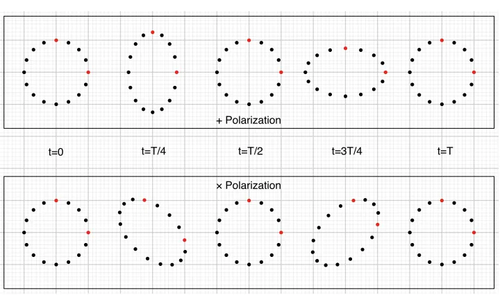
2.1 Effect of a GW on a circle of test particles. . . 7
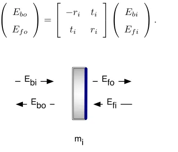
3.1 Input and output fields of a mirror mass. . . 16
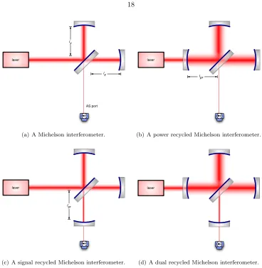
3.2 Michelson based interferometer topologies for gravitational wave detection. . . 18
3.3 A Fabry-P´erot Cavity with overlapping waves. . . 25
3.4 Cavity gain vs. bandwidth. . . 29
3.5 A schematic of a typical PDH length sensing setup . . . 29
3.6 The PDH signals for a single cavity. . . 30
3.7 A three mirror coupled cavity. . . 31
3.8 Effect of adding a third mirror with a short cavity on the bandwidth of the coupled system. . . 33
3.9 A Power Recycled Fabry-P´erot Michelson Interferometer. . . 36
3.10 A Dual Recycled Fabry-P´erot Michelson Interferometer. . . 38
3.11 Changing the detuning of the signal cavity . . . 42
3.12 Frequency response in different readout quadratures . . . 43
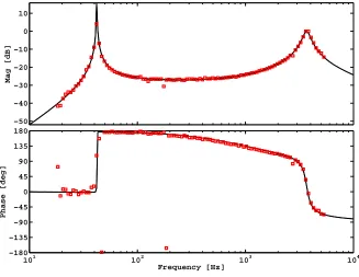
3.13 Measurement of the opto-mechanical RSE response. . . 44
3.14 Measurement of the opto-mechanical RSE response in an anti-spring configuration . . 45
3.15 Projected sensitivity for possible operating modes of Advanced LIGO. . . 48
4.1 Phasor diagram of the asymmetric port in an RF readout scheme. . . 50
4.2 Phasor diagram of the asymmetric port in a DC readout scheme. . . 52
5.1 The layout of the 40 m. . . 60
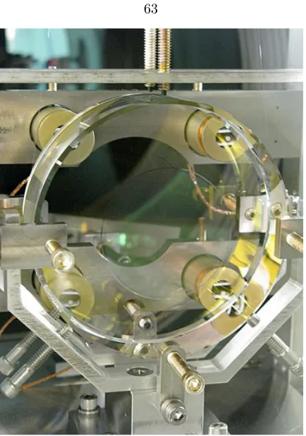
5.2 A MOS suspension. . . 63
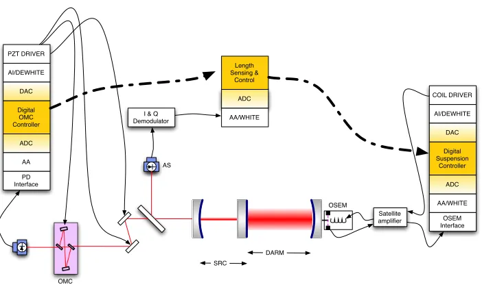
5.3 Real time control network example. . . 64
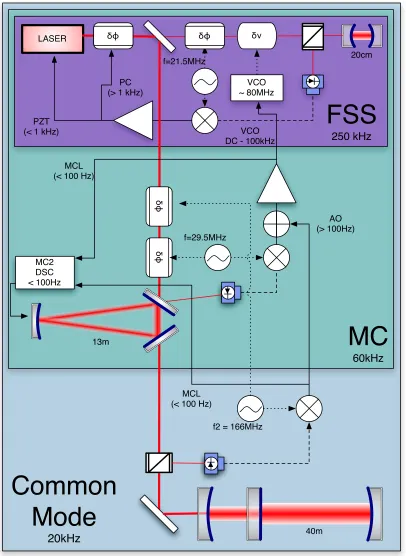
5.4 The laser frequency stabilization system. . . 68
5.5 An example EPICS control screen . . . 70
5.6 Mode scans of the AS port . . . 72
6.1 The length sensing and control scheme. . . 75
6.2 Demod phase errors will lead to offsets. . . 78
6.3 Modeled and measured response of a differential demodulation error signal . . . 79
6.4 Frequency dependent magnitude of the OMC DC row of the matrix of discriminants. 81 6.5 Output of signals as SRCL is varied. . . 82
6.6 Block diagram of length sensing and control system. . . 85
7.1 Feedback loop block diagram.. . . 90
7.2 Feedback loop block diagram.. . . 93
7.3 An example DARM open loop transfer. . . 96
7.4 Ratio of the opto-mechanical response to nominal with given parameter variation. . . 97
7.5 An example DARM open loop transfer. . . 98
7.6 DARM noise spectra for a detuned RSE interferometer. . . 99
8.1 Error signals for a single Fabry-P´erot cavity. . . 103
8.2 Signals and DOFs for bootstrapping . . . 107
8.3 A typical initial acquisition . . . 109
8.4 Histogram of waiting times to acquire initial control of five length degrees of freedom. 111 8.5 The sequence of error signal usage and transitions in the lock acquisition process . . . 113
8.6 DARM demodulation phase rotation . . . 115
8.7 The optical response (magnitude only) of the CARM DOF at several CARM offsets. . 117
8.8 Interferometer power during lock acquisition . . . 118
8.9 dB magnitude of the CARM (sensed at) open-loop opto-mechanical frequency response 118 8.10 Bode plots of the opto-mechanical frequency response of . . . 119
8.11 Dynamic compensation filter used in the CARM loop . . . 120
8.12 CARM cavity response and open loop transfer functions. . . 120
8.13 The flow of the main watch script used for locking.. . . 122
8.14 The hierarchcy of scripts . . . 122
9.1 Laser intensity noise coupling for the 40 m Fabry-P´erot Michelson interferometer with power recycling. . . 132
9.2 Laser frequency noise coupling for the 40 m Fabry-P´erot Michelson interferometer with power recycling. . . 132
9.3 Oscillator phase noise coupling for the 40 m Fabry-P´erot Michelson interferometer with power recycling. . . 133
9.5 DC readout laser amplitude noise coupling . . . 139
9.6 RF readout laser amplitude noise coupling . . . 140
9.7 DC readout laser frequency noise coupling. . . 141
9.8 RF readout laser frequency noise coupling. . . 142
9.9 DC readoutf1 oscillator phase noise coupling. . . 143
9.10 DC readoutf2 oscillator phase noise coupling. . . 144
9.11 RF readoutf1oscillator phase noise coupling . . . 145
9.12 RF readoutf2oscillator phase noise coupling . . . 146
9.13 DC readoutf1 oscillator amplitude noise coupling . . . 146
9.14 DC readoutf2 oscillator amplitude noise coupling . . . 147
9.15 RF readoutf1oscillator amplitude noise coupling . . . 147
9.16 RF readoutf2oscillator amplitude noise coupling . . . 148
10.1 The estimate of the variance for each data segment is calculated using data from neigh-boring time segments to avoid biasing the estimator. . . 154
10.2 Radiometer point spread function. . . 157
10.3 The radiometer analysis. . . 157
10.4 The radiometer pipeline. . . 159
10.5 Representative strain noise curves from the 4 km LIGO detectors during the fifth LIGO science run. . . 162
10.6 Upper limit map from S5 run. . . 165
10.7 An injected broadband point source. . . 166
10.8 Limits on gravitational radiation from Sco-X1. . . 167
10.9 Limits on gravitational radiation from the galactic center. . . 168
10.10 Results from GC1. . . 168
10.11 Results from GC2. . . 169
10.12 Results from GC3. . . 169
10.13 Results from GC4. . . 169
10.14 Results from GC5. . . 170
10.15 Results from GC6. . . 170
10.16 Results from GC7. . . 170
10.17 Results from GC8. . . 171
10.18 Results from GC9. . . 171
10.19 Results from GC10. . . 171
10.20 Results from GC11. . . 172
10.22 Results from GC13. . . 172
10.23 Results from GC14. . . 174
10.24 Results from GC15. . . 174
10.25 Injected point source. . . 177
C.1 Laser amplitude noise coupling paths in DC readout . . . 191
C.2 Laser amplitude noise coupling paths in RF readout . . . 192
C.3 Laser amplitude noise coupling in RF readout . . . 192
C.4 Laser frequency noise coupling paths in DC readout . . . 193
C.5 Laser frequency noise coupling paths in RF readout . . . 193
C.6 Laser frequency noise coupling in RF readout . . . 194
D.1 Indexed fields in a resonant cavity . . . 195
D.2 Reflected and transmitted fields through a cavity. . . 197
E.1 Schematic idealization of a canonical feedback loop. . . 201
E.2 Example feedback loop. . . 204
Chapter 1
Introduction
There is a worldwide effort to detect gravitational waves using laser interferometers. This thesis
describes work toward the development of second generation laser interferometric gravitational wave
detectors. These are highly complex instruments that are at the frontier of precision measurement
science and interferometry, and their successful commissioning and operation require detailed study.
The direct detection of gravitational radiation is a primary goal of the community devoted to
the experimental study of gravitation. The currently operating gravitational wave detectors, which
include the Laser Interferometer Gravitational Wave Observatory (LIGO [1]) in the U.S., GEO600 [2] in Germany, Virgo [3] in Italy, and TAMA300 [4] in Japan, are the most sensitive such devices ever built, but have not yet detected a clear signal. This situation was not unexpected, and plans
for a second generation of instruments, the so-called advanced detectors, are already well underway;
indeed, Advanced LIGO [5] is already under construction. Advanced LIGO is expected to make regular detections and to open the field of gravitational wave astronomy. The work in this thesis
is centered on experimentally prototyping a length sensing and control scheme for an advanced
interferometric detector such as Advanced LIGO.
Chapter 2 is a short introduction to gravitational waves. Chapter 3 provides a brief overview
of interferometric gravitational wave detection, and the motivation for the topology planned for
advanced detectors; chapter4discusses the choice of how to extract a gravitational wave signal from
the interferometer.
Chapter 5 describes the prototype facility for the experiments; chapter 6 describes the length
sensing and control scheme for the prototype; and chapter7discusses the calibration of the prototype.
To validate an operational control scheme in a suspended-mass interferometer, first a process
must be developed by which the interferometer can be brought from its uncontrolled state to a
controlled one: the interferometer must be locked. In general, this is a difficult problem. Chapter8
describes a lock acquisition protocol developed and used for the prototype.
Chapter9contains measurements of several important noise couplings (laser and oscillator noises)
Finally, chapter10 describes a study done using data acquired during LIGO’s fifth data taking
run, which represents the most sensitive strain data taken to date in the frequency band around
100 Hz. This study, using a radiometer analysis technique, placed limits on point source emission
of long-duration, broadband gravitational radiation, from any direction. In addition, upper limit
amplitude spectra are presented which place limits on gravitational radiation in the band from 40 Hz
to 1 kHz from the directions of the 15 nearest globular clusters. The results presented in chapter10
use data from the LIGO detectors, but have not been reviewed or endorsed by, and do not represent
Chapter 2
Gravitational Waves
This chapter contains a short introduction to gravity, gravitational waves, possible sources of
gravi-tational waves, and the effort to detect gravigravi-tational waves with the LIGO.
2.1
Gravity
The first mathematical exploration of the nature of gravity came in 1687 from Isaac Newton in
Philosophiæ Naturalis Principia Mathematica. Newton proposed a theory that described gravity as
a force that acts on all matter, and between each pair of particles. The mathematical definition of
this force,F~G, is Newton’s Law of Universal Gravitation,
~
FG =G
m1m2
||r~2−r~1||3
(r~2−r~1), (2.1)
wherem1andm2are the masses of the particles undergoing the force, andr1andr2are the position
vectors of the particles, the termG= 6.63×10⁻¹¹ N
m is a constant which is the same throughout
the universe. This is an example of a 1
r2 law. Applying Newton’s Law immediately solved several
puzzles of the day, including the elliptical nature of planetary orbits. The theory was remarkably
successful for almost 300 years.
By the early 20th century, however, Newton’s theory was found wanting. In 1916 [6] Albert
Einstein published the theory of general relativity as an alternative mathematical description of
gravity. Rather than invoking a field which involves action at a distance, or describing a force,
this theory describes gravity as a curvature in the fabric of space-time. The apparent attraction
of particles under the influence of gravity results from the fact that these particles are travelling
through a space-time that is warped by nearby massive objects. This remarkably elegant theory
immediately explained the long-standing puzzle regarding the precession of the perihelion of the
orbit of Mercury, and since then has been experimentally confirmed numerous times, beginning in
In the limit where gravity is relatively weak (a situation that comprises most of human
experi-ence), general relativity is approximately similar to Newtonian theory; however when masses become
very large (or dense), or great precision is required, Newtonian theory fails to adequately explain
the results of precision experiments. General relativity has not failed to explain any experiments.
For a recent review of the relationship between experiments and general relativity, see [8].
The central result of general relativity is the Einstein field equation, which relates the presence
of matter and energy to the warpage of nearby space, all in the language of differential geometry:
Gµν = 8πTµν. (2.2)
Tµν is the local stress-energy tensor familiar from relativistic electrodynamics (see, e.g., [9]), and Gµν is the Einstein tensor, which is related to the local curvature of space-time in the following
manner: the Einstein tensorGαβis related to the Ricci tensor Rαβ by
Gαβ≡Rαβ−12Rgαβ, (2.3)
where gαβ is the space-time metric, R is the scalar curvature formed by contraction of the Ricci
tensor with the metric,
R=gαβRαβ (2.4)
and the Ricci tensorRαβis itself a contraction of the Riemann curvature tensor Rγαβγ,
Rαβ=Rγαβγ. (2.5)
Given a distribution of matter/energy, the Einstein field equations are solved in order to find the
metricgαβ, which encapsulates the geometry of space-time. This space-time metric then describes
how freely falling (influenced only by gravity) test particles will move.
Because the Einstein field equations are nonlinear, analytic solutions to them are difficult to
find; there are, however, two notable examples of exact solutions for static and symmetric
configu-rations. These are the Schwarzschild [10] and Kerr [11] metrics, which describe space-time around a non-spinning spherically symmetric mass distribution and a spinning, spherically symmetric mass
distribution, respectively.
Given that it is so difficult to solve the field equations directly for any dynamical (or
nonsym-metric) system, the bulk of progress has been in numerical relativity, where the equations are solved
using numerical methods. Recent advances in numerical relativity, where the Einstein field equation
is solved computationally using numerical methods, have led to a rapid growth in our understanding
included the first simulation of a binary black hole merger [12].
2.2
Gravitational Waves
One prediction of Einstein’s theory is gravitational radiation, typically referred to as gravitational
waves[13, 14] (GW). These waves are small, fluctuating perturbations in the metric which travel
at the speed of light. Gravitational waves are generated by changing matter/energy distributions,
in a manner somewhat analogous to the generation of electromagnetic waves by changing charge
distributions. One important difference is that the leading term in the generation of gravitational
waves is the time-varying component of the mass-quadrupole moment. This means that leading
candidates for generating large-amplitude gravitational waves must be significantly non-spherical.
Compared to the other fundamental forces, the interaction strength of gravity is small, so
gravita-tional radiation undergoes significantly less scattering than other types of radiation as it propagates
throughout the universe [15]. What this means is that the universe is essentially transparent to gravitational radiation, making it an excellent candidate for a carrier of astrophysical information.
Moreover, because gravitational radiation is generated in such a different manner to
electromag-netic radiation (i.e., GWs come from the coherent motion of large masses, unlike EM waves which
come from the incoherent motion of many charges), gravitational waves are very likely to carry
com-plementary information to their EM counterparts which are currently used for studying the universe
and the large objects within it; see [14] for a quick discussion.
The small interaction comes with a catch, however: it makes these waves extremely difficult to
detect. The leading term in the generation of gravitational radiation is the time-varying component
of the mass quadrupole moment, and the frequency of the gravitational radiation is twice the angular
frequency of the changing quadrupole. A simple formula can describe the scales involved, as an
order-of-magnitude estimate of the amplitude of gravitational waves for a given source term:
h' G
c4
¨
Q
r, (2.6)
whereQis the mass quadrupole moment of the source system, and ¨Qis its second time derivative,
cis the speed of light,ris the distance to the source, andhis a perturbation in the local space-time
metric, which can be thought of as a time-varying strain in space.
For two ice skaters in a pair spin, at a distance of a mile, this amplitude is ∼10−45. For two
1.4 solar mass neutron stars in the final stages of inspiral, about to collide while orbiting each other
at ∼0.3c, from a distance of 30 million light-years, the amplitude is closer to∼10−21. Because a
strain is a fractional change in length, the latter amplitude can be thought of as a length change of
The gravitational waves themselves are transverse quadrupole waves; this is best understood
by inspecting their effect on a ring of freely falling (affected only by gravity) test particles, in an
imaginary location where the local space-time is basically flat. We assume that the wavelength of
the gravitational radiation is much larger than the length scale (diameter) of the particle ring. Then
for a wave passing into (or out of the page), the effect of a passing gravitational wave is depicted
in figure 2.1. The quadrupolar nature of the waves means that they effect both spatial directions
transverse to the propagation direction; the two possible gravitational wave polarizations (+,×) are also shown. In this figure, the light-colored grid can be thought of as the background metric in
the absence of gravitational waves. As the wave affects the particles, so will it affect the metric,
although this latter effect is not shown here.
The work in this thesis is part of a worldwide effort to detect gravitational waves.
2.2.1
The Evidence: PSR B1913+16
Gravitational waves have not yet been directly detected. The most convincing, though indirect,
evidence for the existence of gravitational radiation comes from the binary pulsar system PSR B1913+16. This system, discovered in 1974 by Hulse and Taylor, has evolved since then in precise agreement with predictions from general relativity [16,17]. It is thus deduced that the binary system is losing energy as it emits the gravitational radiation predicted by general relativity. The radiation
emitted from this system is far too weak and too low in frequency, however, for direct detection by
current gravitational wave detectors.
2.3
Sources of Gravitational Waves and Detection Strategies
Although gravitational radiation can be emitted from any massive system with an accelerating
mass-quadrupole moment, the search for gravitational waves is in large part motivated by the search
for signals of astrophysical origin. Such signals are, moreover, the only signals likely to be of
sufficient magnitude to be detectable with ground-based techniques using forseeable technology.
These astrophysical signals which are candidates for ground-based detection are typically divided
into four categories, based on the time-frequency morphology of the signals. This then shapes the
strategies employed to detect them in the low signal to noise regime.
2.3.1
The Stochastic Background of Graviational Radiation
A stochastic background of gravitational radiation may be of cosmological origin (such as
gravita-tional waves generated during the inflationary period after the Big Bang) or of astrophysical origin
+ Polarization
× Polarization
t=0 t=T/4 t=T/2 t=3T/4 t=T
Figure 2.1: Effect of a GW on a circle of test particles. Shown are the effects of a + polarized wave and a
×polarized wave, for a wave passing into the plane of the page. The positions of the particles are shown at 1/4 intervals of the gravitational wave period T. The red colored particles indicate possible fiducial test masses in an interferometric gravitational wave detector.
[18, 19]. A gravitational wave background of cosmological origin would provide penetrating obser-vations of the birth of the universe, as it would not be limited to times after recombination (as all
electromagnetic based observations are), and might yield information about very early times in the
universe.
Because such a signal is presumed to be much smaller than the noise floor of the detector, the
detection strategy is to look for excess correlation (integrated over long periods) in the otherwise
uncorrelated outputs of two gravitational wave detectors. Such a strategy relies on the assumption
that the only possible correlation between two detectors comes from a signal. This is assumed to be
the case for widely separated detectors, such as the H1-L1 pair of LIGO 4 km detectors (separated
by 3000 km).
A directional search for stochastic gravitational waves is described in chapter 10.
2.3.2
Continuous Wave Sources
A pulsar (a rotating neutron star) with any asphericity will emit gravitional radiations as it spins
[20,21]. This continuous wave radiation is an “always on” type of source.
Because gravitational wave detectors have non-uniform antenna patterns, the detected signal
from a pulsar will be modulated as the earth (and the detector) rotates. In addition to this
ampli-tude modulation, the gravitational radiation will also be Doppler shifted as the earth rotates on its
axis and orbits the sun. Searching for unknown pulsars is thus a straightforward, but
participants’ computers to carry out some of this processing.
2.3.3
Compact Binary Coalesences
Massive compact objects, such as black holes and neutron stars, are the typical examples of objects
which exhibit strong gravity. This, combined with their supposed abundance in the universe, makes
them interesting candidates for detection. As a pair of massive compact astronomical objects (a
binary system) orbit each other, they will emit gravitational radiation [23]. This radiation carries energy away from the system, causing the orbits to decay and the objects to fall in toward each other.
As these orbits decay, the objects inspiral until they collide and coalesce. As the objects inspiral,
the orbital period decreases, with a corresponding rise in the frequency of the emitted gravitational
radiation. The resulting waveform is a chirp during the inspiral phase, followed by the merger phase,
then by a ringdown as the new, single, body settles into a spherical shape (non-spherical oscillatory
modes are effectively damped by the emission of gravitational radiation).
The detection strategy for a such a signal relies on accurate modeling of the waveforms combined
with matched filtering of the data stream [24]. Thus, a bank of templates is produced which spans the expected physical parameter space, and each template is compared to the data to find a possible
match.
2.3.4
Unmodeled Short-Duration Sources
Also expected are unmodeled sources of short duration: bursts. These might result from such events
as the (relatively) poorly understood merger phase of binary inspirals [23], aspherical supernova collapse [25], gamma-ray bursts [26], or other unforeseen astrophysical events. This type of event has rich prospects for totally new discoveries [27, 28,29].
As the waveforms of such events cannot be foreknown, detection relies primarily on a
coinci-dence of excess power seen in multiple detectors, and possibly near coincicoinci-dence with other types of
astronomical detectors (e.g., radio, optical, or high energy telescopes).
2.4
Gravitational Wave Detection
In the long-wavelength regime (where the wavelength of the GW is much larger than the scale of
the detector: λ >> L), the local, time varying effect of a passing gravitational wave will be astrain,
transverse to the direction of propagation of the wave. The detection of gravitational waves thus
relies on the sensitive detection of strain. Any strain detector will suffice, provided it has sufficient
sensitivity and low enough noise. The strain is the proportional change in length:
strain≡ δL
If the length (or distance,L) over which the measurement will be taken is known, then it is sufficient
to measure the displacementδLof the relative endpoints.
The largest expected amplitude (on Earth) of gravitational waves of astrophysical origin
corre-spond to a strain of about 10−21[14]; a wave with such an amplitude might occur from a few times
a year to once every few years [30]. This number, which sets the scale for the target sensitivity for a gravitational wave detector, is based on estimates of how frequently significant gravitational
wave generating events may occur in a given volume of the universe, given our current knowledge
of the astrophysical populations. Events in our own Milky Way galaxy would have a much larger
amplitude when they reach Earth, but are expected to occur so infrequently that it is unreasonable
to wait for one.
2.4.1
Terrestrial Gravitational Wave Detectors
2.4.1.1 Resonant Mass Antenna
The first operational gravitational wave detectors were resonant mass antennae built by Weber in
the 1960s [31]. These antennae were solid masses which essentially would ring like a bell when a gravitational wave passed through, temporarily putting a stress on the mass. Small displacement
sensors are attached to the mass in order to measure the amplitudes of several normal modes of the
mass; when a gravitational wave passes through the mass, these amplitudes will change momentarily
as the wave excites the antenna. Because the sensitivity depends greatly on the resonant, bell-like
ringing of the test masses, these types of detectors can never be broadband detectors, and can only
attain meaningful sensitivity in a narrow frequency band around the resonant frequency of the mass.
2.4.1.2 Optical Interferometers
An optical interferometer can also be used as a gravitational wave detector, an idea first studied
in detail by Weiss [32]. The essential operating principle is to use interferometric techniques to measure the relative displacement of two test masses (δL), which can be converted into a strain
via equation (2.7). Such devices are relatively broadband in nature, with the upper limit of their
sensitivity band determined by detector scale (which must be smaller than the GW wavelength) and
the lower limit generally determined by insurmountable sources of noise.
A discussion of several interferometer configurations for gravitational wave detection is in chapter
3. Many of the limits to interferometer sensitivity (the noise sources) presented in Weiss’ original
study are still significant today; for a summary of the noises and the strategies employed to mitigate
2.5
LIGO
LIGO has been constructed by Caltech and MIT with the support of the U.S. National Science
Foundation as part of an effort to detect gravitational waves and to open the field of gravitational
wave astronomy. LIGO is composed of three kilometer-scale interferometers at two sites, separated
by 3000 km. The three interferometers are the Hanford, WA 4 km (H1), Hanford 2 km (H2), and
Livingston, LA 4 km (L1). The widely separated pair (H1-L1) can increase confidence that a
de-tection is genuine, as few sources of noise will be correlated between two detectors separated by
3000 km. The co-located pair (H1-H2) can provide additional confirmation with an exactly
coinci-dent arrival time and a 2:1 amplitude ratio in the detected signal, whereas local displacement noise
sources should have a 1:1 amplitude.
The LIGO detectors are long baseline optical interferometers, enclosed in a vacuum envelope,
and with aggressive isolation from seismic noises. They are capital facilities, with a schedule of
operation and upgrades planned from Initial LIGO, which was the predicted state of the art at
the time of its conceptual design, through Advanced LIGO [5], a planned upgrade which is the predicted state of the art now. Initial LIGO was decommissioned in 2008 for a partial upgrade to
Enhanced LIGO [35], which began taking data in mid 2009 with a best effort goal of a factor of two sensitivity improvement over Initial LIGO. Advanced LIGO is currently under construction,
and will be installed beginning in 2012. Advanced LIGO is expected to provide approximately 10
times better sensitivity to gravitational radiation than Initial LIGO, and should thus detect events
approximately 1000 times more frequently. It is expected that Advanced LIGO will have regular
detections, and will open the field of gravitational wave astronomy.
The work in this thesis was done as part of the effort to build Advanced LIGO.
2.5.1
The LIGO Scientific Collaboration
As of this writing, the LIGO Scientific Collaboration (LSC) is made up of over 700 scientists from
60 institutions and 11 countries. It is dedicated to the first detection of gravitational waves and
the opening of the field of gravitational wave astronomy, through the development of gravitational
wave detectors and the exploitation of their output. The LSC operates multiple subgroups dedicated
to detector characterization, advanced detector research, detector calibration, and dedicated search
groups which analyze the detector output to search for the four signal types: stochastic, burst,
inspiral, and continuous wave.
The LSC has produced several white papers which outline the future directions for the field
of gravitational wave detection. The work in this thesis, in particular chapters 6, 8, and 9 was
specifically called out in the instrument science white paper; the work in chapter10was called out
2.6
A New Window on the Universe
The detection of gravitational waves will be exciting, and will allow further confirmation of general
relativity through verification of its prediction for GW properties: transverse, with two polarizations,
and traveling at the speed of light. Even more exciting however, will be the opening of the field of
gravitational wave astronomy. The four types of sources listed here represent those anticipated to
be detectable with ground based interferometric detectors, but it is possible that this categorization
will cease to be meaningful once detections are made regularly. When that happens the field will
transform from one focused on detection to one focused on astronomy, with gravitational radiation
being the messenger allowing the study of populations and systems, as well as detailed astrophysics
of systems which can not be studied in any other way. For example, complete information regarding
the space-time structure around a black hole is encoded in the waveform of the gravitational radiation
Chapter 3
Interferometeric Gravitational
Wave Detection
In this chapter we discuss the basic concepts of interferometric gravitational wave detection, including
a brief review of important noise sources and some standard interferometer topologies. We also
mention the need for feedback control in interferometers, and briefly describe the Advanced LIGO
design.
3.1
Principle of Operation
The most sensitive gravitational wave (GW) detectors currently operating are laser interferometer
gravitational wave detectors, which will be frequently referred to as simply “interferometers.” In
order to be sensitive to gravitational waves in the long-wavelength limit (λGW L, the case
considered from here on), an interferometer must contain masses which are free to follow geodesics
(at least in one direction). A geodesic is the path followed by a particle moving through spacetime,
when gravity is the only force acting on the particle. Such particles following geodesics are said to
befreely falling. The free masses in an interferometer are known as test masses (TMs).
We can see how an interferometer can be used as a gravitational wave detector by writing down
the total accumulated phase of a light beam which travels between two freely falling masses separated
by L, given by the integral of the spacetime metric along the way,
φ= ω0
c
Z L
0
g dx, (3.1)
whereφis the accumulated phase,ω0is the angular frequency of the light (1.78×10¹⁵rad/s for light
with wavelengthλ= 1064 nm), andg is the metric. Replacing the metricg with a flat background
metricηplus a small time varying perturbation h,
we can split the integral into a constant piece and a time varying piece:
φ(t) =ω0
c L+
ω0 c
Z L
0
h(t)dx. (3.3)
Ignoring the constant term, we can see that the time variations in the phase of a light beam traveling
between two freely falling masses contain information about time variations in the metric between
them. For the case where the light travel timeL/cis much smaller than the timescale of the variations
in the metricL/c1/fgw, the variable metric termh(t) can be considered approximately constant
over the length of the integral. The time dependent phase then becomes
φ(t) = ω0L
c h(t). (3.4)
By attaching mirrors to the test masses, one can use them as the endpoints in an interferometer,
with the fluctuations in the metric arising from GWs being imprinted on the phase of the light
beams traversing the detector. This is the basis of interferometric gravitational wave detection, and
it permits the use of techniques developed for precision interferometry to measure optical phase.
Several configurations of interferometers which can be used as gravitational wave detectors are
discussed in this chapter.
Just to set the scale for the discussion, it helps to have some numbers. The LIGO interferometers
have arms that are 4 km long. For a strain of 10−22, this corresponds to a displacement of 4×10⁻¹⁹m.
Compare this to the diameter of a proton, which is approximately 10−15m. For λ= 1064 nm, this is less than one part in 1012of a wavelength.
3.2
Noise
In order for an interferometer to accurately detect gravitational waves, the test masses must be
freely falling. Of course, no system exists in complete isolation, and so what we mean by freely
falling is that any forces other than those due to gravitational waves must be sufficiently small to
not degrade the signal to noise ratio of the interferometer output. At the level of 10−19m, there are
abundant sources of noise which could mask a signal. Interferometer design is strongly motivated
by the need to avoid and/or mitigate noise, and so we begin our discussion of interferometers with
a quick mention of several of the types of noise that can limit the sensitivity of these devices. A
thorough discussion of noise in interferometers, and the strategies employed to mitigate them in
LIGO, can be found in [33].
There are two distinct types of noise: displacement noises, which actually move the test masses;
and sensing noises, which do not move the test mass but appear in the detection channel.
gravita-tional wave detection community, noises are frequently classified as either ‘technical’ or
‘fundamen-tal.’ The fundamental noises include the following.
Seismic noise is a primary concern for terrestrial detectors. At∼100 Hz, where the LIGO interfer-ometers are most sensitive, the motion of the ground is approximately 10−12√m
Hz, seven orders
of magnitude above the desired sensitivity. Seismic noise limits the sensitivity of
interferom-eters at low frequencies (40 Hz and below for LIGO, 10 Hz and below for Advanced LIGO).
This noise is mitigated through the use of multistage passive and active seismic isolation [38].
Thermal noise arises due to the random thermal fluctuations of the individual particles which comprise the test mass, the mirror attached to it, and the suspension system. Thermal noise
in the mirror coating is expected to limit the Advanced LIGO sensitivity around 100 Hz [39]. The thermal fluctuations are related to the loss in the materials [40], so this noise is mitigated by using low-loss materials. In all cases, high-Q materials are used to limit the thermal noise
to a narrow frequency band around the resonant acoustic modes; those frequency bands are
then excluded from the measurement band.
Quantum noise is due purely to quantum effects of the light in the interferometer, and not due to any quantum mechanical motion of the test masses themselves [41]. The quantum noise of the light comprises different problems in two regimes: at low frequencies and high laser
power radiation pressure noise will physically buffet the test masses; at higher frequencies
and low laser power photon shot noise will limit sensitivity. Shot noise is an example of a
sensing noise, which is a noise that appears in the sensing channel, but does not actually
displace the test masses. Shot noise will limit Advanced LIGO sensitivity at high frequencies,
and radiation pressure noise may limit sensitivity at low frequencies as well. Unless otherwise
stated, for a given interferometer configuration the shot noise and radiation pressure noise can
be considered as uncorrelated.
The technical noises include, but are not limited to, the following.
Light source noise or laser noise (both in amplitude and phase), can also pollute the signal [42], generally as a sensing noise (although amplitude variations in the light source can cause
radi-ation pressure noise of a technical origin).
Control noise is a general term comprising self-inflicted noise caused by auxiliary control systems (e.g., alignment control). This type of noise limited the low frequency sensitivity of initial
LIGO, and may also limit the low frequency sensitivity of Advanced LIGO. This can include
noise generated in both the sensing for auxiliary systems and the actuation. Much of the
design and commissioning effort in gravitational wave detection is directed at reducing control
Environmental noise coupling into the interferometer is mostly due to acoustic perturbations of the sensing systems at the output port, rather than the test masses themselves. Other
couplings, such as magnetic fields from the power mains lines are of course also possible.
These are mitigated as much as possible through isolation of the sensing systems.
3.3
Mathematical Notations for Mirrors, Fields, and Spaces
It is useful to review some notation that will ease our discussion of interferometers. Interferometers
are composed of mirrors and fields, with the main source of the field being given by a laser. Light
coming from the laser will have an electric field given by
E(z, t) =E0ei(ω0t−kz), (3.5)
where E0 is the field amplitude (a complex number),kis the wave number (2λπ for wavelengthλ),
ω0is the angular frequency of the laser light, andzis the distance along the direction of travel of the
light source. Theeiω0tterm will be common to all fields, and so generally we will suppress it. We also
generally work in a single polarization, and so we can suppress that as well. Because the gravitational
waves which we hope to detect are at audio frequencies (10 Hz—10 kHz), we will also frequently refer
to ‘audio sidebands,’ which will be caused by either gravitational waves (cf. equation (3.4), from
which we can see that gravitational waves will create phase modulation sidebands, and [43] for a complete description) or they will be caused by noise. We will use a subscript ato refer to audio
sidebands about the carrier at angular frequencyω0+ωa.
We adopt the notation,
Eport=E(zport), (3.6)
to indicate the field at a given port, where the port is right at the mirror surface. A mirrori(mi)
is characterized by an amplitude reflectivity (lowercaseri) and amplitude transmissivity (lowercase
ti). The corresponding quantities in power (indicated by uppercase letters) are the squares of the
amplitude factors. Mirrors can also be lossy (with the fractional power loss denoted byLi). These
relations are summarized by
Ti=t2i,
Ri=r2i, (3.7)
1 =Ti+Ri+Li.
Because a mirror has two sides, it can be considered to behave as a four-port object, with two
quantitiesri andti are, in general, complex; the matrix elements must have some relative phase in
order for the mirror to conserve energy, but there are several possible choices which allow this, all of
which can yield fully self-consistent results. One possible energy-conserving choice for this matrix
which is particularly simple is
−ri ti ti ri
, (3.8)
which we can implement by considering one surface of the mirror (usually we will pick the ‘back’
surface) to have a negative amplitude reflectivity. Then the input-output relations for the fields in
figure3.1are given by
Ebo
Ef o
=
−ri ti ti ri
Ebi
Ef i
. (3.9)
Ebi
Ebo
Efo
Efi
mi
Figure 3.1: Input and output fields of a mirror mass. The mirror is composed of a substrate (grayish block) and a reflective coating (dark blue). The coated side is considered the ‘front’ of the mirror.
We will decompose the spaces between mirrors into macroscopic and microscopic lengths, with the
macroscopic length always being an integer multiple of the laser wavelengthλand the microscopic
length being the residual. So, the distancedAB between two locations atAandB can be written
dAB=LAB+ ∆LAB+δLAB, (3.10)
where
kLAB= 2πn, (3.11)
for integern, ∆LAB is the static residual, andδLABis a fluctuating residual. For the most part, this
will also allow us to suppress macroscopic cavity lengths in equations when we are only interested
in timescales such thatτ L/c.
The mirror operator in equation (3.9) and the propagation operator in equation (3.5) are enough
to determine the static (equilibrium) response of an arbitrary interferometer configuration—all that
is required is to use these operators to write down all the field relationships and solve the resulting
system of coupled linear equations. The process can be repeated for each frequency desired (as k
domain modeling tools (more in appendixF).
3.4
The Michelson Interferometer as a Gravitational Wave
Detector
Figure3.2(a)shows a Michelson interferometer, which is composed of a beamsplitter and two
retro-reflecting mirrors, illuminated by a laser. Light EIN approaches from the laser, is split by the
beamsplitter (which we will consider to be a 50-50 beamsplitter, reflecting half the incident light
and transmitting half the incident light), travels the length of the two arms, is reflected from the two
end mirrors, and returns to recombine at the beam splitter. We can write the field at the asymmetric
port of this interferometer (the side of the beamsplitter not facing the laser)
EAS =EIN tbsrbsei2k∆lx−tbsrbseik∆ly
=EINtbsrbs(rxei2k∆lx−ryei2k∆ly), (3.12)
wherelxandly are the lengths of the two arms, andrx,ry the reflectivity of the end mirrors, which
we will assume to be perfect. The field at the asymmetric port can vary from zero (called the dark
fringe) when the two arms are of equal length to EINtbsrbs(rx+ry) when the arms lengths differ
by λ/4. Any signal derived from the asymmetric port field is sensitive only to differential motion
of the two end mirrors. Common motions appear at the symmetric port; more importantly, for the
case when ∆x= ∆y, fields entering from the symmetric port (IN) do not couple to the asymmetric
port to first order, which means that a perfect Michelson effectively rejects noise originating in the
laser.
We will find it useful on occasion to think of the Michelson as a complex mirror—that is, a
mirror that has an amplitude reflectivity and also rotates the carrier optical phase. The Michelson
reflectivity from the symmetric side is
rmich−sym=rbs2rxei2k∆lx+t2bsryei2k∆ly. (3.13)
From the asymmetric side it is
rmich−asy =t2bsrxei2k∆lx+r2bsryei2k∆ly. (3.14)
Examining figure 2.1, let us imagine using the red particles in the ring as our test masses. It
laser
lx ly
AS port
(a) A Michelson interferometer.
laser
lpr
(b) A power recycled Michelson interferometer.
laser
lsr
(c) A signal recycled Michelson interferometer.
laser
(d) A dual recycled Michelson interferometer.
Figure 3.2: Michelson based interferometer topologies for gravitational wave detection.
of these two test masses, but if we limit ourselves to the + polarized wave, Weiss’ original choice of
a Michelson based interferometer is very sensible. By placing the beamsplitter at the center of the
ring, and mirrors on the two red particles, we can see that the + polarization precisely excites the
differential mode of our Michelson, and so we should be able to extract a signal at the asymmetric
port. We lose sensitivity to the× polarized waves, which only excite the common mode, but gain immunity to light source noise—a worthwhile trade-off. Of course, the immunity is not perfect;
any asymmetries between the two Michelson arms will allow light source noise to couple to the
asymmetric port. For a simple Michelson, these asymmetries include arm length differences and end
mirror reflectivity mismatches.
If we define the Michelson differential length (MICH),
then near the dark fringe the field derivative at theAS port is
dEAS dδl−
∆l
−=0
=i2kEintbsrbs(rx+ry), (3.16)
which will define the signal gain for a given displacement. Increasing the gain for a given strain can
be accomplished by either increasing the length of the arms (cf. equation (3.4)) or by illuminating
the interferometer with a more powerful laser (asEin=√Pin).
3.5
Signal Extraction
It is important that the Michelson be operated on a dark fringe in order to reject laser noise, but
we here confront the fact that we cannot actually directly detect the electric field at the asymmetric
(output) port, and certainly not at the frequencies of oscillation used in current interferometers
(where the laser field has angular frequency ω0 ≈1015rad/s). What we can actually detect is the
average power, using (for IR and visible light) a photodetector. The power is given generally by
P =E∗E, (3.17)
whereE∗ is the complex conjugate ofE. We will also lazily consider the power at the photodetector to be our final output, although this is not strictly true. The photodetector converts the power
hitting it (with some efficiency) into an electrical current or voltage; it is this electrical signal which
is actually measured, but the distinction is not terribly important for this discussion.
The power transmitted to the asymmetric port of a Michelson interferometer with perfect end
mirrors is
PAS = 4|EIN2 |(tbsrbs)2sin2φ−, (3.18)
where the differential phaseφ− isk(2∆lx−2∆ly) =k∆l−.
The signal gain we expect is proportional to the derivative dPAS dφ− ,
dPAS
dφ− ∝2 sinφ−cosφ−, (3.19)
which is zero when φ− = 0. Thus, for small deviations around the dark fringe, we have no signal. This is a common situation, and much of interferometer design is concerned with how to solve this
problem. However, there is a straightforward solution: we can use a different field, co-incident
photodetector become
EP D =ELO+ESIG
PP D =|EP D∗ EP D| (3.20)
=|(ELO+ESIG)∗(ELO+ESIG)|,
where the cross terms in the product,ESIG∗ ELO+ESIGE∗LO, can allow us to recover a linear signal
aroundφ−= 0 even when|ESIG|= 0 atφ−= 0, for the proper choice of local oscillator field. The two sections which follow describe two of the possible choices for such a local oscillator.
Classically this signal will be limited by shot noise, the fluctuations in laser power due to photon
counting statistics (for a quantum mechanical discussion, refer to [44]). The shot noise level is given by the power incident on the photodetector:
δPshot=
r 2hc
λ Pinc. (3.21)
If we set up our interferometer such that our local oscillator field is proportional to the input field
ELO ∝Ein, then (cf. equation (3.16)) the shot noise limited signal-to-noise ratio will scale as:
SN Rshot∝
p
Pin. (3.22)
This is a fairly general result, and explains why increasing the power illuminating the interferometer
can improve the sensitivity.
3.5.1
Optical Heterodyne Detection
One possible choice for a local oscillator is a frontal phase modulation sideband. The usual setup
includes an electro-optic phase modulator installed with the input beam (cf. figure 3.5). These
devices (also called Pockels cells) can be used to apply a sine wave modulation of depth Γ and
angular frequency Ωm on the phase of the input light E0eiω0t yielding the field incident on the
interferometer,
E(t) =E0ei[ω0t+Γcos(Ωm)t]. (3.23)
We can use the Jacobi-Anger expansion which relates trigonometric exponentials in terms of Bessel
functions [45],
eiΓcos(Ω)t=
∞
X
n=−∞
inJ
yielding (keeping only terms to first order):
E(t) =E0eiω0t[J0(Γ)−iJ−1(Γ)e−iΩmt+iJ1(Γ)eiΩmt+...], (3.25)
which for Γ.0.5 is approximately
E(t)'E0eiω0t
(1−Γ
2
4 ) +
iΓ 2 e
−iΩmt+iΓ
2 e
iΩmt
. (3.26)
Then the first-order modulation sidebands can function as local oscillators. This scheme is known
asheterodyne detection, because the local oscillator is at a different frequency from the carrier field.
After photodetection, there is a beat signal in the photocurrent at the difference frequency (in this
case, Ωm). The desired readout signal (in this case, the Michelson length) appears as a modulation
of this beat signal. The modulation sidebands are typically at radio frequency (RF), and this
technique is thus sometimes known as RF readout. We will refer to the RF local oscillator fields as
‘RF sidebands.’
We can consider the case where we have audio sidebands on the carrier field and on the RF
sideband fields we are using as a local oscillator. If we let, e.g.,Fωindicate the complex amplitude
of a field oscillating at frequencyω0+ω, the field at the photodetector can be written
EP D=eiω0t(F−Ωme
−iΩmt+F
Ωme iΩmt
+F−ωae
−iωat+F ωae
iωat (3.27)
+F−(Ωm±ωa)e
−i(Ωm±ωa)t+F
(Ωm±ωa)e
i(Ωm±ωa)t (3.28)
+F0),
where we have again only kept first-order terms at each modulation, and we have lumped together
the audio sidebands on the RF sidebands. Applying equation (3.17) yields 49 terms. We will ignore
terms at 2Ωmand 2ωa, and collect terms aroundωa,Ωm,Ωm±ωa, and at DC:
P(ω= 0) =F−ΩmF−∗Ωm+FΩmFΩ∗m+F−ωaF−∗ωa+FωaFω∗a+F0F
∗
0 (3.29a)
P(ω≈Ωm) = 2×Re
n
F−ωae
−iωat+F ωae
iωat+F
0×F−Ωme
−iΩmt+F
Ωme
iΩmt∗o
(3.29b)
+ 2×RenF0× h
F−(Ωm±ωa)e
−i(Ωm±ωa)t+F
(Ωm±ωa)e
i(Ωm±ωa)ti∗o
P(ω≈ωa) = 2×Re
n
F0×F−ωae
−iωat+F ωae
iωat∗o
, (3.29c)
where Re indicates taking the real part of a complex number. Equation (3.29a) is the total light
power on the photodetector. Equation (3.29c) is essentially homodyne detection (discussed more
by using an electronic mixer to multiply the photodetector output by a cos(Ωmt) (the mixer really
mulitplies by a square wave but the distinction is not critical) and low-pass filtering the mixer output
to eliminate components remaining at Ωmand 2Ωm. The in-phase mixer outputMI is
MI =ReF0∗FΩm+F0F
∗
−Ωm (3.30a)
+ Re (F−∗ωaF
∗
Ωm+F
∗ −ωaF
∗
−Ωm+FωaFΩm+FωaF−Ωm)e
iωat (3.30b)
+ Ren(F0F−∗(Ωm+ωa)+F
∗
0F−(Ωm−ωa)+F
∗
0F(Ωm+ωa)+F0F
∗
(Ωm−ωa))e iωat
o
. (3.30c)
Multiplying by a sin(Ωmt) for the quadrature phase output MQ would give us the negative of
the imaginary part instead:
MQ =−ImF0∗FΩm+F0F
∗
−Ωm (3.31a)
− Im (F−∗ωaF
∗
Ωm+F
∗ −ωaF
∗
−Ωm+FωaFΩm+FωaF−Ωm)e
iωat (3.31b)
− Imn(F0F−∗(Ωm+ωa)+F
∗
0F−(Ωm−ωa)+F
∗
0F(Ωm+ωa)+F0F
∗
(Ωm−ωa))e
iωato. (3.31c)
One convenient improvement is to use a so-calledI&Qdemodulator which simultaneously
mul-tiplies the photodetector output by both a cos Ωmt (the in-phase) and a sin Ωmt (the
quadrature-phase), yielding theI0andQ0phased outputs. Then these outputs can be combined using a rotation
matrix to achieve an arbitrary demodulation phase φD, such thatIφD is equivalent to mixing the
PD output with cos(Ωmt+φD),
IφD
QφD
=
cosφD −sinφD
sinφD cosφD
I0 Q0
. (3.32)
Generally, the I-phase signal will contain information about the relative optical phase of the F0
and F±Ωm fields; the Q-phase signal will contain information about the imbalances in the F±Ωm
fields (see [43] for a derivation).
3.5.1.1 Schnupp Asymmetry for Michelson Length Sensing
We can transmit the RF sidebands to the asymmetric port of a Michelson interferometer using a
Schnupp asymmetry [46], which is a macroscopic length difference between the arms of the Michelson. We recall the Michelson length asymmetry (macroscopic) as
l−=lx−ly. (3.33)