A comparative study of noise removal from High Resolution Remote Sensing Images

(1)

A comparative study of noise removal from High Resolution Remote Sensing Images

Eng. Mohamed Ahmed Ali * Dr. Fawzy Eltohamy* Dr.Mahmoud Safwat*

Dr. Gouda I. Salama*

* Egyptian Armed Forces

ABSTRACT Satellite imaging is one of the most attractive sources of information for the governmental agencies and the commercial companies since the lunch of high resolution commercial satellites. It is very important especially for the military applications. Satellite images may have unwanted signals (noise) in addition to useful information due to several reasons such as bad sensor function (detectors and electronics), and imaging environment. Several noise removal methods can be used to eliminate or reduce the effect of noise over the image before information extraction.

In this paper a comparative study among four types of noise removal filters is carried out. The investigated filters are Median Filter, Wiener Filter, Average Filter and Bilateral Filter. These filters are applied on a test set of four high resolution remote sensing images acquired by different satellites (GeoEye.1, Ikonos, Spot.5 and World View2). The test images are contaminated by four types of noise: Salt and Pepper noise (SPN), Shot Noise (Poisson noise), Speckle Noise and Gaussian Noise. The results of applying the four filters are compared, evaluated and analyzed. The evaluation is conducted with the help of Mean Square Errors (MSE), Peak-Signal to Noise Ratio (PSNR), structural similarity index measure (SSIM), discrepancy(D) and Universal Image Quality Index (UIQI).

(2)

INTRODUCTION

Noise can be introduced into the image during the image acquisition and transmission process. Due to noise some pixels values would not reflect the true intensities of the real scene. This means that the noises cause the degradation of image quality, therefore a noise reduction processes should be conducted before image analysis. The most commonly occurring types of noise are i) Impulse noise, ii) Additive noise (e.g. Gaussian noise) and iii) Multiplicative noise (e.g. Speckle noise) [1]. Several noise removal methods are published in literatures. They can be classified into spatial (image) domain methods and frequency domain methods. The performance of noise removal methods changes according to the noise type. A noise removal method can perform well with s specific noise type while not capable with another noise type. The study presented in this paper will illustrate this after applying the investigated filters on different types of noise.

The Used Set of High Resolution Remote Sensing Images

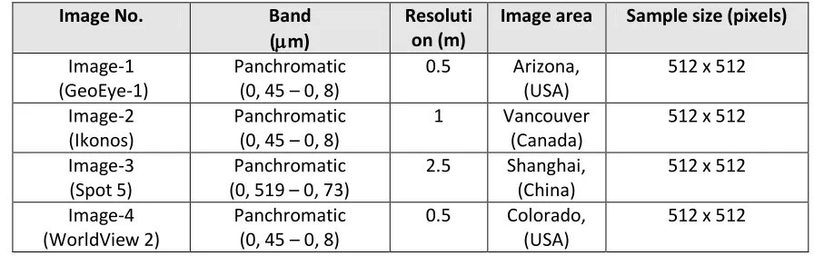
The data set used consists of four different types of images acquired by different satellites .Image-1 of GeoEye-1 satellite which is launched in September 2008. The satellite collects images at 0.5 meter panchromatic in the band (0.45 – 0.8) μm and 2 meter multispectral. Image-2 acquired by IKONOS satellite which collects panchromatic images with 1 meter resolution in the band (0.45 – 0.9) μm and multispectral imagery with 4 meter resolution at nadir. Image-3 acquired by spot5 satellite which has a 2.5 meter panchromatic in the band (0.519 – 0.73) μm resolution. Image-4 acquired by WorldView-2 satellite which is launched in October 2009 and considered the first high-resolution 8-band multispectral commercial satellite, operating at an altitude of 770 km. WorldView-2 provides images of 0.5 meter panchromatic in the band (0.45 – 0.8) μm and 2 meter multispectral *2+. +.Fig 1 shows the selected test set of image and Table (1) shows their characteristics.

A. B. C. D.

Image-1 (GeoEye-1) Image-2 (Ikonos) Image-3 (Spot 5) Image-4 (WorldView 2)

(3)

TABLE 1

Characteristics of test set images

Remote sensing Image Noise types and sources

Image noise is generally regarded as an undesirable by-product of image capture. The main sources of noise in remote sensing digital image can be [3, 4]:

a) The imaging sensor (photo detector) and the environmental conditions during image acquisition. b) Insufficient light levels and sensor temperature may introduce the noise in the image.

c) Interference in the transmission channel may also corrupt the image.

The most common types of noise in the remote sensing images are as following: Amplifier noise (Gaussian noise), Salt-and pepper noise, Shot noise (Poisson noise), and Speckle noise.

Amplifier noise (Gaussian noise)

The standard model of amplifier noise is additive, Gaussian, independent at each pixel and independent of the signal intensity, Amplifier noise is a major part of the "read noise" of an image sensor, that is, of the constant noise level in dark areas of the image, and it’s expressed mathematically as:

P(x) = 1/(σ√2π) *e(x-μ)2 / 2σ 2 -∞ < 0 <∞ (1)

Where:

P(x) is the Gaussian noise in image; μ and σ are the mean and standard deviation respectively.

Salt-and-pepper noise

An image containing salt-and-pepper noise will have dark pixels in bright regions and bright pixels in dark regions. This type of noise can be caused by dead pixels, analog-to-digital converter errors; bit errors in transmission, etc. [5] this can be eliminated in large part by using dark frame subtraction and by interpolating around dark/bright pixels. Salt & pepper distribution noise can be expressed by:

P1, x=A

P(x) = P2, x=B (2) 0, otherwise

Image No. Band

(m)

Resoluti on (m)

Image area Sample size (pixels)

Image-1 (GeoEye-1)

Panchromatic (0, 45 – 0, 8)

0.5 Arizona, (USA)

512 x 512

Image-2 (Ikonos)

1 Vancouver (Canada)

512 x 512

Image-3 (Spot 5)

2.5 Shanghai, (China)

512 x 512

Image-4 (WorldView 2)

0.5 Colorado, (USA)

(4)

Where:

p1, p2 are the Probabilities Density Function (PDF), p(x) is distribution salt and pepper noise in image and A, B are the arrays size image. Gaussian and salt & Pepper are called impulsive noise.

Poisson noise

Poisson noise or shot noise is a type of electronic noise that occurs when the finite number of particles that carry energy, such as electrons in an electronic circuit or photons in an optical device, is small enough to give rise to detectable statistical fluctuations in a measurement.

Speckle noise

Speckle noise is a granular noise that inherently exists in and degrades the quality of the active radar and synthetic aperture radar (SAR) images. Speckle noise in conventional radar results from random fluctuations in the return signal from an object that is no bigger than a single image-processing element. It increases the mean grey level of a local area. Speckle noise in SAR is generally more serious, causing difficulties for image interpretation. It is caused by coherent processing of backscattered signals from multiple distributed targets, it can be expressed by:

J = I + n*I (3) Where:

J is the distribution speckle noise image, I is the input image and n is the uniform noise image by mean o and variance v.

Concepts of Filters Used

Mean Filter:

The mean filter is a simple spatial filter .It is a sliding-window filter that replaces the centre value in the window. It replaces with the average mean of all the pixel values in the kernel or window. The window is usually square. The advantages of the mean filter are that Easy to implement and used to remove the impulse noise but its disadvantage that is it does not preserve details of image (Some details are removes of image with using the mean filter). [6]

Median Filter:

(5)

satisfactory in case of signal dependant noise. To remove these difficulties different variations of median filters have been developed for the better results. [6]

Wiener Filter:

The purpose of the Wiener filter is to filter out the noise that has corrupted a signal. This filter is based on a statistical approach. Mostly all the filters are designed for a desired frequency response. Wiener filter deals with the filtering of an image from a different view. The goal of wiener filter is to reduce the mean square error as much as possible. The Fourier domain of the Wiener filter is: [6]

(4)

Where:

H*(u, v) = Complex conjugate of degradation function Pn (u, v) = Power Spectral Density of Noise Ps (u, v) = Power Spectral Density of non-degraded image H (u, v) = Degradation function [6]

Bilateral filter

Recently most popular denoising method is the bilateral filter [7]. The bilateral filter is a nonlinear weighted averaging filter and also the weights depend on both the spatial distance and the intensity distance with respect to the centre pixel. The main feature of the bilateral filter is its ability to preserve edges while doing spatial smoothing. The bilateral filter is a robust filter because of its range weight, pixels with different intensities. It averages local small details and ignores outliers. At a particular pixel location n, the bilateral filter output is calculated as follows,

(5)

Where:

σd and σr are parameters controlling the fall-off of weights in spatial and intensity domains, respectively, N(x) is a spatial neighborhood of pixel I (x) , and C is the normalization constant[8]

(6)

Quality Assessment of the filtered images

The quality of the output filtered images is evaluated using the following five metrics:

Root mean square error (RMSE)

(6)

(7)

Where:

f(x,y)…….. The original or input image.

g(x,y)……. The output image (the filtered image). M x N …. The image size.

Peak signal to noise ratio (PSNR)

Peak signal to noise ratio is defined as [10, 11]:

]

))

,

(

)

,

(

1 log[

10

1 0 2 1 0 2 max



   





_N y M x

y

x

f

y

x

g

MxN

X

PSNR

[dB] (8)

Where, Xmax is the maximum gray level (255 for 8-bit level) of the given input image .The PSNR is more commonly used than the RMSE, because people tend to associate the quality of an image with a certain range of PSNR. Table 2 illustrates the PSNR values and its indication [9].

TABLE 2

The Peak Signal to Noise Ratio and its description

PSNR Description

Over 40 dB Excellent image (i.e., being very close to the original) )image).

Between 30 to 40 dB Good image (i.e., the distortion is visible but acceptable)

Between 20 and 30 dB Acceptable.

Lower than 20 dB Unacceptable.

Structural Similarity Index Measure (SSIM)

The conventional methods PSNR and MSE do not always agree with the subjective viewing results in case of additive distortion. The SSIM gives good evaluation accuracy and simple mathematical formulation.

It is based on comparing the structures of the reference and the filtered images. The structural information in an image can be defined as those attributes that represent the structure of objects in the scene, independent of the average luminance and contrast.

Structural Similarity (SSIM) index between signals x and y is,

SSIM x, y = *l(x, y)+α. *c x, y +β. *s x, y +γ (9) Where:

α > 0, β > 0 and γ > 0 are parameters used to adjust the relative importance of the three components. [11]



   







M 1

(7)

Discrepancy (D)

It is defined as:

(10) Where:

O i, j , F i, j are the pixel values at position (i, j) in the original images and the filtered images

respectively. M and N are the numbers or rows and columns of the image respectively. It is known that the spectral quality of the image increases as (D) decreases. [12]

Universal Image Quality Index (UIQI)

The UIQI is designed by modeling image distortion as a combination of three factors; loss of correlation, radiometric distortion, and contrast distortion. It is defined by the following formula:

(11)

Where:

σB_i∗Fi is the covariance between the band of filtered images and the input (original) images, μ and σ are

the mean and the standard deviation of the images. The dynamic range of UIQI is [-1, 1].The higher UIQI the better spectral quality image. [13]

Experimental Work & Results Evaluation

The filters were implemented using (MATLAB R2010b, 7.11.0) according to the following steps:

First, different types of noise are added to each one of the test original images to produce noisy images, tables (3-6) column 1,The Second, the four filters are used to filter the noisy image (The size of mean and median filters are a square window of size (3X3) ,Finally, comparing between resulting images depending on a quantitative measures: Peak Signal-to-Noise Ratio (PSNR), mean square error (MSE), (SSIM), (Discrepancy) and ( Universal Image Quality Index) metrics to determine the best proper filter in each case. Tables 3, 4, 5 and 6 show the results of applying the four filters on the images suffered from Poisson noise, Gaussian noise, speckle and salt & paper noises respectively. From these tables we have the following:

In case of Poisson Noise

The Bilateral filter gives the best results using (PSNR, MSE) metrics while by using the ( SSIM , Discrepancy and UIQI) metrics the Wiener filter gives more better results than the bilateral filter in images (1 and 4) with lightly difference.

In case of Gaussian noise

(8)

In case of Speckle noise

We found that the average filter gives the best results in images (1,2 and 4 ) using the five metrics while Wiener filter gives slightly good results more than the average filter in case of image (3) by using (MSE, PSNR and SSIM) metrics.

In case of Salt & Pepper noise

We found that approximately the median filter gives the best results in the four images using the five metrics.

Noisy images Average Median Wiener bilateral

(9)

TABLEIII

RESULTS FOR POISSON NOISE

Filter type Satellite images Resolution

[m]

Objective fidelity criterion

MSE PSNR SSIM D UIQI

Average

GeoEye-1 .5 132.0502 26.9234 0.9373 3.0816 0.9920

Ikonos 1 184.0873 25.4806 0.9497 3.7686 0.9790

Spot 5 2.5 312.3322 23.1846 0.9428 5.3750 0.9756

WV2 .5 71.5219 29.5864 0.9548 2.1860 0.9932

Median

GeoEye-1 .5 96.8387 28.2703 0.9341 2.6302 0.9941

Ikonos 1 153.5116 26.2694 0.9515 3.4662 0.9818

Spot 5 2.5 259.6449 23.9870 0.9538 4.7110 0.9791

WV2 .5 58.9664 30.4248 0.9497 2.0575 0.9939

Wiener

GeoEye-1 .5 50.0346 31.1381 0.9485 2.2373 0.9959

Ikonos 1 80.9107 29.0507 0.9686 2.6892 0.9892

Spot 5 2.5 167.7836 25.8833 0.9651 4.0924 0.9858

WV2 .5 33.5370 28.7994 0.9652 1.5925 0.9971

Bilateral

GeoEye-1 .5 46.6644 31.4409 0.9235 2.4863 0.9950

Ikonos 1 46.1169 31.4922 0.9710 3.0221 0.9907

Spot 5 2.5 54.7600 30.7462 0.9853 3.0997 0.9930

WV2 .5 33.2950 30.4496 0.9543 2.5392 0.9968

(10)

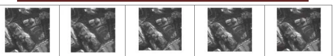
Fig (3) images contaminated by Gaussian noise (column 1) and the filtered images after applying the 4 filters

TABLEIV

RESULTS FOR GAUSSIAN NOISE

[m]

Average

GeoEye-1 .5 170.8049 25.8058 0.8777 3.7318 0.9879

Ikonos 1 222.1299 24.6647 0.9144 4.3775 0.9733

Spot 5 2.5 356.6540 22.6083 0.9236 5.7617 0.9729

WV2 .5 112.4676 27.6205 0.8477 3.2237 0.9912

Median

GeoEye-1 .5 161.5838 26.0468 0.8593 3.7230 0.9854

Ikonos 1 225.9253 24.5912 0.9045 4.5103 0.9721

Spot 5 2.5 348.3309 22.7109 0.9251 5.7022 0.9741

WV2 .5 126.9676 27.0939 0.8193 3.4601 0.9909

Wiener

GeoEye-1 .5 111.0649 27.6750 0.8849 3.2154 0.9888

Ikonos 1 149.4433 26.3860 0.9289 3.7154 0.9800

Spot 5 2.5 243.1387 24.2723 0.9431 4.8520 0.9810

WV2 .5 95.0214 28.3526 0.8448 3.0550 0.9929

Bilateral

GeoEye-1 .5 109.4437 27.7389 0.8389 4.7868 0.9598

Ikonos 1 128.5596 27.0398 0.9137 5.5824 0.9618

Spot 5 2.5 153.1960 26.2783 0.9566 5.5979 0.9782

(11)

Fig (4) images contaminated by Speckle noise (column 1) and the filtered images after applying the 4 filters

TABLEV

RESULTS FOR SPECKLE NOISE

[m]

Average

GeoEye-1 .5 286.7062 23.5564 0.7680 5.5021 0.9592

Ikonos 1 308.5672 23.2373 0.8580 5.6549 0.9482

Spot 5 2.5 423.7504 21.8597 0.9116 6.7764 0.9642

WV2 .5 139.9098 26.6723 0.8536 3.6196 0.9873

Median

GeoEye-1 .5 486.8936 21.2565 0.6926 7.6610 0.9183

Ikonos 1 464.6416 21.4596 0.8136 7.6951 0.9264

Spot 5 2.5 511.1086 21.0457 0.8956 8.4781 0.9544

WV2 .5 216.3898 24.7784 0.7751 4.7618 0.9803

Wiener

GeoEye-1 .5 293.7629 23.4508 0.7604 5.6596 0.9430

(12)

Spot 5 2.5 364.2405 22.5169 0.9270 6.2409 0.9643

WV2 .5 185.5247 25.4468 0.8501 3.8649 0.9770

Bilateral

GeoEye-1 .5 1100.0 17.7169 0.6908 11.502

6

0.8456

Ikonos 1 852.8286 18.8222 0.8238 9.7921 0.8973

Spot 5 2.5 662.3058 19.9202 0.9245 8.4211 0.9414

WV2 .5 379.5546 22.3381 0.8292 7.5892 0.9647

(13)

TABLEVI

RESULTS FOR SALT & PEPPER NOISE

[m]

Average

GeoEye-1 .5 196.6247 25.1944 0.8539 4.1480 0.9893

Ikonos 1 256.5437 24.0392 0.8944 4.5453 0.9712

Spot 5 2.5 397.0759 22.1421 0.9085 5.7088 0.9708

WV2 .5 141.1499 26.6340 0.8109 2.6570 0.9906

Median

GeoEye-1 .5 87.2534 28.7230 0.9656 1.8140 0.9956

Ikonos 1 146.9325 26.4596 0.9656 2.7519 0.9855

Spot 5 2.5 264.8416 23.9009 0.9543 4.1954 0.9797

WV2 .5 50.7917 31.0729 0.9753 1.4773 0.9948

Wiener

GeoEye-1 .5 300.5576 23.3515 0.8156 3.6646 0.9856

Ikonos 1 357.3606 22.5997 0.8780 4.0051 0.9736

Spot 5 2.5 444.4801 21.6523 0.9099 4.9280 0.9701

WV2 .5 363.0158 22.5315 0.7362 2.4808 0.9764

Bilateral

GeoEye-1 .5 302.5596 23.3227 0.7309 4.0925 0.9764

Ikonos 1 298.4476 23.3821 0.8427 3.6193 0.9772

Spot 5 2.5 330.2386 22.9425 0.9055 3.5773 0.9784

WV2 .5 294.9812 23.4329 0.6797 2.6958 0.9778

Conclusion

(14)

REFERENCES

1. Mrs. C. Mythili, Dr. V. Kavitha, “Efficient Technique for Color Image Noise Reduction”, IJJ The Research Bulletin of Jordan ACM 2011

2. Data sheets from http://www.digitalglobe.com, http://www.spotimage.com

3. Mr. Rohit Verma , Dr. Jahid Ali “A Comparative Study of Various Types of Image Noise and Efficient Noise Removal Techniques” International Journal of Advanced Research in Computer Science and Software Engineering, Volume 3, Issue 10, October 2013

4. Pawan Patidar, Manoj Gupta, Sumit Srivastava “Image De-noising by Various Filters for Different Noise” International Journal of Computer Applications (0975 – 8887)Volume 9– No.4, November 2010

5. Mr. Salem Saleh Al-amri, Dr. N.V. Kalyankar and Dr. Khamitkar S.D “ A Comparative Study of Removal Noise from Remote Sensing Image” IJCSI International Journal of Computer Science Issues, Vol. 7, Issue. 1, No. 1, January 2010

6. Priyanka Kamboj, Versha Rani “A BRIEF STUDY OF VARIOUS NOISE MODEL AND FILTERING TECHNIQUES” Journal of Global Research in Computer Science, 4 (4), April 2013.

7. M.Vijay, L.Saranya Devi “Speckle Noise Reduction in Satellite Images Using Spatially Adaptive Wavelet Thresholding” International Journal of Computer Science and Information Technologies, Vol. 3 (2) , 2012

8. Ming Zhang “BILATERAL FILTER IN IMAGE PROCESSING” Department of Electrical and Computer Engineering Beijing University of Posts and Telecommunications August 2009

9. AL Bovik, "Hand book of Image and Video Processing", Department of Electrical and Computer Engineering, The University of Texas at Austin, 2000

10. Guy E.Blelloch ,"Introduction to Data Compression ",Guy E.Blelloch, computer science department, Carnegie Mellon University, October 16,2001.

11. Shruti Sonawane and A. M. Desh pande “Image Quality Assessment Techniques: An Overview” International Journal of Engineering Research & Technology (IJERT) Vol. 3 Issue 4, April – 2014 12. M. Fallah Yakhdani , A. Azizi “Quality Assesment of Image Fusion Techniques for Multi sensor High

Resolution Satellite Images “.ISPRS TC VII Symposium July 5–7, 2010.