Direct Simulation of Quantum Dynamics in Complex Systems

(1)

Direct Simulation of Quantum Dynamics

in Complex Systems

Thesis by

Artur R. Menzeleev

In Partial Fulfillment of the Requirements for the Degree of

Doctor of Philosophy

California Institute of Technology Pasadena, California

2014

(2)

c 2014

(3)

(4)

Acknowledgments

First, I would like to thank Dr. Thomas F. Miller, my advisor. Over the course of my graduate work, he has taught me much about being a scientist, as well as the value of imagination, tenacity, rigor, and hard work.

I would also like to thank the faculty of the Division of Chemistry and Chemical Engineering. In particularly, I would like to thank my thesis committee, Dr. Rudy Marcus, Dr. Harry Gray, and Dr. Mitchio Okumura for continuing support and valuable scientific discussions. Also, I remember Dr. Aron Kuppermann, his inspirational presentation of the intricacies of quantum mechanics, and his friendly conversations.

I appreciate the support of division administrative and technical staff, in particular Priscilla Boon, who is instrumental to the smooth running of the chemical physics subdivision and the Miller Group. Also, I thank Agnes Tong, Anne Penney, and Tom Dunn for their technical and administrative expertise. Finally, I am thankful for the technical aid of the Caltech High-Performance Computing staff, in particular Zailo Leite and Naveed Near-Ansari.

I greatly appreciate the friendly and supportive demeanor of the Miller Group. Bin, Nick, Nandini, Jason, Josh, Connie, Taylor, Mike, Fran, Kuba, Frank, Romelia, Michiel, Joonho, and Matt—thank you all for the scientific discussion over the years, the feedback on my ideas, and the great company. Thank you also to my friends both outside the lab and outside of Caltech.

(5)

Abstract

Accurate simulation of quantum dynamics in complex systems poses a fundamental theoretical challenge with immediate application to problems in biological catalysis, charge transfer, and solar-energy conversion. The varied length- and timescales that characterize these kinds of processes ne-cessitate development of novel simulation methodology that can both accurately evolve the coupled quantum and classical degrees of freedom and also be easily applicable to large, complex systems. In the following dissertation, the problems of quantum dynamics in complex systems are explored through direct simulation using path-integral methods as well as application of state-of-the-art an-alytical rate theories.

Chapter 1 describes the investigation of the distance dependence of rates of long-range proton-coupled electron transfer (PCET) reactions. In concert with experimental observations, we employ molecular dynamics and electronic structure methods, applied within the framework of analytical rate theories, to determine, for the first time, the redox donor-acceptor distance decay constant,

β, associated with a concerted proton-coupled electron transfer (CPET) reaction. We show that, although the calculation ofβ is sensitive to specific details of the theoretical assumptions, values of

β obtained from studies of electron transfer (ET) reactions can be directly applied to vibronically nonadiabatic CPET reactions. The collaborative study is published as Warren, J. J., Menzeleev, A. R., et al., “Long-range proton-coupled electron-transfer reactions of bis(imidazole) iron tetraphenyl-porphyrins linked to benzoates,”Journal of Physical Chemistry Letters,4, 519 (2013).

(6)

beyond the linear response regime: excess electron injection and trapping in liquids,” Journal of Chemical Physics,132, 034106 (2010).

Chapter 3 explores the use of RPMD to directly simulate ET reactions between mixed-valence transition metal ions in water. We compare the RPMD approach against benchmark semiclassical and quantum dynamics methods in both atomistic and system-bath representations for ET in a polar solvent. Without invoking any prior mechanistic or transition state assumptions, RPMD correctly predicts the ET reaction mechanism and quantitatively describes the ET reaction rate over twelve orders of magnitude in the normal and activationless regimes of ET. Detailed analysis of the dynamical trajectories reveals that the accuracy of the method lies in its exact description of statistical fluctuations, with regard to both reorganization of classical nuclear degrees of freedom and the electron tunneling event. The vast majority of the ET reactions in biological and synthetic systems occur in the normal and activationless regimes, and this work provides the foundation for future studies of ET and PCET reactions in condensed-phase systems. Additionally, this study discovers a shortcoming of the method in the inverted regime of the ET, which arises from the inadequate description of the quantization of the real-time electronic-state dynamics, and directly motivates further methodological refinement. This work has been published as Menzeleev, A. R., Ananth, N. and Miller, T. F., “Direct simulation of electron transfer using ring polymer molecular dynamics: Comparison with semiclassical instanton theory and exact quantum methods,”Journal of Chemical Physics,135, 074106 (2011).

(7)

List of Figures

1.1 Thermochemical cycle for PCET reactions . . . 2

1.2 RPCET Reaction ofFeIIIPhnCO – 2with TEMPOH . . . 3

1.3 The system employed in MD calculation ofw(_rn)(R) . . . 10

1.4 Free energy profilesw(_rn)(R) andw_p(n)(R) . . . 14

1.5 Outer-sphere CPET reorganization energies computed using MD . . . 18

1.6 Outer-sphere CPET reorganization energies computed using FRCM . . . 19

1.7 Distributions of the proton donor-acceptor distances in iron-porphyrin-TEMPOH com-plexes . . . 21

1.8 Atom types for then= 1 iron-porphyrin complex. . . 25

1.9 Atom types for then= 2 iron-porphyrin complex. . . 28

1.10 Atom types for the TEMPOH molecule. . . 31

2.1 Cold electron injection into supercritical helium . . . 64

2.2 Ring polymer radius of gyration following injection . . . 65

2.3 Hot electron injection into supercritical helium . . . 66

2.4 Time-resolved radial distribution functionhge−He(r, t)i . . . 68

2.5 Eigenstates of the excess electron following electron injection into supercritical helium 69 2.6 Time-resolved radial distribution function hge−He(r, t)i for simulations with 4096 He atoms . . . 70

2.7 Components of the system energy following cold electron injection into helium . . . . 71

2.8 Components of the system energy following hot electron injection into helium . . . 72

2.9 Energy dissipation following electron injection into helium . . . 73

2.10 Ring polymer radius of gyration following excess electron injection into liquid water . 75 2.11 Solvent dynamics following cold electron injection into water . . . 76

2.12 Solvent dynamics following hot electron injection into water. . . 77

2.13 Excess electron eigenstates following electron injection into water . . . 77

(12)

3.1 Snapshots of the atomistic representation of the ET reaction . . . 98

3.2 Free energy profiles for the ET reaction in the atomistic representation . . . 111

3.3 ET reaction rates and representative trajectories in the atomistic representation – nor-mal and activationless regimes . . . 113

3.4 ET reaction rates and representative trajectories in the atomistic representation – in-verted regime . . . 115

3.5 ET reaction rates and FE profiles for Model SB1 . . . 116

3.6 Comparison of ET rates for Marcus-like and “direct” mechanisms . . . 118

3.7 NormalizedCFF(t) for ET reaction in Model SB2 . . . 119

4.1 A schematic illustration of ring-polymer configurations that exhibit kink-pairs. . . . 136

4.2 Thermal reaction rate coefficients for System A . . . 151

4.3 ET reaction rate coefficients for System B in classical and quantized solvent . . . 153

4.4 Representative trajectories from the ensemble of reactive KC-RPMD trajectories in various regimes of ET . . . 154

(13)

List of Tables

1.1 Values of electronic decay constantβ. . . 23

1.2 Atom types and charges in the reactant and product states for then= 1 iron porphyrin complex. . . 26

1.3 Atom types and charges in the reactant and product states for then= 2 iron porphyrin complex. . . 29

1.4 TEMPOH atom types and charges in the reactant and product states. . . 31

1.5 Optimized Cartesian coordinates of the TEMPO molecule . . . 32

1.6 Optimized Cartesian coordinates of the TEMPOH molecule . . . 33

1.7 Optimized Cartesian coordinates of theFeIIIPhCO–₂molecule . . . 34

1.8 Optimized Cartesian Coordinates of theFeIIPhCO₂H molecule . . . 37

1.9 Optimized Cartesian Coordinates of theFeIIIPh₂CO–₂ molecule . . . 40

1.10 Optimized Cartesian Coordinates of theFeIIPh₂CO₂Hmolecule . . . 43

1.11 Energies for the optimized geometries provided in Tables 1.7-1.10 . . . 45

1.12 Cartesian coordinates of the rigid portion of the iron-porphyrin speciesFeIIIPhCO–₂ employed in calculation ofw(1)_r (R) andw(2)_r (R) . . . 46

1.13 Cartesian coordinates of the rigid portion of the iron-porphyrin speciesFeIIIPh₂CO–₂ employed in calculation ofw(1)_r (R) andw(2)_r (R) . . . 48

1.14 Cartesian coordinates of the rigid portion of the iron-porphyrin speciesFeIIPhCO₂H employed in calculation ofw(1)_p (R) andw(2)_p (R) . . . 50

1.15 Cartesian coordinates of the rigid portion of the iron-porphyrin speciesFeIIPh₂CO₂H employed in calculation ofw(1)p (R) andw(2)p (R) . . . 52

3.1 Complex timestk used to calculate the {Bkk0}. . . 97

3.2 Parameters for the atomistic representation of ET. . . 99

3.3 Values of the asymmetry parameterconsidered in the atomistic representation . . . 100

3.4 Values of the asymmetry parameterconsidered in the system-bath representation . . 102

(14)

3.6 ET reaction rates for the atomistic representation, obtained using RPMD and Marcus

theory. . . 110

3.7 ET reaction rates for Model SB1, obtained using RPMD, Marcus theory, and SCI theory115 3.8 ET reaction rates for a 1D asymmetric double well, obtained using SCI theory. . . . 117

3.9 ET reaction rates for Model SB2, obtained using RPMD, Marcus theory, SCI theory, and exact quantum dynamics . . . 119

3.10 Parameters for the left Coulombic well in Model SB1 . . . 121

3.11 Parameters for the right Coulombic well in Model SB1 . . . 121

3.12 Parameters for the left Coulombic well in Model SB2 . . . 122

3.13 Parameters for the right Coulombic well in Model SB2 . . . 122

3.14 The diagonal elements of the diabatic potential matrix for Model SB2. . . 124

4.1 Parameters for System A. . . 144

4.2 Values ofmy for the KC-RPMD simulations of System A. . . 144

(15)

Chapter 1

Theoretical aspects of investigating distance dependence of

CPET reactions of bis(imidazole) iron tetraphenylporphyrins

1.1

Introduction

Electron transfer (ET) reactions coupled to proton transfer(PT) reactions are common in chemistry in biology. This process can occur sequentially, with ET followed by PT, PT followed by ET, or in a concerted fashion, where the electron and proton transfer in a single chemical step. The latter process, CPET, is implicated in biological processes that involve spatial separation of the donor and acceptor sites.1–3 The oxidation of tyrosine Z in photosystem II, for example, is a prototypical separated CPET reaction, with PT occurring between the tyrosine and a nearby histidine and ET occurring between tyrosine and oxidized chlorophyll P680+located nearly 10 ˚A away.1

(16)

1.2

Summary of thermochemical and kinetic properties of

the model PCET reactions

This study is concerned with PCET reactions of iron complexes of 5-(4-carboxyphenyl)-10,15-20-triphenyl-porphyrin (FeIIIPhCO₂H) and 5-(1,10-biphenyl-4-carboxylic acid)-10,15,20-triphenylpor-phyrin (FeIIIPh₂CO₂H), which differ by the number of phenylene spacers between the heme and the acid moiety. These compounds were synthesized and metalated according to published proce-dures.8–10Spectroscopic and electrochemical evidence indicate that the heme-iron and the benzoate moiety of these compounds are largely electronically uncoupled, and that the thermochemical prop-erties of the iron systems are in general very similar.7The thermochemical properties of the PCET reactions are given in Figure 1.1.

Figure 1.1: Thermochemical cycle relevant to PCET reactions of bis(imidazole) iron tetraphenyl-porphyrins linked to benzoates

The deprotonated ferric compounds FeIIIPhCO–₂ and FeIIIPh₂CO–₂, reacted with 2,20-4,40 -tetramethylpi-peridin-1-ol (TEMPOH) to yield the ferrous speciesFeIIPhCO₂HandFeIIPh₂CO₂H

(Figure 1.2). The reaction rates under pseudo-first-order condition of excess TEMPOH at 298K were determined to be: k(1) = 15.3±1.4M−1s−1 andk(2) = 6.5±0.8M−1s−1. The KIE was not deter-mined due to a competing precipitation reaction, however, the initial rates were clearly slower for the transfer of deuterium.

(17)

Figure 1.2: PCET Reaction ofFeIIIPhnCO –

2with TEMPOH

TEMPOH strongly favors CPET in order to avoid high-energy intermediates that would be generated by individual ET or PT reactions. Specifically, for the CPET from TEMPOH toFeIIIPhCO–₂, the driving force is ∆GoCPET = −3.5±1.1 kcal/mol, whereas the driving forces for the PT and ET

reactions are ∆Go_PT = 28.5 kcal/mol and ∆Go_ET = 29.6 kcal/mol, respectively. The measured barrier ∆G‡ = 15.8 kcal/mol is below the ∆Go_PT and ∆Go_ET, which indicates that the reaction occurs by a CPET mechanism. The PCET reaction between FeIIIPh₂CO–₂ and TEMPOH has ∆Go_CPET =−3.7±1.1 kcal/mol, ∆G_PTo = 28.2 kcal/mol, ∆Go_ET= 29.4 kcal/mol, and ∆G‡ = 16.3 kcal/mol and therefore also occurs by CPET.

The observed twofold decrease in measured bimolecular PCET rate is consistent with previous unimolecular observations of ET through phenylene linkers.4 However, the determination of the electronic coupling constantβ from the measured reaction rates involves factors that are difficult to obtain experimentally. The following sections describe the theoretical formulation and calculations that were performed to obtain the value ofβ.

1.3

Theoretical analysis

1.3.1

A simplified bimolecular CPET rate expression

In this section, a simplified rate equation is derived for the CPET between FeIIIPhnCO – 2 and TEMPOH. The full equation for the bimolecular, vibronically non-adiabatic CPET is11–13

k=

Z dR

Z drX

j

X

k 2π

~

Pj|Vjk|2(4π(λ+ ∆λjk)kBT)− 1

2 (1.1)

×exp

−β(∆G

o₊_λ_{+ ∆}_λ

jk+k−j)2 4(λ+ ∆λjk)

exp[−βwr].

(18)

(19)

(20)

for r and R are statistically uncorrelated for configurations that contribute to the CPET rate, it follows that the joint probability distribution factorizes,

ρ(r, R) =ρ(r)ρ(R), (1.8)

such that the potential of mean force associated with these coordinates is additive,

wr(r, R) =wr(R) +wr(r). (1.9)

A similar argument holds for the preorganization work for the products,wp(r, R).

The driving force ,∆Go(r, R), for the CPET reaction at a particular value ofr and R is given by15–17

∆Go(r, R) = ∆Go_CPET+wp(r, R)−wr(r, R), (1.10)

where ∆Go_CPETis the driving force at infinite separation with respect to eitherrorR. The preceding analysis ofwr(r, R) andwp(r, R) thus leads to an additive expression for the driving force,

∆Go(r, R) = ∆Go(r) + ∆Go(R). (1.11)

Lastly, note that in the regime of weak electronic coupling (HAB kBT ), the CPET vibronic

coupling takes the form4–6

Vjk(r, R) =hj|HAB(r, R)|ki, (1.12)

where HAB(r, R) is the electronic coupling matrix element, and |ji and |ki are the reactant and

product vibrational wavefunctions, respectively. We then employ the standard Condon approxima-tion that the electronic coupling is insensitive to changes in the proton posiapproxima-tion over the lengthscale of the proton vibrational wavefunctions, such thatHAB(r, R) =HAB(R) , and18–20

Vjk(r, R) =HAB(R)hj|ki(r). (1.13)

(21)

(22)

λ(R). These terms are calculated using a mixture of molecular dynamics and electronic structure techniques, which are described in detail in this section. The computational model employed is presented in Section 1.4.1. The subsequent sections describe the calculation of the individual terms appearing in the CPET rate equation: Section 1.4.2 describes the calculation of the preorganization work terms, Section 1.4.3 describes the calculation of the inner- and outer-sphere reorganization energies, and Section 1.4.4 describes the calculation of the driving forces. The force field parameters of the computational model and optimized molecular geometries are presented in Appendices A and B to this chapter.

1.4.1

Description of the MD simulations

MD simulations of the PCET reactants employ a system comprised ofFeIIIPhCO–₂,FeIIIPh₂CO–₂, and a single TEMPOH molecule; simulations of the products employ a system comprised of

FeIIPhCO₂H, FeIIPh₂CO₂H, and a single TEMPO molecule. In both cases, the system also includes 2225 acetonitrile molecules. The simulation is performed in a 46.8 ˚A× 91.2 ˚A× 46.8 ˚A rectangular unit cell that is subject to periodic boundary conditions.

The porphyrin molecules, axial ligands, and TEMPOH/TEMPO molecules are modeled using the Generalized Amber Force Field (GAFF),21which is implemented within the DLPOLY molecular dynamics package.22The iron atom in both oxidation states is modeled using the Giammona param-eters, which are included as the frcmod.hemall contributed parameter set for AMBER.23Atom-type assignment (Tables 1.2-1.4) is performed using the Antechamber program.24 Acetonitrile molecules are represented with the three-site model of Guardia et al.,25 in which the methyl group is repre-sented as a single particle. In all calculations, the N-methylimidazole axial ligands are replaced by imidazole ligands.

In all MD simulations, short-range interactions are truncated atrcut= 12˚A, and force-shifting26

is employed for the truncation of long-range electrostatic interactions. Trajectories are thermostatted at a temperature of 298 K by resampling all atomic velocities from the Boltzmann distribution every 50 ps, and a timestep of 0.25 fs is employed to ensure accurate integration of the bond-stretching modes.

(23)

equation formalism of the polarizable continuum model,28,29with the default parameter values of the implementation in Gaussian 09.30 The solute cavity is assembled from atom-centered spheres with radii corresponding to the atomic radii in the Universal Force Field (UFF) scaled by 1.1. The cavity surface is smoothly represented using the GePol-YK scheme,31and the acetonitrile static and optical dielectric constants have values ofo= 35.688 and∞= 1.806874, respectively. Atomic point charges

(Tables 1.2-1.4) are determined by fitting the electrostatic potential from the electronic structure calculations using CHelpG (CHarges from Electrostatic Potentials using a Grid based method);32 the charges for all atoms of the same atom-type are set to the mean value obtained from the CHelpG calculation.

In all MD simulations, the TEMPOH and TEMPO molecules are kept rigid at geometries that are optimized at the B3LYP/6-31G(d,p) level of theory; both molecules are most stable in the chair conformation with the oxygen atom in the equatorial position, and the OH torsion in TEMPOH assumes the anti conformation with respect to the axial methyl groups. The metalated porphyrin ring, the meso substituents, and the axial ligands are also held rigid at the optimal geometry ob-tained at the B3LYP/6-31G(d,p) level, while the phenylene linker regions are left unrestrained. The NOSQUISH algorithm33is employed to integrate the rigid-body equations of motion in the MD simu-lations. The optimized molecular geometries of TEMPO, TEMPOH,FeIIIPhCO–₂,FeIIPhCO₂H,

FeIIIPh₂CO–₂, and FeIIPh₂CO₂H, are included in Tables 1.2-1.4.

1.4.2

Calculation of

w

_r(n)

(

R

)

and

w

_p(n)

(

R

)

This section describes the MD simulations that are used to calculate the reactant and product free energy profiles as a function of the electron donor-acceptor distance, w_r(n)(R) and w(_pn)(R), respectively. To robustly and efficiently obtain the relative free-energy profiles for the shorter (n= 1) phenylene linker relative to the corresponding profiles for the longer (n= 2) linker, some care must be taken in the design of the simulation protocol, as is now described.

(24)

Figure 1.3: The system employed in molecular dynamics calculation ofw_r(n)(R). Fixed regions of the porphyrin molecules are indicated in gray, the flexible linker region ofFeIIIPhCO–₂is indicated in red, and the flexible linker region of FeIIIPh₂CO–₂ is indicated in blue. The rigid TEMPOH molecule is yellow, and the TEMPOH oxygen atom is indicated in purple. The porphyrin 5-carbon atoms defining the R(1) and R(2) distances (see text) are indicated with gray spheres, and the carboxylic carbons defining the ξ(1) and ξ(2) distances are indicated with orange spheres. MeCN molecules are omitted for clarity. The region of the application of cylindrical restraint Vcyl(d) is

indicated with gray dashed-dot lines.

(detailed geometries provided in Tables 1.14 and 1.15).

To compute the reactant free energy profiles, we begin by defining collective variables associated with the electron donor-acceptor distance for the n = 1 and n = 2 complexes in the simulation setup. Specifically,R(1)andR(2)denote the Euclidean distance between the TEMPOH oxygen and the 5-carbon of the porphyrin ring ofFeIIIPhCO–₂ orFeIIIPh₂CO–₂, respectively (Fig. 1.3). We then define ∆R = R(1) −R(2) and R = min(R(1), R(2)) in terms of these simple donor-acceptor distances. It is clear that any atomistic configuration for the system corresponds to a particular value for the collective variables ∆R and R. Furthermore, it is clear that the collective variables distinguish between configurations for which the system occupies the basin of stability for then= 1 complex (smallR, negative ∆R), for which the system occupies the basin of stability for the n= 2 complex (smallR, positive ∆R), and for which the system is transferring between these two basins of stability (largerR, ∆R≈0).

By sampling the full probability distribution in these two coordinates,Pr(∆R, R), we have a direct

means of comparing the relative free energies of these two basins of stability (i.e., the difference of the reversible work of association for the n= 1 and n = 2 TEMPOH-FeIIIPh_nCO–₂ complexes). Specifically, this relative free energy can be evaluated using

−kBTln

Z c −∞

d∆R Z ∞

0

dRPr(∆R, R) +kBTln

Z ∞

c

d∆R Z ∞

0

(25)

(26)

(27)

andS(rOH) is the sigmoid function

S(rOH) = 0.5 (1 + erf (2.0 (−rOH+ 3.0))). (1.27)

Here, φis the dihedral angle formed by the TC1, TN, and OC atoms of the TEMPO molecule and the HT atom of the nearest carboxylic acid, and rOH is the distance between the OC atom and

the HT atom. This restraint thus applies when TEMPO is hydrogen-bound to the carboxylic acid moiety ofFeIIPhCO₂Hor FeIIPh₂CO₂H, and it does not bias the simulation when TEMPO is free in solution. We use parameters ∆φ= 1.5 rad, φ0= 1.5 rad, andkφ= 3.0 kcal/mol/rad2.

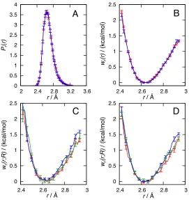
Figure 1.4A presents the free energy surface associated with the reduced two-dimensional prob-ability distribution for the reactant species, −kBTlnPr(∆ξ, R) (see Eqs. 1.22 and 1.23). The free

energy surface is characterized by two pronounced basins of stability; the basin at (∆ξ ≈ −20˚A,

R ≈ 8˚A) corresponds to the n = 1 complex in which TEMPOH is bound to the FeIIIPhCO–₂

molecule, and the basin at (∆ξ ≈ 20˚A, R ≈ 12˚A) corresponds to the n = 2 complex in which TEMPOH is bound to the FeIIIPh₂CO–₂molecule. The intermediate, featureless region for which −20˚A < ∆ξ < 20˚A corresponds to configurations for which the TEMPOH is not directly bound

to either iron-porphyrin molecule. Figure 1.4B presents the free energy surface associated with the reduced two-dimensional probability distribution for the product species,−kBTlnPp(∆ξ, R), which

also shows basins associated with then= 1 andn= 2 complexes.

(28)

TEM-Figure 1.4: Free energy surfaces obtained using MD simulations. (A) The two-dimensional reac-tant free energy surface,−kBTlnPr(∆ξ, R). (B)The two-dimensional product free energy surface,

−kBTlnPp(∆ξ, R). In panels A and B, the contour lines denote increments of 1 kcal/mol. (C)The

reactant free energy profiles,wr(n)(R), for the n= 1 (red) andn= 2 (blue) complexes as a function

of the electron donor-acceptor distance. (D) The product free energy profiles, wp(n)(R), for the

n= 1 (red) and n= 2 (blue) complexes as a function of the electron donor-acceptor distance. The structures in panel D illustrate configurations of the TEMPO associated with different orientations of the carboxylic acid OH bond.

POH andFeIIIPhnCO –

2molecules.

(29)

are due to the torsional potential associated with rotation of the carboxylic acid OH bond, which exhibits local minima in configurations for which the acidic proton lies in the plane of the other of carboxylate atoms. As a result of this torsional potential, the acidic proton can either point away from the linker into solution, or it can point back towards the linker. The TEMPO molecule, which forms a hydrogen bond with the acidic proton, thus adopts two orientations that are characterized by differing values of the electron donor-acceptor distances. We illustrate these orientations in the inset of Figure 1.4D.

1.4.3

Calculation of the CPET reorganization energies

1.4.3.1 Calculation of λi

The inner-sphere CPET reorganization energies, λ(_in), are computed as the sum of individual con-tributions from the iron-porphyrin complex and TEMPOH,36,37

λ_i(n)=λ(_i_,n_FePor) +λi,TEMPOH (1.28)

The inner-sphere reorganization of the iron-porphyrin complex is calculated using38,39

λ(_i_,n_FePor) =E FeIIPh_nCO₂H|FeIIIPh_nCO−₂

−E FeIIPh_nCO₂H|FeIIPh_nCO₂H

, (1.29)

where E(A|B)denotes the energy of species A at the optimized geometry of species B. (In the calculation of E FeIIPhnCO2H|Fe

III

PhnCO−2

, the position of the additional proton is optimized while keeping all other atoms fixed.) The corresponding term for TEMPOH is calculated using

λi,TEMPOH=E(TEMPO|TEMPOH)−E(TEMPO|TEMPO). (1.30)

By treating these contributions separately, we make the usual assumption that the inner-sphere reorganization energies are unaffected by preorganization of the CPET donor and acceptor species. In all cases, the geometry optimizations are performed at the B3LYP/6-31G(d,p) level of theory, with solvation effects included via the polarizable continuum model using the default parameters for Gaussian 09 (version G09RevB.01); final energies are computed using B3LYP/TZVP without implicit solvent effects.

These calculations yield λi,TEMPOH = 16.74 kcal/mol, λ (1)

i,FePor = 8.21 kcal/mol, and λ (2) i,FePor =

(30)

the structural rearrangement of the acid moiety upon protonation, with the rearrangements in the porphyrin ring and its substituents contributing only approximately 1 kcal/mol; this is confirmed by repeating the calculation of E FeIIPh_nCO₂H|FeIII_Ph

nCO

−

2

while fixing the position of atoms other than the carboxylic acid moiety. The small inner-sphere reorganization energy for the por-phyrin obtained here is consistent with previous studies of model heme compounds, where the total inner-sphere reorganization energy in a self-exchange ET reaction between FeIII(porphine)(Im)₂and FeII(porphine)(Im)–₂ was shown to be only 1.95 kcal/mol.40 Similarly, the insensitivity of λ(_i_,n_FePor)

to number of phenylene linkers is consistent with earlier computational studies of unmetalated N-methylmesoporphyrin, in which the structure of the porphyrin macrocycle was shown to be largely independent of the side chains decorating the ring.41

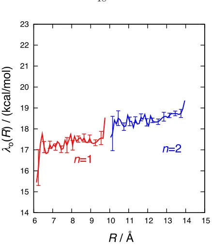
1.4.3.2 Calculation of λo(R) using all-atom MD simulations

The outer-sphere CPET reorganization energy,λ(_on)(R), is calculated using the MD simulation model described in Sections 1.4.1 and 1.4.2. For a given electron donor-acceptor distanceR, the reorgani-zation energy is obtained using42–44

λ(_on)(R) =1 2

h∆U(n)ir(R)− h∆U(n)ip(R)

, (1.31)

where

h∆U(n)iµ(R) =Z_R−1 Z

dxe−

Uµ(x)

k_BT _δ₍_R₍_x₎₋_R_{) ∆}_U(n)₍_x₎_, _(1.32)

ZR=

Z dxe−

Uµ(x)

kBT _δ₍_R₍_x₎₋_R₎_, _(1.33)

and

∆U(n)(x) =U_p(n)(x)−U_r(n)(x). (1.34)

Here, x denotes the configuration of the solute and solvent, Uµ(x) is the total potential energy function for the system in the reactant (µ = r) or product (µ = p) state, and U_µ(n)(x) denotes the subset of pairwise interactions between the acetonitrile solvent and the solute complex with n

(31)

outer-sphere reorganization energy without resolving the dependence onR using

λ(_on)= 1 2

h∆U(n)ir− h∆U(n)ip

, (1.35)

and

h∆U(n)iµ=Z−1 Z

dxe−

Uµ(x)

kBT _∆_U(n)₍_x₎_. _(1.36)

In the calculation of ∆U(n)(x), the energy functions are evaluated at reactant and product ge-ometries that are identical, except for the position of the transferring proton (HT). In the calculation ofh∆U(n)ir(R), the position of HT in the product state (needed for the Up(n)(x) term) is obtained

via reflection of its position in the reactant state through the plane that perpendicularly bisects the segment between the TEMPOH oxygen (OC, the proton donor) and the acidic carboxylate oxygen (OA, the proton acceptor). For the calculation ofh∆U(n)ip(R), the reverse operation is performed

to obtain the position of HT in the reactant state.

For the calculation of λ(1)_o (R), the equilibrium ensemble for the reactant state is sampled using 1200 uncorrelated snapshots from an unrestrained, 6 ns NVT simulation of the system in the basin of stability for which TEMPOH is hydrogen-bonded toFeIIIPhCO–₂; the equilibrium ensemble for the product state is sampled using 1000 uncorrelated snapshots from an unrestrained, 5 ns NVT simulation of the system in the basin of stability for which TEMPO occupying is hydrogen-bonded toFeIIPhCO₂H. Similarly, for the calculation ofλ(2)_o (R), the equilibrium ensemble for the reactant state is sampled using 1500 uncorrelated snapshots from an unrestrained, 7.5 ns NVT simulation of the TEMPOH-FeIIIPh₂CO–₂ complex; the equilibrium ensemble for the product state is sampled using 1000 uncorrelated snapshots from an unrestrained, 5 ns NVT simulation of the

TEMPO-FeIIPh₂CO₂Hcomplex.

Figure 1.5 presents the computed CPET outer-sphere reorganization energiesλ(1)_o (R) andλ(2)_o (R) as a function of the electron donor-acceptor distance. For a given number of phenylene linkers, the reorganization energy depends only weakly onR. It is also weakly sensitive to the number of linkers,

(32)

(33)

˚

A). The optical and static dielectric constants employed for the acetonitrile solvent are 0 = 37.5

and ∞= 1.79, respectively. The FRCM calculations are performed using the webPCET software

package.47

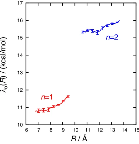
For the calculation of λ(1)_o (R), the solute configurations are obtained by taking 4000 uncorre-lated configurations from an unrestrained, 8 ns simulation of the TEMPOH-FeIIIPhCO–₂complex. Similarly, for λ(2)_o (R) complex, the solute configurations are obtained by taking 3000 uncorrelated configurations from an unrestrained, 6 ns simulation of the TEMPOH-FeIIIPh₂CO–₂complex. For each configuration, the reactant and product geometries are identical, except that the position of the transferring proton (HT), which is obtained as in Section 1.4.3.2. The charge distributions for the reactant and product state of both complexes are described in Appendix A.

10 11 12 13 14 15 16 17

6 7 8 9 10 11 12 13 14 15

R

/ Å

!

λ

o

(

R

)

/

(kca

l/

mo

l)

!

n

=1

!

n

=2

!

Figure 1.6: Outer-sphere CPET reorganization energies, λon(R), for the complexes with n = 1 (red) andn= 2 (blue) phenylene linkers, computing using the FRCM.

(34)

1.4.4

Calculation of

∆

G

o(n)

and

∆∆

G

o

.

In this section, we validate the assumption that ∆Go is small in comparison to λ for the CPET reactions considered in this study, and we calculate the difference in the reaction driving forces at infinite separation, ∆∆Go.

For each complex, the driving force at infinite separation is calculated using

∆Go_CPET(n) =E(FeIIPh_nCO₂H) +E(TEMPO)−E(FeIIIPh_nCO−₂)−E(TEMPOH), (1.39)

whereE(A) represents the energy of species A. As before, geometry optimizations are performed at the B3LYP/6-31G(d,p) level of theory, with solvation effects included via the polarizable continuum model using the default parameters for Gaussian 09 (version G09RevB.01); final energies are com-puted using B3LYP/TZVP with implicit solvent effects included. We compute ∆Go_CPET(1) =−3.43 kcal/mol, and ∆Go_CPET(1) =−3.69 kcal/mol, which are in agreement with the experimental estimates of ∆Go_CPET(1) = −3.5±1.1 kcal/mol and ∆G_CPETo(2) = −3.7±1.3 kcal/mol. The values for ∆Go at finite separations, obtained using Eq. 1.10 and the results in Figs. 1.4C and 1.4D, are comparable or smaller in magnitude than the corresponding values for ∆Go at infinite separations.

The difference in the reaction driving forces at infinite separation is calculated as

∆∆Go= ∆Go_CPET(1) −∆Go_CPET(2) (1.40)

Using the driving force values described above, we obtain ∆∆Go= 0.26 kcal/mol, which is again in agreement with the experimentally measured value of ∆∆Go= 0.2±1.4 kcal/mol.

1.4.5

Decorrelation of the proton and electron donor-acceptor distances,

and insensitivity of the proton donor-acceptor distance distribution

to phenylene linker length.

Various simplifications in the derivation of the CPET rate expression (Section 1.3) follow from the assumption that the proton donor-acceptor distance, r, and the electron donor-acceptor distance,

R, are statistically uncorrelated in the hydrogen-bonded configurations for the TEMPOH/iron-porphyrin system that dominantly contribute to the CPET rate. Furthermore, cancellation of γ

(35)

(36)

ical results validate the cancellation ofγ in the numerator and denominator of Eq. 1.16, since the distribution of proton donor-acceptor distances is insensitive to the number of phenylene linkers.

Figure 1.7C addresses the issue of statistical decorrelation between the proton and electron donor-acceptor distances in the TEMPOH-FeIIIPhCO–₂ system. Plotted are cross-sections of the two-dimensional free-energy profile in the coordinatesrand R, which is obtained usingwr(r;R) =

−kBTlnPr(r;R). At various distances for the electron donor-acceptor distances (R = 7.5, 8, and

9 ˚A), the figure demonstrates that the proton donor-acceptor distribution is essentially unchanged, indicating that the proton and electron donor-acceptor distance distributions are uncorrelated. Fig-ure 1.7D demonstrates that the same lack of correlation is found in the system withn= 2 phenylene linkers. These numerical results validate the assumption that the proton and electron donor-acceptor distances are statistically uncorrelated in the hydrogen-bonded configurations of the TEMPOH/iron-porphyrin system.

The results in this section indicate that although the distribution of electron donor-acceptor distances is sensitive to the number of phenylene linkers (Figs. 1.4C and 1.4D), the proton donor-acceptor distance distribution is both insensitive to the number of phenylene linkers (Figs. 1.7A and 1.7B) and uncorrelated with the electron donor-acceptor distance distribution (Figs. 1.7C and 1.7D). The results validate key aspects of the experimental design, which aims to alter the electron donor-acceptor chemistry of the TEMPOH/iron-porphyrin systems through inclusion of phenylene linkers while leaving the proton-transfer interface between the TEMPOH and iron-porphyrin complexes unchanged.

1.5

Determination of the electron transfer decay constant

β

Having computed wr(R), wp(R), ∆∆Go, and λ(R), we examine the impact of these terms in the

calculation of the decay constantβ using Eq. 1.16. We consider a series of three cases (I-III), which provide increasingly complete descriptions of these terms.

In the simplest treatment of Eq. 1.16 (Case I), the CPET reaction is assumed to involve only a single electron donor-acceptor distance, ˜R(n), and the terms wp,wr, and λare each assumed to be

independent of the number of phenylene linkers. For these calculations, we employ the computed value of ∆∆Go = 0.26 kcal/mol. Equation 1.16 then simplifies to a form that resembles what has been employed in the theoretical analysis of ET reactions15

k(1)

k(2) =e

− 1 2k_BT∆∆G

o

(37)

Table 1.1: Values of electronic decay constantβ.

Case Explicitly calculated terms in Eq. 1.16 β/˚A−1 ∆β/˚A−1

I ∆∆Go 0.26(4)

-II ∆∆Go,wr(R),wp(R) 0.35(6) +0.09(4)b

IIIa ∆∆Go,wr(R),wp(R),λ(R) 0.23(7) −0.12(4)c a

Using the explicit solvent results forλo(R). b_{Relative to Case I.}

c_{Relative to Case II.}

The electron donor-acceptor distances ˜R(1)and ˜R(2)are estimated from the distances between the metal center and the carboxyl oxygen in the crystal structures of iron(III) tetra-4-carboxyphenylpor-phyrin chloride and silver(II) 5,10,15,20-tetrakis (4-carboxy-2,6-dimethyl-bi-phenyl)portetra-4-carboxyphenylpor-phyrin, re-spectively. Inserting the distances ˜R(1)= 9.9 ˚A, ˜R(2)= 14.1 ˚A, and the experimental values fork(1)

andk(2) into Eq. 1.16 yieldsβ= 0.26±0.04˚A−1.

For Case II, a more detailed treatment of Eq. 1.16 includes the distance dependence ofwr(R) and

wp(R), while the dependence of the reorganization energy on the electron donor-acceptor distance

and on the linker number is still neglected. Using the experimental values fork(1)andk(2), solution of Eq. 1.16 via numerical quadrature then yieldsβ = 0.35±0.06˚A−1.

In the most complete treatment of Eq. 1.16 (Case III), we include the distance dependence of w(_rn)(R) andw(_pn)(R), and the distance- and n-dependence of the reorganization energy. Using the values for λo(R) obtained from the explicit-solvent MD simulations, solving Eq. 1.16 yields

β= 0.23±0.07˚A−1. However, using the (physically reasonable) values forλo(R) from the

continuum-solvent FRCM yields the unphysical result ofβ =−0.10±0.06˚A−1.

(38)

finding that approximations in the description of the solvent reorganization (i.e., using implicit vs. explicit solvation) can lead to unphysical estimates forβ.

1.6

Conclusions

(39)

(40)

(41)

Table 1.2– continued from previous page

Atom Type GAFF Atom Type Reactant Charge Product Charge

N03 nd -0.251 -0.277

N04 na -0.233 -0.242

OA oa -0.749 -0.59

OB o -0.749 -0.570

HT ho – 0.445

a

(42)

(43)

(44)

H15 ha 0.175 0.169

H16 ha 0.069 0.029

H17 ha 0.086 0.102

H18 ha 0.082 0.112

N01 nd -0.254 -0.284

N02 nd -0.277 -0.284

N03 nd -0.298 -0.310

N04 na -0.211 -0.253

OA oa -0.744 -0.584

OB o -0.744 -0.563

HT ho - 0.444

a

(45)

C1

N1 C1 C3 C4

C3

C2

C2 C2

C2

OC H2

H2 H2

H2

H3 H3

HT

H1

H1 H1

H1

H1 H1 H1

H1 H1

H1

Figure 1.10: Atom types for the TEMPOH molecule.

Table 1.4: TEMPOH atom types and charges in the reactant and product states.

C1 c3 0.800 0.518

C2 c3 -0.306 -0.287

C3 c3 -0.319 -0.262

C4 c3 0.198 0.094

N1 n -0.730 -0.117

H1 hc 0.057 0.068

H2 hc 0.050 0.060

H3 hc -0.027 0.005

OC oha -0.492 -0.407

HT ho 0.451 –

a

(46)

Appendix B

Optimized molecular geometries of PCET

reac-tant and product species

This appendix describes the optimized molecular geometries of the species employed in the compu-tational model.

Table 1.5: Optimized Cartesian coordinates of the TEMPO molecule

Center Number Atomic Number X / ˚A Y/ ˚A Z / ˚A

1 1 3.320078 -0.331390 -0.839409

2 1 2.796467 0.162893 1.563010

3 1 2.160467 1.908445 -0.164171

4 6 2.345462 -0.824398 -0.904682

5 1 2.452383 -1.859515 -0.577743

6 1 2.028075 -0.821484 -1.951866

7 6 1.246560 1.398690 -0.488705

8 6 1.761902 -0.176348 1.451656

9 1 1.245477 1.423354 -1.586061

10 6 1.333331 -0.070526 -0.027102

11 1 1.699822 -1.216967 1.779945

12 1 1.136618 0.431737 2.109752

13 1 0.000003 3.158855 -0.353264

14 6 0.000002 2.127117 0.014728

15 1 0.000002 2.191361 1.109223

16 7 0. -0.746531 -0.199780

17 8 0. -2.026301 -0.060841

18 6 -1.246555 1.398688 -0.488708

19 1 -1.245465 1.423347 -1.586064

20 1 -1.136637 0.431749 2.109754

21 6 -1.333331 -0.070524 -0.027102

22 6 -1.761906 -0.176346 1.451653

23 1 -2.160463 1.908448 -0.164183

24 1 -1.699817 -1.216964 1.779944

25 6 -2.345462 -0.824393 -0.904681 26 1 -2.028068 -0.821496 -1.951864

27 1 -2.796478 0.162880 1.563000

(47)

Table 1.6: Optimized Cartesian coordinates of the TEMPOH molecule

1 1 -1.479624 -1.209808 1.801593

2 6 -1.634694 -0.180922 1.469249

3 6 -1.295588 -0.049098 -0.033100

4 6 -1.251300 1.433314 -0.468764

5 1 -1.279652 1.473653 -1.565388

6 1 -2.162053 1.925904 -0.10904

7 6 0.000014 2.169080 0.016436

8 1 0.000039 3.196869 -0.364593

9 6 1.251225 1.433274 -0.468908

10 1 1.279219 1.473324 -1.565547

11 1 2.162039 1.926010 -0.109570

12 6 1.295622 -0.049118 -0.033077

13 6 2.395467 -0.766722 -0.839401

14 1 2.160771 -0.745813 -1.908204

15 1 3.360783 -0.273358 -0.686656

16 1 2.492708 -1.809506 -0.527038

17 6 1.634669 -0.180846 1.469253

18 1 1.037224 0.478138 2.101323

19 1 2.686970 0.075343 1.631307

20 1 1.480860 -1.210026 1.801349

21 1 0.000053 2.248951 1.109867

22 6 -2.395369 -0.766738 -0.839511 23 1 -2.160288 -0.746249 -1.908234 24 1 -3.360615 -0.273092 -0.687241 25 1 -2.493027 -1.809391 -0.526763

26 7 0.000038 -0.665140 -0.446046

27 8 -0.000006 -2.041552 0.011015

28 1 -0.000332 -2.538979 -0.818379

29 1 -1.038231 0.479081 2.101259

(48)

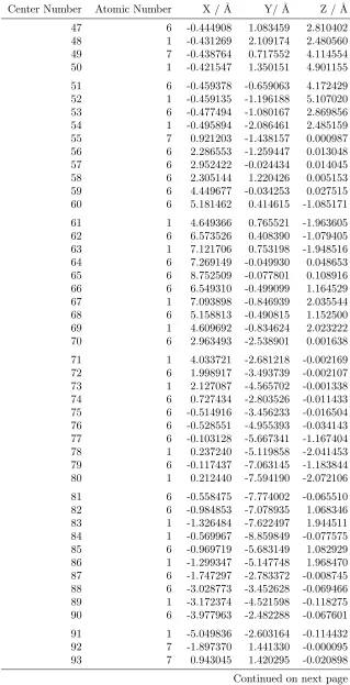
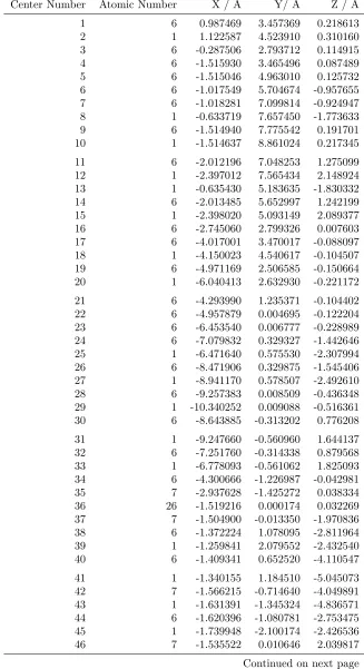
Table 1.7: Optimized Cartesian coordinates of theFeIIIPhCO–₂ molecule

1 6 2.063901 3.447332 0.079828

2 1 2.206164 4.515452 0.135018

3 6 0.783962 2.789153 0.014438

4 6 -0.441389 3.467466 0.021413

5 6 -0.428342 4.965423 0.043228

6 6 0.016390 5.692989 -1.071868

7 6 0.029354 7.088415 -1.051338

8 1 0.372679 7.635569 -1.924207

9 6 -0.400711 7.777865 0.084403

10 1 -0.389870 8.863490 0.100307

11 6 -0.844516 7.064200 1.199714

12 1 -1.176826 7.592208 2.088505

13 1 0.347735 5.161135 -1.958727

14 6 -0.858860 5.668801 1.179286

15 1 -1.200520 5.117823 2.050448

16 6 -1.676654 2.808877 0.011743

17 6 -2.947243 3.488748 -0.004174

18 1 -3.073581 4.560227 -0.011125

19 6 -3.910129 2.532308 -0.005071

20 1 -4.980635 2.666791 -0.007257

21 6 -3.240278 1.256052 -0.008730

22 6 -3.912803 0.029712 -0.014434

23 6 -5.411658 0.040246 -0.034442

24 6 -6.109262 0.434510 -1.186746

25 1 -5.553634 0.730119 -2.071715

26 6 -7.504910 0.442479 -1.204728

27 1 -8.029308 0.746622 -2.105692

28 6 -8.223611 0.057227 -0.070967

29 1 -9.309323 0.063844 -0.085034

30 6 -7.539300 -0.336707 1.080912

31 1 -8.090567 -0.634577 1.967833

32 6 -6.143663 -0.345799 1.099130

33 1 -5.614813 -0.648563 1.997968

34 6 -3.259799 -1.207086 -0.004966

35 7 -1.896178 -1.415417 0.026256

36 26 -0.467811 0.002403 0.002069

37 7 -0.491767 -0.006921 -2.002898

38 6 -0.428887 1.091288 -2.843615

39 1 -0.359270 2.096582 -2.464383

40 6 -0.469906 0.667266 -4.142533

41 1 -0.444436 1.204039 -5.076534

42 7 -0.558695 -0.706004 -4.082991 43 1 -0.607693 -1.337775 -4.869959 44 6 -0.569634 -1.076787 -2.786858 45 1 -0.633759 -2.101537 -2.461566

46 7 -0.442117 0.011725 2.007483

(49)

47 6 -0.360294 1.081314 2.791480

48 1 -0.296490 2.106101 2.466323

49 7 -0.365199 0.710212 4.087541

50 1 -0.309781 1.341603 4.874386

51 6 -0.453658 -0.663049 4.147133

52 1 -0.473670 -1.200178 5.081062

53 6 -0.501032 -1.086659 2.848314

54 1 -0.571620 -2.091943 2.469354

55 7 0.936895 -1.437453 -0.002120

56 6 2.304347 -1.251115 -0.005187

57 6 2.979200 -0.025106 0.000093

58 6 2.323502 1.211354 0.004824

59 6 4.476720 -0.034441 0.004588

60 6 5.199799 0.405979 -1.116274

61 1 4.661393 0.749017 -1.995728

62 6 6.593969 0.397027 -1.109168

63 1 7.158008 0.731751 -1.973561

64 6 7.308206 -0.046066 0.010357

65 6 8.847374 -0.051436 0.013785

66 6 6.585727 -0.483350 1.126945

67 1 7.143393 -0.822174 1.993883

68 6 5.191482 -0.480466 1.128580

69 1 4.646852 -0.817708 2.006429

70 6 2.973078 -2.527722 -0.020835

71 1 4.043421 -2.661480 -0.034018

72 6 2.010003 -3.483887 -0.007877

73 1 2.136109 -4.555395 -0.003701

74 6 0.739784 -2.803609 -0.007197

75 6 -0.495860 -3.462700 -0.005560 76 6 -0.509047 -4.960917 -0.020054 77 6 -0.092858 -5.669790 -1.158000

78 1 0.238686 -5.123108 -2.035756

79 6 -0.107817 -7.065257 -1.171563

80 1 0.213828 -7.597607 -2.061681

81 6 -0.538218 -7.773466 -0.047532

82 6 -0.954215 -7.078477 1.090037

83 1 -1.286854 -7.621354 1.969700

84 1 -0.549254 -8.859155 -0.058038

85 6 -0.940444 -5.682924 1.103775

86 1 -1.260624 -5.146754 1.992152

87 6 -1.720851 -2.785037 0.002328

88 6 -3.001232 -3.443662 -0.054601 89 1 -3.143569 -4.512350 -0.097495 90 6 -3.948722 -2.471788 -0.058809 91 1 -5.020364 -2.588486 -0.104964

92 7 -1.873410 1.442500 0.005094

93 7 0.959420 1.419987 -0.022491

(50)

94 6 3.011568 2.475596 0.073448

95 1 4.083117 2.590825 0.121601

96 8 9.406957 0.359911 -1.038303

(51)

Table 1.8: Optimized Cartesian Coordinates of theFeIIPhCO₂H molecule

1 6 2.050838 3.457774 0.072409

2 1 2.194236 4.526615 0.123998

3 6 0.769848 2.788161 0.009671

4 6 -0.462272 3.460009 0.016105

5 6 -0.449627 4.959147 0.033336

6 6 -0.005848 5.686930 -1.082684

7 6 0.008459 7.082745 -1.068378

8 1 0.352200 7.626301 -1.943721

9 6 -0.421403 7.777802 0.064143

10 1 -0.410539 8.863658 0.076027

11 6 -0.865130 7.066918 1.181423

12 1 -1.197692 7.597973 2.068678

13 1 0.326429 5.151520 -1.967229

14 6 -0.878660 5.671130 1.165245

15 1 -1.221166 5.123653 2.038454

16 6 -1.704905 2.806247 0.009963

17 6 -2.976845 3.495968 -0.001301

18 1 -3.105198 4.567931 -0.005184

19 6 -3.940764 2.540297 -0.002730

20 1 -5.011473 2.678755 -0.002125

21 6 -3.263428 1.261564 -0.010320

22 6 -3.931080 0.028177 -0.013687

23 6 -5.430704 0.037993 -0.027238

24 6 -6.138465 0.449542 -1.168005

25 1 -5.587377 0.760458 -2.050726

26 6 -7.534443 0.457999 -1.180213

27 1 -8.062944 0.776666 -2.074096

28 6 -8.248937 0.054200 -0.050109

29 1 -9.334884 0.060595 -0.058882

30 6 -7.557611 -0.358103 1.091249

31 1 -8.104184 -0.670912 1.976300

32 6 -6.161633 -0.365975 1.101558

33 1 -5.628459 -0.683935 1.992738

34 6 -3.281957 -1.215074 -0.007282

35 7 -1.919195 -1.415960 0.020104

36 26 -0.488308 0.001882 0.000056

37 7 -0.507308 -0.011646 -2.024700

38 6 -0.496580 1.083944 -2.869813

39 1 -0.477522 2.090219 -2.485101

40 6 -0.514446 0.662868 -4.172400

41 1 -0.513766 1.200001 -5.106986

42 7 -0.536384 -0.713728 -4.114545 43 1 -0.553910 -1.346310 -4.901153 44 6 -0.531282 -1.079643 -2.810387 45 1 -0.546261 -2.105340 -2.480556

46 7 -0.468204 0.015430 2.024736

(52)

47 6 -0.444908 1.083459 2.810402

48 1 -0.431269 2.109174 2.480560

49 7 -0.438764 0.717552 4.114554

50 1 -0.421547 1.350151 4.901155

51 6 -0.459378 -0.659063 4.172429

52 1 -0.459135 -1.196188 5.107020

53 6 -0.477494 -1.080167 2.869856

54 1 -0.495894 -2.086461 2.485159

55 7 0.921203 -1.438157 0.000987

56 6 2.286553 -1.259447 0.013048

57 6 2.952422 -0.024434 0.014045

58 6 2.305144 1.220426 0.005153

59 6 4.449677 -0.034253 0.027515

60 6 5.181462 0.414615 -1.085171

61 1 4.649366 0.765521 -1.963605

62 6 6.573526 0.408390 -1.079405

63 1 7.121706 0.753198 -1.948516

64 6 7.269149 -0.049930 0.048653

65 6 8.752509 -0.077801 0.108916

66 6 6.549310 -0.499099 1.164529

67 1 7.093898 -0.846939 2.035544

68 6 5.158813 -0.490815 1.152500

69 1 4.609692 -0.834624 2.023222

70 6 2.963493 -2.538901 0.001638

71 1 4.033721 -2.681218 -0.002169

72 6 1.998917 -3.493739 -0.002107

73 1 2.127087 -4.565702 -0.001338

74 6 0.727434 -2.803526 -0.011433

75 6 -0.514916 -3.456233 -0.016504 76 6 -0.528551 -4.955393 -0.034143 77 6 -0.103128 -5.667341 -1.167404

78 1 0.237240 -5.119858 -2.041453

79 6 -0.117437 -7.063145 -1.183844

80 1 0.212440 -7.594190 -2.072106

81 6 -0.558475 -7.774002 -0.065510

82 6 -0.984853 -7.078935 1.068346

83 1 -1.326484 -7.622497 1.944511

84 1 -0.569967 -8.859849 -0.077575

85 6 -0.969719 -5.683149 1.082929

86 1 -1.299347 -5.147748 1.968470

87 6 -1.747297 -2.783372 -0.008745 88 6 -3.028773 -3.452628 -0.069466 89 1 -3.172374 -4.521598 -0.118275 90 6 -3.977963 -2.482288 -0.067601 91 1 -5.049836 -2.603164 -0.114432

92 7 -1.897370 1.441330 -0.000095

93 7 0.943045 1.420295 -0.020898

(53)

94 6 3.000715 2.488263 0.068978

95 1 4.072059 2.612752 0.119306

96 8 9.340004 0.376474 -1.020588

97 8 9.401384 -0.465301 1.066228

(54)

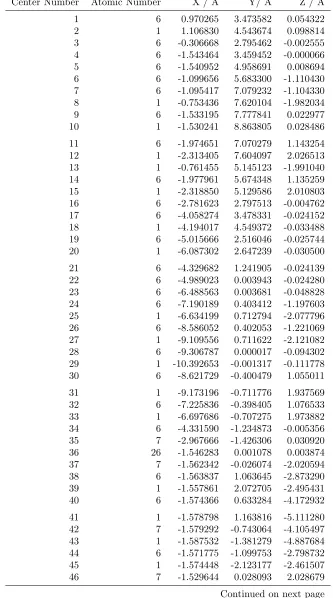
Table 1.9: Optimized Cartesian Coordinates of theFeIIIPh₂CO–₂molecule

1 6 0.987469 3.457369 0.218613

2 1 1.122587 4.523910 0.310160

3 6 -0.287506 2.793712 0.114915

4 6 -1.515930 3.465496 0.087489

5 6 -1.515046 4.963010 0.125732

6 6 -1.017549 5.704674 -0.957655

7 6 -1.018281 7.099814 -0.924947

8 1 -0.633719 7.657450 -1.773633

9 6 -1.514940 7.775542 0.191701

10 1 -1.514637 8.861024 0.217345

11 6 -2.012196 7.048253 1.275099

12 1 -2.397012 7.565434 2.148924

13 1 -0.635430 5.183635 -1.830332

14 6 -2.013485 5.652997 1.242199

15 1 -2.398020 5.093149 2.089377

16 6 -2.745060 2.799326 0.007603

17 6 -4.017001 3.470017 -0.088097

18 1 -4.150023 4.540617 -0.104507

19 6 -4.971169 2.506585 -0.150664

20 1 -6.040413 2.632930 -0.221172

21 6 -4.293990 1.235371 -0.104402

22 6 -4.957879 0.004695 -0.122204

23 6 -6.453540 0.006777 -0.228989

24 6 -7.079832 0.329327 -1.442646

25 1 -6.471640 0.575530 -2.307994

26 6 -8.471906 0.329875 -1.545406

27 1 -8.941170 0.578507 -2.492610

28 6 -9.257383 0.008509 -0.436348

29 1 -10.340252 0.009088 -0.516361

30 6 -8.643885 -0.313202 0.776208

31 1 -9.247660 -0.560960 1.644137

32 6 -7.251760 -0.314338 0.879568

33 1 -6.778093 -0.561062 1.825093

34 6 -4.300666 -1.226987 -0.042981

35 7 -2.937628 -1.425272 0.038334

36 26 -1.519216 0.000174 0.032269

37 7 -1.504900 -0.013350 -1.970836

38 6 -1.372224 1.078095 -2.811964

39 1 -1.259841 2.079552 -2.432540

40 6 -1.409341 0.652520 -4.110547

41 1 -1.340155 1.184510 -5.045073

42 7 -1.566215 -0.714640 -4.049891

43 1 -1.631391 -1.345324 -4.836571

44 6 -1.620396 -1.080781 -2.753475

45 1 -1.739948 -2.100174 -2.426536

46 7 -1.535522 0.010646 2.039817

(55)

47 6 -1.713870 1.069455 2.822555

48 1 -1.876674 2.082256 2.495529

49 7 -1.662132 0.704795 4.119418

50 1 -1.768889 1.330658 4.905365

51 6 -1.441481 -0.653197 4.181377

52 1 -1.361532 -1.183109 5.116218

53 6 -1.364194 -1.074312 2.883282

54 1 -1.197229 -2.069081 2.507245

55 7 -0.105392 -1.430400 0.044587

56 6 1.260159 -1.235443 0.015077

57 6 1.924580 -0.004299 0.028374

58 6 1.261883 1.227374 0.068154

59 6 3.421780 -0.001723 0.012173

60 6 4.126096 0.442424 -1.117215

61 1 3.576688 0.790570 -1.986865

62 6 5.518808 0.444193 -1.136726

63 6 6.263809 0.004821 -0.028109

64 6 5.552392 -0.435474 1.102057

65 1 6.095225 -0.798295 1.969277

66 6 4.159670 -0.439550 1.122422

67 1 3.637060 -0.788219 2.008185

68 6 1.937121 -2.507615 -0.008616

69 1 3.007760 -2.636250 -0.042874

70 6 0.980871 -3.469946 0.033573

71 1 1.114451 -4.540490 0.044116

72 6 -0.293775 -2.798182 0.053715

73 6 -1.525356 -3.463367 0.086550

74 6 -1.531629 -4.961391 0.119900

75 6 -1.135030 -5.706479 -1.001601

76 1 -0.823521 -5.188576 -1.903831

77 6 -1.144187 -7.101688 -0.967250

78 1 -0.837599 -7.662968 -1.844824

79 6 -1.549986 -7.772749 0.188307

80 6 -1.947507 -7.041124 1.309396

81 1 -2.261747 -7.555029 2.212890

82 1 -1.556740 -8.858196 0.214714

83 6 -1.939112 -5.645824 1.275526

84 1 -2.245346 -5.080211 2.150498

85 6 -2.754264 -2.792806 0.074177

86 6 -4.029643 -3.461645 0.016544

87 1 -4.164746 -4.532157 0.016971

88 6 -4.981531 -2.497146 -0.060439

89 1 -6.050894 -2.622317 -0.131180

90 7 -2.931785 1.431430 -0.006371

91 7 -0.102525 1.427576 0.038867

92 6 1.941841 2.492839 0.183917

93 1 3.012260 2.614195 0.244248

(56)

94 6 7.748307 0.004008 -0.050592

95 6 8.455835 -0.303820 -1.227218

96 6 9.848827 -0.307725 -1.243499

97 1 10.394793 -0.554961 -2.148114

98 6 10.587758 -0.004763 -0.093323

99 6 12.125371 -0.013695 -0.115632

100 8 12.699968 0.264560 0.972023

101 8 12.664924 -0.299443 -1.219169

102 6 9.885633 0.304405 1.078096

103 1 10.459852 0.548309 1.965984

104 6 8.492738 0.308960 1.103809

105 1 7.973442 0.575738 2.020284

106 1 7.907571 -0.567592 -2.127539

(57)

Table 1.10: Optimized Cartesian Coordinates of theFeIIPh₂CO₂H molecule

1 6 0.970265 3.473582 0.054322

2 1 1.106830 4.543674 0.098814

3 6 -0.306668 2.795462 -0.002555

4 6 -1.543464 3.459452 -0.000066

5 6 -1.540952 4.958691 0.008694

6 6 -1.099656 5.683300 -1.110430

7 6 -1.095417 7.079232 -1.104330

8 1 -0.753436 7.620104 -1.982034

9 6 -1.533195 7.777841 0.022977

10 1 -1.530241 8.863805 0.028486

11 6 -1.974651 7.070279 1.143254

12 1 -2.313405 7.604097 2.026513

13 1 -0.761455 5.145123 -1.991040

14 6 -1.977961 5.674348 1.135259

15 1 -2.318850 5.129586 2.010803

16 6 -2.781623 2.797513 -0.004762

17 6 -4.058274 3.478331 -0.024152

18 1 -4.194017 4.549372 -0.033488

19 6 -5.015666 2.516046 -0.025744

20 1 -6.087302 2.647239 -0.030500

21 6 -4.329682 1.241905 -0.024139

22 6 -4.989023 0.003943 -0.024280

23 6 -6.488563 0.003681 -0.048828

24 6 -7.190189 0.403412 -1.197603

25 1 -6.634199 0.712794 -2.077796

26 6 -8.586052 0.402053 -1.221069

27 1 -9.109556 0.711622 -2.121082

28 6 -9.306787 0.000017 -0.094302

29 1 -10.392653 -0.001317 -0.111778

30 6 -8.621729 -0.400479 1.055011

31 1 -9.173196 -0.711776 1.937569

32 6 -7.225836 -0.398405 1.076533

33 1 -6.697686 -0.707275 1.973882

34 6 -4.331590 -1.234873 -0.005356

35 7 -2.967666 -1.426306 0.030920

36 26 -1.546283 0.001078 0.003874

37 7 -1.562342 -0.026074 -2.020594

38 6 -1.563837 1.063645 -2.873290

39 1 -1.557861 2.072705 -2.495431

40 6 -1.574366 0.633284 -4.172932

41 1 -1.578798 1.163816 -5.111280

42 7 -1.579292 -0.743064 -4.105497

43 1 -1.587532 -1.381279 -4.887684

44 6 -1.571775 -1.099753 -2.798732

45 1 -1.574448 -2.123177 -2.461507

46 7 -1.529644 0.028093 2.028679

(58)

47 6 -1.520533 1.101650 2.807020

48 1 -1.518429 2.125129 2.470030

49 7 -1.512534 0.744787 4.113728

50 1 -1.504593 1.382914 4.895990

51 6 -1.516862 -0.631556 4.180974

52 1 -1.512078 -1.162230 5.119240

53 6 -1.527476 -1.061735 2.881281

54 1 -1.533117 -2.070769 2.503413

55 7 -0.127217 -1.429254 0.016161

56 6 1.237272 -1.240501 0.022730

57 6 1.895866 -0.001895 0.014080

58 6 1.238838 1.237501 0.001089

59 6 3.394111 -0.001091 0.019280

60 6 4.119800 0.414283 -1.108411

61 1 3.584101 0.743386 -1.993674

62 6 5.512530 0.413744 -1.109095

63 6 6.237188 0.001121 0.022337

64 6 5.510672 -0.411248 1.152691

65 1 6.038873 -0.754634 2.036837

66 6 4.117793 -0.413754 1.149202

67 1 3.580903 -0.742634 2.033816

68 6 1.923062 -2.514890 0.024145

69 1 2.994528 -2.647706 0.021236

70 6 0.965380 -3.476827 0.033269

71 1 1.101120 -4.547819 0.045853

72 6 -0.311147 -2.795844 0.018076

73 6 -1.549295 -3.457234 0.018162

74 6 -1.552740 -4.956525 0.017269

75 6 -1.118092 -5.678744 -1.105998

76 1 -0.778166 -5.139082 -1.985070

77 6 -1.122587 -7.074703 -1.106239

78 1 -0.785590 -7.613707 -1.987018

79 6 -1.563029 -7.775666 0.018575

80 6 -1.998690 -7.070459 1.142593

81 1 -2.339995 -7.606171 2.023718

82 1 -1.566912 -8.861641 0.019080

83 6 -1.993254 -5.674518 1.140940

84 1 -2.329969 -5.131169 2.018948

85 6 -2.786127 -2.792820 0.015423

86 6 -4.062788 -3.471236 -0.045322

87 1 -4.198956 -4.541590 -0.084905

88 6 -5.018558 -2.507410 -0.058068

89 1 -6.089311 -2.636180 -0.109509

90 7 -2.965021 1.431099 -0.008507

91 7 -0.124946 1.428795 -0.024812

92 6 1.926235 2.509870 0.055174

93 1 2.997173 2.639526 0.101530

(59)

94 6 7.720825 0.000717 0.023069

95 6 8.444483 -0.328089 -1.138307

96 6 9.835075 -0.329194 -1.142644

97 1 10.373649 -0.593343 -2.045310

98 6 10.543774 -0.000523 0.022136

99 6 12.027016 0.013470 0.071895

100 8 12.686249 0.295950 1.058538

101 8 12.602216 -0.323725 -1.104135

102 1 13.564460 -0.285607 -0.969435

103 6 9.833872 0.328119 1.185576

104 1 10.386333 0.589792 2.081383

105 6 8.444721 0.328891 1.185198

106 1 7.912481 0.610237 2.087926

107 1 7.911584 -0.609263 -2.040683

108 1 6.042134 0.758615 -1.991816

Table 1.11: Energies (in hartree) for the optimized geometries provided in Tables 1.7-1.10, using the specified DFT functional and basis set.

Species B3LYP|6-31G(d,p) B3LYP|TZVP TEMPO −483.750173 −483.862334 TEMPOH −484.359752 −484.473101

FeIIIPhCO–₂ −3816.774186 −3817.676745

FeIIPhCO₂H −3817.407030 −3818.292971

FeIIIPh₂CO–₂ −4047.838889 −4048.805990

(60)

(61)

Table 1.12 – continued from previous page Atom Name X / ˚A Y/ ˚A Z / ˚A H02 -4.60 12.37 -0.08

H02 4.47 12.40 -0.30

H03 -5.14 8.93 1.80

H03 -5.24 10.53 -2.19

H03 5.12 8.99 1.64

H03 5.04 10.54 -2.36

H04 -7.62 8.93 1.86

H04 -7.72 10.53 -2.13

H04 7.59 8.99 1.60

H04 7.52 10.54 -2.41

H05 -8.92 9.73 -0.11

H05 8.81 9.77 -0.43

H06 -4.59 7.09 -0.29

H06 4.49 7.13 -0.46

H07 -2.67 5.21 -0.33

H07 2.58 5.23 -0.48

H08 0.67 4.58 1.63

H08 -0.75 4.68 -2.42

H09 0.68 2.11 1.57

H09 -0.74 2.21 -2.49

H10 -0.02 0.91 -0.49

H13 -2.14 9.87 2.20

H13 2.03 9.64 -2.77

H14 -1.35 9.83 4.60

H14 1.24 9.69 -5.18

H15 1.19 9.69 4.78

H15 -1.30 9.83 -5.36

H16 2.06 9.64 2.16

H16 -2.17 9.87 -2.74

N01 1.37 11.17 -0.29

N01 -1.49 11.16 -0.28

N02 -1.48 8.33 -0.29

N02 1.38 8.34 -0.30

N03 -0.05 9.75 1.72

N03 -0.06 9.75 -2.30

N04 -0.73 9.79 3.80

(62)

(63)

Table 1.13 – continued from previous page Atom Name X / ˚A Y/ ˚A Z / ˚A H02 -4.66 -34.88 -0.55 H02 4.41 -34.95 -0.22 H03 -5.18 -31.36 -2.35 H03 -5.31 -33.10 1.58 H03 4.99 -31.61 -2.34

H03 5.06 -33.01 1.72

H04 -7.65 -31.34 -2.43 H04 -7.79 -33.08 1.50 H04 7.47 -31.62 -2.39

H04 7.53 -33.02 1.68

H05 -8.97 -32.20 -0.50 H05 8.75 -32.32 -0.38 H06 -4.63 -29.60 -0.16 H06 4.44 -29.67 -0.22 H07 -2.70 -27.73 -0.44 H07 2.55 -27.77 -0.98 H08 0.51 -27.03 -2.07 H08 -0.66 -27.31 2.05 H09 0.53 -24.56 -1.90 H09 -0.64 -24.84 2.23 H10 -0.04 -23.45 0.25 H13 -2.17 -31.91 -2.74

H13 1.97 -32.06 2.22

H14 -1.40 -32.04 -5.14

H14 1.20 -32.15 4.62

H15 1.11 -32.47 -5.33 H15 -1.33 -32.42 4.81 H16 1.97 -32.63 -2.71 H16 -2.21 -32.51 2.20 N01 1.31 -33.70 -0.25 N01 -1.55 -33.68 -0.27 N02 -1.53 -30.85 -0.23 N02 1.33 -30.87 -0.26 N03 -0.11 -32.27 -2.26 N03 -0.11 -32.28 1.75 N04 -0.79 -32.15 -4.35

(64)

(65)

Table 1.14 – continued from previous page Atom Name X / ˚A Y/ ˚A Z / ˚A

H02 4.51 12.36 -0.49

H02 -4.58 12.43 -0.26

H03 5.03 8.92 -2.38

H03 5.13 10.51 1.61

H03 -5.24 9 -2.19

H03 -5.14 10.57 1.80

H04 7.50 8.91 -2.44

H04 7.60 10.5 1.56

H04 -7.71 9.01 -2.14