a solid-shell element for use in
sheet deformation processes
and the EAS method
Wouter Quak
25-05-2007
Master Thesis
Mechanics of Forming Processes Department of Mechanical Engineering
Contents
Summary vii
Samenvatting ix
Preface xi
Nomenclature xiii
1 Introduction 1
1.1 Background . . . 1
1.2 Problem definition . . . 2
2 Solid-shells 3 2.1 Introduction . . . 3
2.2 Literature review . . . 3
2.3 Element selection . . . 4
3 Basic theory 7 3.1 Introduction . . . 7
3.2 Locking phenomena . . . 7
3.2.1 Introduction . . . 7
3.2.2 Shear locking . . . 8
3.2.3 Volumetric locking . . . 9
3.2.4 Thickness locking . . . 10
3.2.5 Constraint counting . . . 10
3.2.6 Subspace methodology . . . 11
3.3 Mixed formulations . . . 12
3.3.1 Introduction . . . 12
3.3.2 Irreducible . . . 13
3.3.3 Mixed u−ε−σ form . . . 13
3.4 EAS method . . . 15
iv CONTENTS
3.5 EAS method in non-linear situations . . . 17
4 Simo-Rifai quadrilateral 19 4.1 Introduction . . . 19
4.2 Formulation . . . 19
4.2.1 Enhanced strain parametrization . . . 19
4.2.2 Coordinate transformation . . . 20
4.3 Simulations . . . 22
4.3.1 Introduction . . . 22
4.3.2 Patch test . . . 22
4.3.3 Mesh distortion . . . 23
4.3.4 Cook’s membrane . . . 23
4.3.5 Bending process . . . 26
4.4 Conclusions . . . 28
5 ‘RESS’ 3d solid-shell 31 5.1 Introduction . . . 31
5.2 Formulation . . . 31
5.2.1 Introduction . . . 31
5.2.2 EAS implementation . . . 32
5.2.3 Coordinate systems . . . 33
5.2.4 Coordinate transformation . . . 35
5.2.5 Enhanced strain parametrization . . . 36
5.2.6 Reduced integration . . . 37
5.2.7 Stiffness computation . . . 38
5.2.8 Stabilization procedure . . . 39
5.2.9 Incremental procedure . . . 42
5.3 Simulations . . . 44
5.3.1 Introduction . . . 44
5.3.2 Clamped square plate . . . 45
5.3.3 Cube stretching . . . 47
5.3.4 Strip bending . . . 49
5.4 Conclusions . . . 52
6 Conclusions and recommendations 53
Appendices 55
A Coordinate transformations 57
CONTENTS v
Summary
Sheet deformation processes can be simulated by using the finite element method. The used finite elements for simulation of these processes in 3 di-mensions are mostly shells. These elements are suited for situations in which in-plane dimensions are considerably larger than the thickness dimension.
Recently a new group of elements has been introduced named ‘solid-shells’. These elements are a mixture between solid bulk elements and shells and try to take the benefits of both sides. Goal of this research is investi-gating and developing a solid-shell element for use in the in-home developed software packageDiekAof the Mechanics of Forming Processes group at the
University of Twente.
First the general background of the solid-shell is investigated. The locking phenomena that prevent the use of standard solid bulk elements in thin walled geometries are treated. These locking phenomena can be especially present in low thickness geometries. One of the most important methods to alleviate several types of locking is the EAS (Enhanced Assumed Strain) method.
To get familiar with the EAS method, an element was programmed. This 2d linear quadrilateral contains extra internal modes of deformation due to the EAS method. Several tests were performed in which the element shows very good performance in bending and incompressible situations with respect to the standard quadrilateral. Finally a non-linear simulation of a ‘free-bending’ deformation process showed that less EAS elements could be used to give the same performance as would be the case with standard not-enhanced quadrilaterals.
Scanning literature revealed an interesting solid-shell element, named ‘RESS’. The base of the element is a 3d linear 8 node hexagonal. Several methods are used to get good shell performance of this element. These are: reduced integration in in-plane directions accompanied by a physical stabi-lization procedure, the EAS method and a B-bar method. The element was programmed both linear and geometric non-linear in C++ with aid of the FeaTure toolbox. The element is tested first in a geometric linear
viii SUMMARY
walled problem. The performance is very good especially in incompressible situations. Secondly the geometric non-linear situation is tested. A simula-tion of the bending of a strip shows good comparison with shell elements.
Samenvatting
Plaat-vervormingsprocessen kunnen succesvol worden gesimuleerd met be-hulp van de eindige elementen methode. De gebruikte elementen voor sim-ulatie van deze processen zijn veelal shell elementen. Deze elementen zijn geschikt voor situaties waarin de dikte van de plaat aanzienlijk kleiner is dan de afmetingen in het vlak.
Onlangs is er een nieuwe groep elementen ge¨ıntroduceerd genaamd “solid-shells”. Deze elementen zijn een mix tussen solid bulk elementen en shell elementen en proberen de voordelen van beide zijden te benutten. Doel van dit project is het onderzoeken en ontwikkelen van een solid-shell element voor het gebruik in het programma DiekA van de Mechanics of Forming
Processes groep op de Universiteit van Twente.
Ten eerste is de algemene achtergrond van solid-shell elementen onder-zocht. De locking verschijnselen, die voorkomen dat solid elementen kunnen worden toegepast voor dunwandige vormen, worden toegelicht. Een van de meest belangrijke methodes om locking tegen te gaan is de EAS (Enhanced Assumed Strain) methode.
Teneinde bekend te geraken met deze EAS methode is een eindig ele-ment geprogrammeerd. Dit 2d lineaire 4 knoops eleele-ment bevat extra interne vervormings mogelijkheden door de EAS methode. Verscheidene tests zijn uitgevoerd waarin het element goede resultaten laat zien. Vooral in buiging gedomineerde- en incompressibele problemen presteert het element beter in vergelijk met een standaard 4 knoops element. Uiteindelijk wordt het ele-ment in een niet-lineair kant proces getest. Minder EAS eleele-menten kunnen worden gebruikt in vergelijk met standaard elementen.
Scannen van literatuur bracht een interessant solid-shell element aan het licht genaamd ‘RESS’. Het element heeft als basis een 3d lineaire 8 knoops kubus. Verscheidene methodes worden toegepast om goede shell capaciteiten te cre¨eren. Deze zijn: gereduceerde integratie vergezeld met een stabilisatie procedure, de EAS methode en een B-bar methode. Het element is lineair en geometrisch niet lineair geprogrammeerd in C++ met behulp van de
x SAMENVATTING
Ture toolbox. Ten eerste is RESS getest in een dunwandig probleem. Het
element laat goede resultaten zien, met name in incompressibele situaties. Ten tweede is het element getest in het geometrisch niet lineair buigen van een strip. Resultaten komen goed overeen met resultaten uit de literatuur en met standaard shell elementen.
Preface
In the following two paragraphs I would like to thank people who supported me during my master thesis.
First I would like to thank the group of applied mechanics for the good working atmosphere and for drinking cubic hecto-gallons of coffee during the nine months.
I would like to thank Han Hu´etink for helping me out with tensor transfor-mations and Ron Peerlings of the University of Eindhoven and Bert Geijselaers of the University of Twente for taking place in my exam commission. A spe-cial thanks goes out to Ton van den Boogaard as my daily supervisor for always making time and giving great guidance to the project.
Nomenclature
Roman
A mixed field matrix b volume force vector
B strain-displacement interpolation matrix C mixed field matrix
D constitutive matrix e cartesian base vector E Young’s modulus E Green-Lagrange strain f force vector
F coordinate transformation matrix F deformation gradient
g natural co- or contravariant base vector G mixed field matrix
J Jacobi matrix K stiffness matrix
N field interpolation matrix p orthonormal coordinate vector q degree of freedom vector r orthonormal base vector
R rotation part of deformation gradient S second Piola-Kirchhoff stress
S spatial derivative matrix t traction force vector
T coordinate transformation matrix u displacement vector
U stretch part of deformation gradient x cartesian coordinate vector
xiv NOMENCLATURE
Greek
α enhanced strain parameter vector γ boundary of current analysis domain Γ boundary of reference analysis domain
ε linear strain ν Poissons ratio
ξ natural coordinate vector
σ linear stress
ω internal current analysis domain Ω internal reference analysis domain
Accents
Chapter 1
Introduction
1.1
Background
For some decades now, sheet deformation processes can be successfully simu-lated with the finite element method. During sheet forming various forms of deformation take place within the sheet, for instance membrane stretching, bending and shear.
Most FEM calculations in sheet deformation processes use shell elements. Although successful in a lot of cases there are some drawbacks of these el-ements. First of all the elements use rotational degrees of freedom. The rotational degrees of freedom have to be updated after iterations and the proper way to handle the rotations at the boundaries is not straightforward. To connect a shell with a bulk element, special transition elements are re-quired. Plane stress assumptions yield that thickness is updated after the finite element iteration. Double sided contact is difficult to model.
Currently there are developments for using solid bulk elements for sheet deformation processes. Certain aspects of a solid formulation give benefits over the shell elements. These are: full constitutive law, double sided contact, easy mesh generation, no rotational degrees of freedom and above all; fast computation.
The problem however with these simple, computational friendly elements is their locking behavior and inability to conform to certain deformation modes. These locking phenomena prevent solid elements to be used for ‘shell-like’ geometries. Locking occurs when, due to such particulars as displace-ment interpolation used and integration rule chosen, a physically realistic displacement mode tends to be “locked out” of element response because the mode activates extraneous strains that require much higher energy input than do strains of the realistic mode.
2 CHAPTER 1. INTRODUCTION
Various methods are available to counter the locking phenomena. Well known are for instance the method of reduced integration and the B-bar method. A new innovation is the enhancement of the strain field, also known as EAS. With this technique internal degrees of freedom are generated which will alleviate this locking behavior. The method does not produce disad-vantageously artifacts like for instance the hourglass modes resulting from a reduced integration procedure. The solid elements which are modified in order to be suited for shell geometries are called solid-shells.
1.2
Problem definition
Analyze current developments involving the use of simple solid elements in sheet deformation processes. Scan the literature for publications on recently developed solid-shell elements. Implement a solid-shell element with in mind that the final application in which the element should function is the ‘in-house’ developed software programDiekA. The finite element toolbox Fea-TureinC++ should be a good tool for element development. The element
Chapter 2
Solid-shells
2.1
Introduction
As described in Chapter 1, a solid-shell is a linear 3d solid with capabilities to perform shell like calculations. The 3d solid is modified in such a fashion that shell like properties, mostly bending and in plane stretching, can be efficiently modeled. Main part is to get rid of the locking phenomena which prevent ‘unmodified’ linear solids in thin walled applications. Various approaches are available to obtain the desired behavior. Especially the EAS method is suited to prevent the locking phenomena thus making it a good tool to make solid-shell elements.
The applied methods for good shell performance of a solid element need to enhance element properties in for instance a single direction. This makes that solid-shell elements in general show different behavior in thickness di-rection than in in-plane didi-rection. Drawback of this non-symmetric behavior is that element numbering has to be in a specific manner in order to guar-anty element orientation in the way it is intended to. Just meshing like with ‘normal’ 3d elements is not sufficient.
2.2
Literature review
Below a short summary of recent developments of solid-shell elements as found in literature.
The solid-shell concept was introduced by Hauptmann and Schweizerhof in 1998 [21]. Several solid-shells are introduced. All elements make use of the Assumed Natural Strain (ANS) method. Two methods are used to initialize a variable strain in thickness direction. One is adding a quadratic interpolation
4 CHAPTER 2. SOLID-SHELLS
in thickness direction, the other uses the EAS method for this purpose. The elements show good comparisons with shells.
Hauptmann and Schweizerhof extended their solid-shell concept further in 2000 [17]. The extension to large deformations, plasticity and hyper-elasticity is made. Since incompressibility is often present in plasticity, the volumetric locking phenomenon is analyzed for the solid-shell elements.
Harnau and Schweizerhof reviewed the solid-shell concept in their article [20] published in 2002. Locking phenomena are elaborated. Various tech-niques to prevent locking are reviewed.
In 2003 Areias, C´esar de S´a and Concei¸c˜ao Ant´onio propose the ‘His’ element [2]. The element uses merely the EAS method to counter all locking phenomena. The element is suited for solid and shell analysis. The element is computationally inefficient but gives good results.
In 2003 a group from the university of Aveiro in Portugal produced an article [11] on two elements, named HCiS12 and HCiS18. The elements are based on a 3d linear hexahedron and use an EAS formulation with 12 or 18 parameters respectively. As noted by themselves, introducing 12 or 18 new degrees of freedom will have its effect on computation time. The fact that 2x2x2 integration is used will also not enhance its computational friendliness. In 2004 the same group announce another element named ‘RESS’ with the following properties: reduced integration, EAS and physical stabilization [14]. The reduced integration is 1x1 in-plane and an undefined amount of integration points along thickness. The results seem very good and especially the integration scheme can be beneficial for plasticity. The article treats only the geometric linear case. Various linear test examples are given.
In the article [15] in 2005 ‘RESS’ was upgraded for geometrically non-linear applications. Several results of ‘well-known’ large deformation prob-lems are given and compared with results of other authors.
The last article [16] on the element was published in 2007. The arti-cle introduces more results of problems, including several forming processes. These are; bulging of a plate under a uniform pressure, deepdrawing of a thin walled cup; in special the earing phenomena, hydroforming of a square tube and unconstrained cylindrical bending (free-bending). The in-plane reduced integration scheme is evaluated.
2.3
Element selection
2.3. ELEMENT SELECTION 5
seem very promising. Second, the element is published in three articles. The functioning is treated elaborately. The fact that first the linear variant is treated and in the second article the geometric non-linear situation can have didactic benefits. At last, the element incorporates an unspecified number of integration points in through thickness direction, which should give good results in plasticity.
In the following chapter, the fundamentals necessary to understand a solid-shell are explained. First the problems (the locking phenomena) are elaborated. In the second part of chapter 3 the EAS method is explained.
The EAS method must be mastered in order to create a solid-shell ele-ment. Therefore a simple 2d linear enhanced element is programmed. Chap-ter 4 treats this development. Various tests are introduced and the function-ing of the EAS method for this specific element is reviewed.
Chapter 3
Basic theory
3.1
Introduction
In this chapter the basic theory that is needed to understand the functioning of solid-shell elements in general is treated.
First the locking phenomena which make standard linear bulk elements not suited for shell calculations are treated. Two tools to analyze the lock-ing phenomena are introduced. The constraint countlock-ing method and the subspace method.
In section 3.4 the EAS method is derived. To introduce the EAS method, mixed formulations are treated in the preceding section 3.3. The EAS method is based on a specific three field mixed method. Afterwards the derivation to the EAS method is made. Specific element dependent properties are treated later on in the following chapters.
The derivations presented below are for linear elasticity unless stated otherwise.
3.2
Locking phenomena
3.2.1
Introduction
The most important locking problems will be briefly explained below. The linear 4 node plane strain quadrilateral is used to illustrate the locking phe-nomena. The natural coordinates are chosen identical to the global cartesian coordinates, so no mapping has to be done (Equation 3.1). Standard ‘full’ integration is the numerical integration scheme that would be exact if the
8 CHAPTER 3. BASIC THEORY
element is not deformed. In case of the linear quadrilateral this is 2x2.
J =1 (3.1)
3
1 2
4
x, ξ y, η
x=ξ, y =η
Figure 3.1: The 4 node quadrilateral
3.2.2
Shear locking
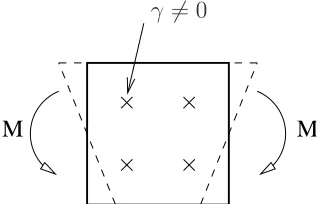
M M
γ 6= 0
Figure 3.2: deformation during bending
Transverse shear locking or trapezoidal locking is the inability of the element to reproduce a null transverse (in thickness direction) shear strain energy state in pure bending. Most linear bulk elements suffer from this lock-ing. Figure 3.2 shows an element subjected to a moment. The displacement vector of a bending moment could be the following:
3.2. LOCKING PHENOMENA 9
Due to the formulation of theB-matrix, shear strains will be triggered when a displacement of Equation 3.2 is used.
Equation 3.3 shows that the terms in the B-matrix for εxy will not be zero when the element is subjected to a moment, like in Figure 3.2. So by using full integration of the B-matrix at four points, the shear strain terms will be added four times. To ensure zero shear strains, it is an option to use reduced integration. The shear strains at point x = 0, y = 0 are used and these are indeed zero in this case as can be seen with Equation 3.3. Drawback of this approach is the introduction of deformation modes that will cost no energy (spurious modes).
3.2.3
Volumetric locking
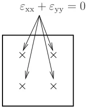
εxx +εyy = 0
Figure 3.3: constraints at integration points
Volumetric locking occurs when constitutive behavior is incompressible or nearly incompressible. An implicit constraint is introduced at the integration points. Figure 3.3 shows the equation at the integration points which should be obeyed by the interpolation. This implicit constraint can be made clear by filling in the constitutive matrix for plane strain in incompressibility.
10 CHAPTER 3. BASIC THEORY
TheDwill act as an implicit constraint having its effect on the stress and thus on the potential energy.
To prevent high stresses;
εxx+εyy = 0 (3.10)
If the nodal degrees of freedom can not satisfyεxx =−εyy at an integration point a high stress will be accounted for, indirect giving a large stiffness. If the 4 node quadrilateral has 8 degrees of freedom, then a certain number of these degrees of freedom are ‘occupied’ by satisfying constraint 3.10.
3.2.4
Thickness locking
If a thin plate is being bend, the strains in in-plane direction vary linearly over the thickness direction. The stress in thickness direction should be near zero, as is usual in thin plate problems. The strain in thickness direction should vary over the thickness to achieve this. Due to coupling of out-of-plane stresses and in-plane strains, locking occurs. The y-direction is along the thickness. The x-direction is in in-plane direction.
σyy =
E
(1 +ν)(1−2ν)(νεxx+ (1−ν)εyy) (3.11)
In this bending situation σyy should be equal to zero. So if εxx is a function of y then soεyyshould be, in order to getσyyzero all over the domain if full integration was used.
3.2.5
Constraint counting
Constraint counting is a rule of thumb, to get an indication whether an element will show locking behavior. The constraint ratio is the number of active degrees of freedom divided by the constraints.
r = ndof
ncons (3.12)
3.2. LOCKING PHENOMENA 11
In case of volumetric locking, 4 constraints are applied at the integration points (3.10). So if the 2d 4-node element is supported with a minimal number of degrees of freedom, in this case 3, then 8−3 = 5 active degrees of freedom remain.
r= 5
4 >1 (3.13)
Probably no locking occurs. Adding one more support could give locking. For large meshes the total number of active degrees of freedom and constrains are considered. For instance the situation of Figure 4.3 in Chapter 4 can be analyzed as follows:
r= 40
64 <1 (3.14)
Locking will occur as will be pointed out in Figure 4.4(b). Using reduced integra-tion (1x1) will give:
r= 40
16 >1 (3.15)
No locking will be present.
3.2.6
Subspace methodology
The subspace method is a method to prove how many degrees of freedom are indeed needed to satisfy implicit locking constraints [3, 11]. The constraint counting method is indicative, the subspace method is exact. For instance in incompressible situations, the number of deformation modes that are not within the total element response because of the constraint can be determined exactly.
The approach to calculate the subspace is to write the constraints as functions of the displacements for each integration point. Below the subspace analysis of the 2d quadrilateral for the volumetric locking phenomena is presented. The constraint is written as a function of the nodal displacements for all four integration points.
∂ u
This equation should hold at all four integration points.
12 CHAPTER 3. BASIC THEORY
Where:
a= 1 3
√
3 (3.19)
The rank of this matrix is three, so three linear combinations of the nodal displace-ments, or better, three modes of deformation are needed to satisfy the constraint. Therefore these modes will be locked out of response of the total subset of possible solutions. As shown by C´esar de S´a and Natal Jorge [3], the plane strain 4 node element should supply 7 modes of deformation in incompressible situations. The only mode that should not be present in the total set of possible solutions is the outwards or inwards movement of the element’s edges collectively. The deforma-tion mode is visualized in Figure 3.4. The dashed line is the deformed state, the continuous line the reference state. By using reduced integration (1x1), Equation
Figure 3.4: compressible deformation mode
3.18 will become:
£
−1 1 1 −1 −1 −1 1 1 ¤
u=0 (3.20)
This matrix has a rank of one. The linear combination of the nodal displacements corresponds with the deformation mode displayed in Figure 3.4. The approach for the subspace analysis for the other locking phenomena is similar to the presented volumetric locking subspace method.
3.3
Mixed formulations
3.3.1
Introduction
The set of differential equations from which the discretization procedure starts determines whether the formulation is called mixed or irreducible. For both the irreducible and mixed formulations, the starting point is the weak form of equilib-rium:
Z
Ω
δεTσdΩ− Z
Ω
δuTbdΩ− Z
Γ
3.3. MIXED FORMULATIONS 13
3.3.2
Irreducible
The usual approach for continuum mechanical finite element analysis is to create a potential energy function which contains only displacement terms. Stresses and strains are written as functions of the displacements. The formulation in which no further elimination of variables can be made is called ‘irreducible’. The following relations are used in a strong form, and thus holding for all particles within the finite element.
σ =Dε (3.22)
ε=Su (3.23)
This will give the well known ‘irreducible’ form for linear elasticity:
Π(u) =
The potential energy is only a function of the displacements.
u=Nuu˜ (3.25)
Bu=SNu (3.26)
δu=Nuδu˜ (3.27)
The other two variables are already expressed as functions ofu. Making a Taylor series of this potential;
Π(˜u+δu˜) = Π(˜u) +∂Π(˜u)
Equilibrium is demanded for arbitrary virtual displacement fields for the first linear coefficient.
∂Π(˜u)
∂u˜ =0 ∀ δu˜ (3.29)
The final discretized equation for the finite element analysis will become;
Z
This form is only a function of the displacements.
3.3.3
Mixed
u
−
ε
−
σ
form
14 CHAPTER 3. BASIC THEORY
well known in incompressible situations is theu−pform, relieving the volumetric locking constraint. Another interesting mixed formulation is the u−σ form as used in Pian-Sumihara’s element.
Mixed formulations contain variables that could be eliminated by substitution in a strong form. For instance a three field mixed form still contains all three variables: displacement, strain and stress. The equations 3.22 and 3.23 that link the variables are used in a weak form.
Z
The equation of weak equilibrium 3.21 now is:
Z
The corresponding potential energy function is:
ΠHW(u,ε,σ) =
This variational principle is also known by the name of Hu-Washizu. Note that to get the finite element equations 3.31, 3.32 and 3.33 the potential energy has to be differentiated to all three variables.
˜
A discretization has to be made for all three variables whereas with the irreducible form only the displacement had to be discretized.
ε=Bε˜ε (3.37)
σ=Nσσ˜ (3.38)
δu=Nuδu˜ (3.39)
δε=Bεδε˜ (3.40)
δσ=Nσδσ˜ (3.41)
3.4. EAS METHOD 15
3.4
EAS method
The EAS formulation was introduced in 1990 by J.C. Simo and M.S. Rifai [19]. With this technique, various types of locking can be avoided, for instance volu-metric locking or transverse shear locking. Main point of the method is the en-hancement of the displacement based strain field. The construction of the added enhanced strain field will decide which type(s) of locking can be prevented. Start-ing point for the EAS method is the three-field mixed formulation of Hu-Washizu as presented in the previous section.
With the enhanced assumed strain method the total strain field is assumed to consist of the displacement based strain field and an assumed additive strain field. This enhanced strain field can contain modes that are not present in the displacement interpolation.
ε=S u+εen (3.42)
Thus requiring the stationarity to all its variables:
Πen(σ,εen,u) =
Variation of the potential energy principle will yield three integrals which have to be satisfied by the fields.
Z
Prescribing functions within the element for the enhanced strain field:
εen=Benα (3.47)
Displacements are continuous between elements. Enhanced strains and stresses are not. The three integrals above will give a linear system of equations:
16 CHAPTER 3. BASIC THEORY
The internal force vectors are set to zero since no prestressing effects are considered. Therefore f1 and f2 are zero and f3 consists only of the external force vector. In iterative-incremental procedures the internal force vectors can not be set to zero.
The system of equations above should comply to the stability condition for mixed formulations. The stability condition prevents the matrix system of Equa-tion 3.48 to become singular [22]. The vector of variables, nen,nσ and nu are the number of unknowns in the vector of enhanced strains, stresses and displacements respectively. The following inequality should be met:
nu+nen≥nσ (3.56)
The choice for Ben is subject to two conditions. Condition one tells that the introduced strains ofBen andBu should be different from each other.
Ben∩Bu =∅ (3.57)
Ignoring this condition will give matrix singularity and thus non-unique solutions. Also would it give no further benefit to add a deformation mode with the enhanced strain matrix which is already present in the displacement based strain. All en-hanced parameters or columns ofBen should be independent.
A second condition is invoked to get rid of Nσ. Matrix Ben is chosen orthogonal to matrixNσ. The effect of this is that matrixCequals zero and can be removed from the total system of equations.
C=
Z
Ω
BTenNσdΩ = 0 (3.58)
3.5. EAS METHOD IN NON-LINEAR SITUATIONS 17
be removed from the total matrix system if:
Z
Ω
BTendΩ = 0 (3.59)
The number of variables is now down to two. The new linear system of equa-tions:
The reduced system of equations is used to determine a new stiffness matrix. Therefore the enhanced strain parameters are condensed out at element level.
K∗u˜ =f
3 (3.61)
K∗ =K−GTA−1G (3.62)
To obtain the local stiffness matrix, matrix Amust be invertible.
The static condensation of the enhanced strain parameters gives several ben-efits. First, the element stiffness matrix has still the same size (same amount of degrees of freedom), therefore the assembly of the element stiffness matrices is the same as was before for the not enhanced element. Secondly the total, global, stiff-ness matrix is not extended, thus still the same effort has to be done for solving the system. A linear enhanced element should be in almost every case (if Ben is not too large) be computationally more efficient than its quadratic version, while quadratic elements can still introduce their own locking problems.
The enhanced strain parameters can be calculated after solvingKu˜ =f. With the known nodal displacements, the strains (and thus the stresses) can be deter-mined as follows:
α=−A−1Gu˜ (3.63)
ε=Buu˜+Benα (3.64)
With these parameters and the nodal displacements it is possible to calculate the ‘total’ strain and stress. The definition ofBendictates the ability of the formulation to alleviate distinct locking phenomena. Various approaches are found in literature. In further chapters the subscript u of the Bu- and Nu- matrices will be discarded for readability.
18 CHAPTER 3. BASIC THEORY
n as the incremental counter. The internal force vectors can not be discarded as was the case in the linear situation (Equation 3.60).
fuint= Z
ω
BTσdω (3.65)
fenint= Z
ω
BTenσdω (3.66)
Linearization of these force vectors will give a very similar system as seen in Equa-tion 3.60.
·
A G
GT K
¸ µ i+1
iα i+1
iu˜
¶ =
µ
−fenint
fuext−fuint
(3.67)
The static condensation procedure will yield:
£
K−GTA−1G¤i+1
iu˜ =fuext−fuint+GTA−1fenint (3.68) The system of Equation 3.68 is build and solved for each iteration until the com-plete right hand side is zero. For every iteration:
i+1u˜ = iu˜+ i+1
iu˜ (3.69)
i+1α= iα+ i+1
iα (3.70)
i+1
iα=−iA−1 iGi+1iu˜− iA−1ifenint (3.71) The strain over the increment can be calculated with:
n+1
nε= nBn+1nu˜+ nBenn+1nα (3.72)
To increase the accuracy of the calculated strains, the strain is often calculated by using the geometry at the half of the increment:
n+1
nε= n+1/2Bn+1nu˜+ n+1/2Benn+1nα (3.73)
Chapter 4
Simo-Rifai quadrilateral
4.1
Introduction
The Simo-Rifai 4-node element is an extension of a normal 2d linear 4 node quadri-lateral. As shown in Chapter 3, this quadrilateral suffers from shear locking in bending dominated situations and volume locking in incompressible situations. Therefore an enhanced strain field is introduced which will alleviate this locking behavior. The stress state is plane strain.
The following sections will only treat element dependent properties; enhanced strain parametrization and transformation of this parametrization. All other oper-ations at the element are general for finite EAS elements and are according Chapter 3.
The linear version of the element is programmed inC++ with theFeaTure
toolbox. The non-linear variant was programmed inDiekA.
4.2
Formulation
4.2.1
Enhanced strain parametrization
The enhanced strain parametrization in the natural coordinate system:
˘
Why the matrix is formulated this way can be made clear when the global coor-dinate system is chosen identical to the local natural system. For an element the
20 CHAPTER 4. SIMO-RIFAI QUADRILATERAL
total strain of a particle within the element will become;
ε=S u+εen (4.3)
The first normal strain is enhanced with an extra function in x direction. The same holds for the second normal strain εyy. The normal strains are enhanced so the two introduced parameters α1 and α2 can be used to alleviate volumetric locking or thickness locking.
The shear strains are given two extra degrees of freedom α3 andα4 as a func-tionsx andy respectively. These parameters are used to get rid of the extraneous shear strains (shear locking).
When using the method of constraint counting, one would suspect that 8 de-grees of freedom should be introduced; 4 integration points, 2 constraints per integration point. A subspace analysis on the other hand shows that the subspace of the constraints (volumetric- and shear locking) still has a rank of 4, thus not 8. The 4 introduced parameters are indeed sufficient to get all 7 deformation modes belonging to a 4 node linear element in incompressibility.
4.2.2
Coordinate transformation
The enhanced strains are prescribed in the natural coordinate system as a func-tion of the natural coordinates. To calculate the integrals over the element, the enhanced strains in the global coordinate system have to be known. The strain, a second order tensor, has to be projected on the global domain. Appendix A con-tains a derivation of the projection of an arbitrary second order tensor. In general, FEM software uses matrix vector notation, so the following derivation will end in that form. In tensor notation a projection of a second order tensor yields:
[εen] = j0 j(ξ, η)[T]
T[˘ε
en] [T] (4.5)
And in matrix vector notation:
4.2. FORMULATION 21
There are two options for the definition of T. The direction of the enhanced strain can be chosen in direction of the covariant or contravariant base vectors. See Appendix A for more details. Definition of the enhanced strain in direction of the covariant base vectors gives the following transformation:
T=J0 (4.9)
Choosing a contravariant set of base vectors yields:
T=J-T0 (4.10)
Equations 4.9 and 4.10 are the only two transformations which will guarantee frame invariance. Renumbering the nodes, but keeping a certain order though, should have no difference on outcomes whatsoever. The last option 4.10 seems more effective considering mesh distortion sensitivity so this one is used for the projection of the enhanced strain field [22]. J0 is the Jacobi matrix atξ, η = 0,0.
If the mapping is done with the complete Jacobi matrix as a function of the natural coordinates, the patch test will not be satisfied. The linear enhanced strain functions in the isoparametric local space will be higher order functions in the global space due to the introduction of extra functions in the Jacobi matrix. Equation 3.58 can not be guaranteed zero.
The j0 term can be discarded when programming EAS elements, since it will only scale the parameters altogether. When calculating strains and stresses after-wards, the elimination of j0 also has to be made.
22 CHAPTER 4. SIMO-RIFAI QUADRILATERAL
4.3
Simulations
4.3.1
Introduction
In this section various tests results are presented. The tests have as goal to show the benefits of the SR-quad and to prove that the element implementation is correct. First, three tests out of literature are performed. Finally, a sheet deformation test is modeled with the SR-quad’s to check their capacities.
4.3.2
Patch test
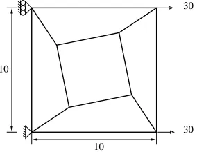
A patch test with five elements is performed with the Simo-Rifai enhanced as-sumed strain quadrilateral [22]. Figure 4.1 shows the set up. Minimal number of boundary conditions are used and the material properties and initial geometry remain constant during loading (linear). The element should have the ability to
10 10
30
30
Figure 4.1: patch test setup
produce constant stresses. Due to the addition of a strain field which in the end is used to compute the stresses it is not trivial a constant stress is obtained over the element. The transformation performed at the element its center should guarantee this. Changing the node numbering (frame invariance) should have no influence on the outcomes. This can also be checked with this test setup. The EAS strain matrix ˘Ben generates the same functions in each direction for the strain vector. By swapping terms of equation 4.2, the element has still the same properties in ξ and η direction.
4.3. SIMULATIONS 23
4.3.3
Mesh distortion
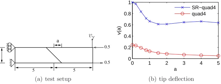
The Simo-Rifai quadrilateral is tested for it’s capabilities to avoid shear locking and insensitivity to mesh distortion. Figure 4.2(a) shows the test set up. The two only necessary constants for linear elasticity; E = 75 and ν = 0. The book of Zienkiewicz [22] shows the results of the test in Chapter 11. With the implemen-tation of the SR-quad inFeaTure the same results should be obtained.
As explained previously, the enhanced strain matrix supplies two parameters to enhance the normal strain and two parameters to reduce the shear strain. The exact linear solution of the problem is 1.
0.5
0.5 2
5 5
a vy
(a) test setup
0 1 2 3 4 5 0
0.2 0.4 0.6 0.8 1
a
v(a)
SR−quad4 quad4
(b) tip deflection
Figure 4.2: mesh distortion sensitivity
The SR element is compared with a normal quad4 element. Figure 4.2(b) shows that the EAS element performs overall much better than the quad4 element which suffers severely from shear locking. The SR quad seems relatively insensitive to mesh distortion. For the last valuea= 5 the element has a triangular form but only remains 0.363 away from the exact solution. These two properties, insensitivity to mesh distortion and creating an exact bending distribution are very useful when simulating sheet deformation processes.
4.3.4
Cook’s membrane
linear
24 CHAPTER 4. SIMO-RIFAI QUADRILATERAL
in the displayed case 4×4.
E = 70
F = 100
Figure 4.4 shows the results for the various combinations. The vertical
displace-F
44 16
48
vy
Figure 4.3: test setup with 4×4 mesh
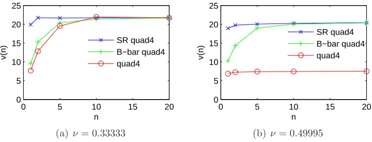
ment of the most upper-right node is displayed on the vertical axis. First, figure
0 5 10 15 20 0
10 20 30
n
v(n) SR−quad4
quad4
(a) ν= 0.33333
0 5 10 15 20 0
10 20 30
n
v(n)
SR−quad4 quad4
(b)ν = 0.49995
Figure 4.4: Cook’s membrane problem (linear plane strain)
4.3. SIMULATIONS 25
This effect reduces when the number of elements increase and thus the element shapes become less trapezoidal.
The good performance of the SR-quad is continued in figure 4.4(b). The en-hanced strain field gives 2 extra degrees of freedom to satisfy the implicit in-compressibility constraints at the integration points. The quad4 is locked by the volumetric constraints, the element is completely unusable in this setting.
Geometric non-linear
The same test as above is now evaluated geometrically non-linear. The total load of 100 Newton is applied in 5 steps. Enough accuracy is obtained at an internal force unbalance ratio of 10−3. Goal is, beside checking the functioning of the element in
an incremental-iterative setting, to compare the computational efficiency. A quad4 modified with the B-bar method is added. This element is adapted to function properly in the incompressible situation by underintegration of the volumetric part of the B-matrix. Figure 4.5(a) is very similar to figure 4.4(a), only displaying an
0 5 10 15 20
Figure 4.5: Cook’s membrane problem (non-linear plane strain)
even better convergence of the SR-quad. The overall displacement of the tip node has decreased due to the stiffening behavior of the geometry.
The B-bar element shows its purpose in 4.5(b), though still being less effective than the SR-quad. The quad4 is identical to the previous, linear, situation.
26 CHAPTER 4. SIMO-RIFAI QUADRILATERAL
4.3.5
Bending process
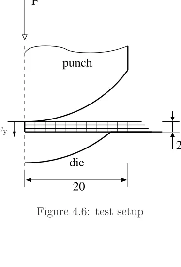
To show the EAS element’s capabilities in sheet deformation processes a model was reached by Corus, IJmuiden. The model represents the bending process of a plate. The plane strain assumption will simplify the problem to 2d. In Figure 4.6 the process is shown. The simulation is performed with various mesh sizes as seen in Table 4.1. The used geometry and the material model is in Appendix B.
The total displacement of the punch is four millimeter in negative vertical direction. The simulation is divided in 80 steps. 5 steps of the 80 steps are used to simulate springback of the plate.
20
punch
die
F
2
vyFigure 4.6: test setup
Table 4.1: mesh sizes
number of elements mesh size
500 10x50
125 5x25
60 3x20
30 3x10
4.3. SIMULATIONS 27
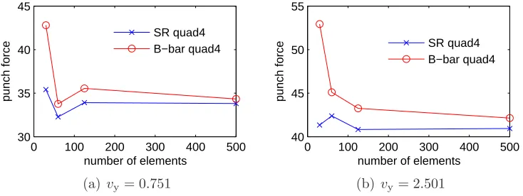
elements. The SR-quads are converging more rapidly to the final solution, even the very coarse meshes are reasonably in the range of the expected solution.
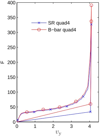
At Figure 4.8 the load curves are displayed for the two elements. The used model for this plot is the 3x20 mesh. The SR-quad reacts less stiff overall. Es-pecially the moment where the plate has contact with the punch and the die at all places along its boundaries, there is a large difference at pressing forces. When the punch is moved upwards a little, there is also a big difference.
State variables at the end of the total process, like the equivalent plastic strain or Von-Mises stress, are almost indifferent with respect to the element used. The cause of this is that the simulation is displacement driven (displacements are pre-scribed). In this case the main benefit of the EAS based elements is the more accurate prediction of the punch force. If the problem were to be force driven, results should be different. In this case the SR-quad should prove its value like it did in the linear tests.
Decreasing the mesh any further, for instance 1x10, did not give proper results. First problem can be that the geometry can not be modeled sufficiently, especially with respect to the contact elements. Secondly, in plasticity problems, constitutive properties are in general high order functions of the coordinates within the element. Sampling these functions only at two integration points along the total thickness of the plate might not be enough. A version with extended integration scheme along thickness might solve this problem. The subspace of the constraints will not get a higher rank by adding more integration points than the normal 2x2 integration. A 2x10 mesh with extended integrated elements could be accurate and computationally efficient.
Figure 4.7: punch force at two steps
28 CHAPTER 4. SIMO-RIFAI QUADRILATERAL
0 1 2 3 4 0
50 100 150 200 250 300 350 400
F
SR quad4 B−bar quad4
vy
Figure 4.8: loadcurve
element. As seen in Figure 4.3.3 the element behaves remarkable when distortion levels increase. The extra computational effort that has to be done for the SR quad4 is 34% in comparison with the B-bar quad4 for the 500 element mesh.
Table 4.2: computational results of 500 element mesh
elapsed time number of element in seconds iterations
SR quad4 25.1 274
B-bar quad4 18.7 221
4.4
Conclusions
4.4. CONCLUSIONS 29
Table 4.3: computational results of 125 element mesh
elapsed time number of element in seconds iterations
SR quad4 7.82 254
B-bar quad4 6.36 221
Seen from the computational perspective, the extra work needed to be done seems little whereas the improvements can be large. There are no problems with stability as would appear with reduced integrated elements. The convergence of the enhanced element in non-linearity has decreased a bit compared to the displacement based element.
Chapter 5
‘RESS’ 3d solid-shell
5.1
Introduction
In this chapter the RESS element as proposed by Sousa and co-authors is treated [14, 15, 16]. The abbreviation RESS stands for Reduced integration, Eas, Solid-Shell. These methods make a ‘standard’ 3d element suited for thin walled analysis. In first instance a reduced integration scheme is adopted to alleviate both volumet-ric and shear locking. Due to the reduced integration, a stabilization procedure has to be initialized to prevent hourglass modes. Secondly the strain in thickness direction is enhanced to counter thickness locking and the volumetric locking that could not be cleared completely by the RI procedure. Finally, in the stabilization procedure, the out-of-plane shear strains are set to zero and the volumetric part is deleted by using a B-bar procedure.
The element is programmed inC++ with aid of the FeaTure toolbox. The
toolbox includes algorithms for solving non-linear problems. This chapter is treat-ing all formulations for the geometric non-linear case.
5.2
Formulation
5.2.1
Introduction
When solving non-linear problems a clear distinction has to be made between iterations and increments. An increment is a predefined load or displacement step. For instance a load can be divided in various steps solved per increment. An iteration is an attempt to obtain a converged increment.
There are two distinctive configurations for a geometric non-linear problem: the reference configuration, and the current configuration. In total Lagrange pro-cedures the reference configuration remains the undeformed starting configuration, even after certain increments. The updated Lagrange method sets the
32 CHAPTER 5. ‘RESS’ 3D SOLID-SHELL
tion of the last converged increment as the reference configuration. So with a total Lagrangian procedure, integrals remain over the starting geometry. States have to be described in that geometry, hence the use of the 2nd Piola-Kirchhoff stress tensor and the Green-Lagrange strain tensor. Within an updated procedure the reference geometry is not far away (only one increment) from the sought solution. Therefore if increments remain small, linear state variables can be used, Cauchy stress and the linear strain tensor. Drawback is that between increments previous stresses have to be rotated to the new geometry.
The approach for the RESS element could be best described as a mixed ap-proach. The reference configuration is updated to the last converged increment. Within an increment non-linear states are used to make a new converged incre-ment. So the states and integrals within various iterations remain functions of the reference configuration.
5.2.2
EAS implementation
The implementation of the EAS method in (geometric) non-linearity is almost identical to the linear case. The potential energy form is very similar compared to Equation 3.34 for linearity. This form for non-linearity is known by the name of Veubeke Hu-Washizu. The proceeding formulations use the prefixed variable ias an iterative counter and a prefixed nas an incremental counter.
ΠVHW(u,E,S) = ΠVHWint −ΠVHWext (5.1)
E(u) is the Green-Lagrange strain.
E(u) = 1 2 ¡
FTF−1¢ (5.4)
The strains are enhanced similarly as Equation 3.42. The second term of ΠVHWint is discarded with the orthogonality condition. As result of the variation of the remaining part of potential energy toα and u two internal force vectors have to be taken into account:
fuint=
The external force vector is the same as was for the linear case:
5.2. FORMULATION 33
The resulting system of equations will become:
·
The vector i+1iu˜ is an attempt to make equilibrium within an increment. The static condensation procedure is invoked to discard i+1iα.
¡
Klg+Knlg−GTA−1G¢ i+1iu˜ =fuext−fuint+GTA−1fenint (5.9) The displacement based stiffness matrix is split into a geometric stiffness part Klg and a stress stiffening part Knlg. Matrices Aand Gare according Equation 3.48, only using differently formulated B-matrices.
5.2.3
Coordinate systems
Whenever expressing tensors in numbers, except a zeroth order tensor, coordinate systems have to be specified in which the tensor components are pointing. The RESS element is formulated with the aid of three different coordinate systems. These are, a global cartesian coordinate system, an orthonormal coordinate system and a convective coordinate system based on the natural coordinates. The three systems are shown in Figure 5.1 and listed in Table 5.1. The orthonormal and the natural system are expressed as a set of vectors in the cartesian system. The basis is defined with three base vectors. The assignation global means equal for
6
Figure 5.1: various coordinate systems
34 CHAPTER 5. ‘RESS’ 3D SOLID-SHELL
Table 5.1: various coordinate systems
coordinate system base vectors coordinates environment symbol orthonormal r1,r2,r3 p,q,r local ˆ
Below the definition of the natural coordinate system is given. Note that these are the covariant base vectors.
£
The orthonormal system is constructed at the element’s center. All partial deriva-tives used to build the system are therefore evaluated at (ξ, η, ζ) = (0,0,0). The system is constructed once with the undeformed geometry and is updated after-wards.
The system is orthogonal but not orthonormal, therefore:
ri = 1
ksi k
si i= 1,2,3 (5.17)
5.2. FORMULATION 35
elements so the quantities mentioned can be summed up easily. The orthonormal system is used for the constitutive computation. The advantage is that shell like structures can be modeled with for instance anisotropic properties in in-plane and thickness direction. Local stress and strain tensors are also beneficial in an incre-mental procedure since previous strains or stresses can be added without further transformations. If the tensor components were in global coordinates the proper-ties had to be rotated between increments. The natural coordinate system is used to create the strain-displacement- and the enhanced strain matrices.
5.2.4
Coordinate transformation
The Green-Lagrange strain tensor components are formulated in the directions of contravariant base vectors of the natural coordinate system.
n+1
The constitutive computation is in the orthonormal system. Therefore a transfor-mation has to be adopted. In matrix- vector notation.
ˆ
E=FE˘ (5.20)
Fis the operator which transforms tensor components from the natural convective coordinate system (gi), to the local orthonormal system (ri).
F=
The components of T needed to buildF are derived below. The transformation of the base vectors of the tensor can be written as:
36 CHAPTER 5. ‘RESS’ 3D SOLID-SHELL
Appendix A gives more details on coordinate transformations in general. The transformation can be expressed in matrix form.
T=
The first part of Equation 5.24 can be obtained by considering:
∂ xi ∂pj
ei =rj (5.25)
Which is in matrix form:
The second part of Equation 5.24 is simply the inverse of the Jacobian. So in total:
With this transformation the strain-displacement ˘B- matrices belonging to ˘E can be projected on the orthonormal system.
ˆ
B=FB˘ (5.29)
5.2.5
Enhanced strain parametrization
5.2. FORMULATION 37
The enhanced strains are defined in the directions of the natural coordinate system and thus have to be projected to the local orthonormal system with the coordinate transformation described in Section 5.2.4.
ˆ
Ben=F0B˘en (5.31)
where:
F0=F(ξ,η,ζ)=(0,0,0) (5.32)
The projection is equivalent to the one proposed by Simo and Rifai, [19]. Very ben-eficial about the enhanced strain parametrization is that with only one parameter both the volume- and the thickness locking phenomena can be countered.
5.2.6
Reduced integration
The normal full integration of a 3d hexahedral is 2x2x2. To counter volumetric and shear locking a reduced integration scheme is used. This scheme is 1x1 in in-plane direction and an unspecified number of integration points along thickness direction (1x1x5 for instance).
The main idea of multiple integration points along thickness is to model the complex constitutive behavior in plasticity. Note that the multiple integration points in thickness direction will not expand the subspace of the locking constraints any further than the 1x1x2 integration would do.
It is beneficial to choose an uneven number of integration points. This will make sure there is always an integration point at the center of the element which will ease certain computational procedures, for instance the stabilization procedure or updating the orthonormal system.
By using this integration scheme all terms of the ˘B-matrix which are constant or a function of ζ will be retained. The strain in the element consists of the following components:
˘
B= ˘B(c, ξ, η, ζ, ξη, ξζ, ηζ) (5.33)
The integration scheme samples at ξ, η = 0,0 and various values of ζ depending on the number of integration points chosen. This will reduce the strain matrix.
˘
B= ˘B(c, ξ, η, ζ, ξη, ξζ, ηζ) (5.34)
= ˘B(c,0,0, ζ,0,0,0) (5.35)
This strain matrix can be written out as a set of coefficients.
˘
B= ˘B(c, ζ) (5.36)
38 CHAPTER 5. ‘RESS’ 3D SOLID-SHELL
To prevent hourglass modes which correspond with these ‘lost’ terms, a stabiliza-tion procedure has to be initialized in which these terms are added back into the stiffness matrix and the internal force vector. These terms are:
˘
Bstab= ˘B(ξ, η, ξη, ξζ, ηζ) (5.38)
= ˘Bξξ+ ˘Bηη+ ˘Bξηξη+ ˘Bξζξζ+ ˘Bηζηζ (5.39)
Paragraph 5.2.8 treats the stabilization procedure.
5.2.7
Stiffness computation
The total stiffness matrix consists of a geometric stiffness part and a stress stiff-ening part. All integrals are calculated over the reference domain (last converged configuration). The geometry stiffness matrix can be computed as follows:
Klg= Z
Ω ˆ
BTDˆBˆdΩ (5.40)
The ˆD-matrix contains the components of the fourth order constitutive tensor in the local orthonormal coordinate system.
Klg=
This integral has to be worked out numerically. There is only one function ofζ in the ˆB so it can be programmed very efficiently. The needed ˘B- matrices can be found in Appendix C.
The stress stiffening matrix has to be calculated numerically.
Knlg = Z
Ω
( ˆBnlg)TSˆ9BˆnlgdΩ (5.43)
Due to the fact that Piola Kirchhoff stress acts in the last converged configuration, the integral should be over this domain. ˆBnlg is also derived at nx
ˆ
5.2. FORMULATION 39
The index k represents the node numbers of the element. The total number of columns of ˆBnlg will become 24. The notation used in the article by Sousa [15], is not proper since the base vectors r1,r2 and r3 are not functions of ξ norx. The orthonormal system is constructed at the center of the element and is therefore constant within the element. By using the set of coordinates p alongri the terms of ˆBnlgu can be constructed.
The derivatives of ξ top can be determined as follows.
The Knlg can now be calculated.
The internal force vectors are also calculated in the local orthonormal coordi-nate system:
40 CHAPTER 5. ‘RESS’ 3D SOLID-SHELL
scheme the following strain terms were lost:
˘
Bstab= ˘Bξξ+ ˘Bηη+ ˘Bξηξη+ ˘Bξζξζ+ ˘Bηζηζ (5.52)
The stabilization stiffness matrices corresponding with the ˘B-matrices:
KHG =Kξ+Kη +Kξη+Kξζ+Kηζ (5.53)
The strains are formulated in the natural coordinate system and have to be trans-formed to the orthonormal system to make the needed ˆB- matrices. The F0 is build at the element’s center.
ˆ
Bstab=F0B˘stab (5.54)
The sub-terms of the stabilization stiffness matrix are calculated as follows:
Kξ=
The term j0 is determinant of the Jacobi matrix evaluated at ξ = 0. Using the ‘total’ Jacobi determinant would introduce functions of ξ, making analytical integration more troublesome as will show later on. Note that all other possible cross products of the B-matrices will yield zero within the integral. For instance:
Z
The stiffness terms of Equation 5.59can be worked out efficiently by considering:
5.2. FORMULATION 41
All stabilization stiffness terms can be calculated analytically, no numerical inte-gration has to be performed.
Due to the integration scheme, the standard internal force vector fails to show nodal forces at the hourglass modes. The incremental stabilization internal force vector is defined as:
n+1
The necessary stresses may only be a function of the specified coordinates. If not, cross terms will not cancel out. Therefore the actual stresses can not be used, but are defined as:
The ˆB-matrices used for the internal force vector are evaluated at half of the increment.
All integrals above can be calculated analytically if the ˆD-matrix is assumed to be constant over the domain. Easy way out is to choose the constitutive model of the integration point in the middle. In the articles in which the RESS element is introduced, it is not clear what constitutive matrix should be used. In Article [15] a tangent material stiffness matrix is used. Second Article [16], uses only the elastic part of the material stiffness matrix for the stabilization procedure. The element as programmed inC++ uses the tangent stiffness matrix. Main motivation is that
42 CHAPTER 5. ‘RESS’ 3D SOLID-SHELL
The calculated stabilization force vector is incremental and not total. All previous contributions to the vector have to be taken into account.
n+1fHG= nfHG+ n+1
nfHG (5.75)
To prevent shear locking in the element in bending situations the two out of plane shear strains in the stabilization procedure are set to zero.
˘
Bξζ= 0 (5.76)
˘
Bηζ = 0 (5.77)
This approach is standard for shells. Constant shear strains which were calculated in the normal stiffness matrix are not canceled out, but these constant shear strains are subordinate in thin walled applications.
To prevent the volume locking phenomena in the stabilization stiffness matrix and the force vector, the B-bar method is used. The method assumes that the ˆB
consists of a deviatoric part and a volumetric part which is only evaluated at the element’s center.
ˆ
B(ξ) = ˆBdev(ξ) + ˆBvol(0) (5.78)
Since no constant terms are in the ˆB-matrices as used for the stabilization proce-dure, the volumetric part at the center will be zero. Therefore:
ˆ
Bvol(0) =0 (5.79) ˆ
B(ξ) = ˆBdev(ξ) (5.80)
The total system of equations will become:
¡
Klg+Knlg−GTA−1G+KHG ¢ i+1
iu˜ =fuext−fuint+A−1GTfenint−fHG (5.81)
5.2.9
Incremental procedure
Below follows a summary of the incremental procedures for the RESS element in a FEM program.
1. Compute Klg,Knlg, KHG and the EAS contribution −GTA−1G at n+1x. Sum the contributions and calculate the iterative displacements i+1iu˜ with the force vectorfuext−fuint+A−1GTfint
en−fHG. The incremental displacements n+1
nu˜ are the sum of all previous iterative displacements i+1iu˜.
5.2. FORMULATION 43
Use the deformation gradient to update the local orthonormal system. The local orthonormal system should be rotated and therefore the stretching part of the deformation gradient needs to be disposed.
n+1
Calculate the strains over the attempt to reach the converged increment with halfway geometry and orthonormal system.
i+1
iα=−A−1Gi+1iu˜ (5.88) n+1
nEˆ = n+1/2Bˆ n+1nu˜+ n+1/2Bˆenn+1nα (5.89)
Note that the strain is calculated with the ˆB-matrices and not according 5.4. The calculated strain is linearized over the increment. The ˆB matrices are calculated as follows:
n+1/2Bˆ = n+1/2FnB˘ (5.90)
n+1/2Bˆ
en= n+1/2F0nB˘en (5.91)
Note that the F-matrix is not the deformation gradient but the convective to local operator (5.21). The strain n+1nEˆ is used to calculate the stress with a constitutive model. This stress is used for calculation of the internal force vectors, but not the stabilization force vector.
3. determine the internal force vectors, fuint, fenint, fHG. The stabilization force vector is the previous force vector plus the new attempt, according Equation 5.75.
4. check if required accuracy in the force vector is obtained.
(a) No. Start from the top by building new stiffness matrices (in case of full Newton-Rhapson procedure).
(b) Yes. Make the current geometry the reference geometry for the new increment.
nx= n+1x (5.92)
n£
r1 r2 r3 ¤= n+1£ r1 r2 r3 ¤ (5.93)
44 CHAPTER 5. ‘RESS’ 3D SOLID-SHELL
In the article of Sousa and co-authors [15] several formulations are very pecu-liar. Especially the notations of the iterative-incremental procedure is question-able.
• First of all, the prefix n+1n, seems to be used for both iterative and incre-mental steps in the solving process. Equation (41) of Article [15] on page 170 shows n+1nd as an iterative change of the displacement. The equations as depicted in “Box 3. Computation of trial elastic stress” on page 170 seem to take n+1ndas an incremental change of the displacement.
• As derived in Section 3.5, theα-vector should be determined per iteration, exactly similar asuis determined per iteration (by means of a linearization step). The static condensation procedure should follow procedures described by Equation 3.71.
• The first equation of the “Box 3. Computation of trial elastic stress” in Article [15] does not include the effect of the internal force vector on theα -vector. Writing out the static condensation procedure will give:
i+1
iα=−iA−1 iGi+1iu˜− iA−1ifenint (5.94) The simplification of leaving the internal enhanced force vector out of the equation as made in the article is not explained. References as cited in the article, do not give the justification.
• The element is implemented in C++ according the article. The internal
enhanced force vector is not taken into account for calculation of α. The results of the non-linear tests as displayed in Section 5.3, are despite the formulations, showing that the element as implemented seems to function properly.
5.3
Simulations
5.3.1
Introduction
Several simulations are carried out to investigate the functioning of the element. The element is programmed inFeaTure. This package does not contain contact
elements which can be necessary to simulate forming processes. Therefore tests have to be made in which no ‘active’ contact between objects occurs.
The first test performed is to check the functioning of the element in linearity. The test of the deflection of a clamped square plate was introduced by Sousa [14] in the same article in which RESS is proposed. Results of the article can be easily compared with self-made results obtained by the RESS element as implemented
5.3. SIMULATIONS 45
element purely based on the EAS method, the HCIS12 element is programmed [5, 11]. The element is of the same authors as the RESS element.
The second test is the stretching of a cube and has as goal to check wether the incremental-iterative procedure works properly and the calculated strains are accurate.
The third test is the bending of a strip. This should show the purpose of the element: good thin walled behavior in bending situations. The problem is highly geometrically non-linear.
For all tests, the integration scheme of RESS is set to 1x1x5.
5.3.2
Clamped square plate
First test with the element is in the linear range, both geometrically and constitu-tive. In the article by Sousa [14] it is introduced. Figure 5.2 shows the test set up. Due to symmetry only a quarter of the plate has to be modeled. The 2x2 mesh is displayed in the figure. The edge of the plate is completely clamped. The needed constants:
L= 100
E= 10000 F = 16.367
Three elements are used for comparison, a linear 8 node hexahedral (HEX8), a quadratic 20 node hexahedral (HEX20), and a linear 8 node hexahedral which is modified with the EAS method (HCIS12). The HCIS12 uses 12 internal EAS parameters to make the element suited for shell analysis [5, 11]. The HEX8 and the HEX20 element use 2x2x2 integration. The test is performed four times in
L t
F
46 CHAPTER 5. ‘RESS’ 3D SOLID-SHELL
total. Two times with ν = 0.3 and ν = 0.499 and two times with t = 1 and t= 0.1. The normalized deflections of the center node are displayed in Figure 5.3. On the horizontal axis the number of elements along the sides of the modeled part are displayed. Visible is that the standard linear hexagonal element is completely useless in most cases. The quadratic version shows good performance when the aspect ratio is low. If the incompressibility constraint is enforced and the aspect ratios become larger, the accuracy of HEX20 becomes less. The HCIS12 element and the RESS element show very good behavior in all situations. The RESS element performs the best. Even in the situation where t = 0.1, the enhanced elements perform very well. The aspect ratio in this case is 250 which are shell like dimensions.
The results for the RESS element are exactly the same as the ones found by Sousa, showing that the element performs as intended.
2 4 6 8
Figure 5.3: normalized displacements
5.3. SIMULATIONS 47
Table 5.2: computation times of 8x8 mesh, ν = 0.3 and t= 1
element time in seconds
HEX8 0.187
HEX20 7.462
HCIS12 0.279
RESS 0.242
As expected, the HEX20 element is the most computational inefficient. The number of (external) degrees of freedom per element are 36 more in comparison with the HEX8 element, resulting in considerably larger stiffness matrices. The HCIS12 element has 12 (internal) degrees of freedom more then the HEX8 element but remains computational efficient. The RESS element performs a bit better than the HCIS12 element. Expected is that RESS should be considerably more efficient than HCIS12 [14]. Optimizing the C++ code for fast computation, or compiling
the program for speed should show more differences between RESS and HCIS12.
5.3.3
Cube stretching
5
3 7
8 z
1 4 y
2
x 6
Figure 5.4: test set-up
48 CHAPTER 5. ‘RESS’ 3D SOLID-SHELL
The solution of this problem can be found exactly by solving a differential equation.
K = ∂ F ∂u =
EA L0+u
F =EA(ln(L0+u)−ln(L0))
eEAF = L0+u
L0 The following parameters were used:
L0= 2
A= 4
F = 840000
The exact solution of the problem is u = 3.436563657. With a coarse number
100 101 102 103 3
3.5 4 4.5
number of increments
u
ress exact
Figure 5.5: displacement versus nr. of increments
of increments the displacement is overestimated. This is because