R E S E A R C H
Open Access
An enhanced weighted performance-based
handover parameter optimization algorithm for
LTE networks
Irina Mihaela B
ă
lan
1*, Bart Sas
2, Thomas Jansen
3, Ingrid Moerman
1, Kathleen Spaey
2and Piet Demeester
1Abstract
This article introduces an enhanced version of previously developed self-optimizing algorithm that controls the handover (HO) parameters of a long-term evolution base station in order to diminish and prevent the negative effects that can be introduced by HO (radio link failures, HO failures and ping-pong HOs) and thus improve the overall network performance. The default algorithm selects the best hysteresis and time-to-trigger combination based on the current network status. The enhancement proposed here aims to maximize the gain provided by the algorithm by improving its convergence time. The effects of this enhancement have been studied in a rural scenario setting and compared to the original algorithm; the results show a clear improvement, faster convergence, and better network performance, because of the enhancement.
Keywords:LTE, Self-Organization, handover, operator policy, PDP
1 Introduction
As the demand for services that can keep pace with the needs of the mobile client is increasing, mobile network operators have to look for new solutions for providing their services faster and better than ever before. The promise of auto-tunable functions that control different network mechanisms, such as handover (HO), load bal-ancing, and admission control, is slowly becoming a very tempting reality, for both operators and vendors. The self-optimization of future radio access networks is one of the main topics of today’s research [1,2].
HO is the core procedure in any mobile network as it guarantees users’freedom of movement while still being provided high quality services. User satisfaction is directly linked to the success rate of this procedure as well as its being as seamless as possible. In the currently deployed networks, the control parameters that govern HO are set to static values, and their updates are done on a long timescale (days and weeks), as part of maintenance operations or in response to an emergency situation. This approach is both time and effort consuming, and it
might not be carried out as often as necessary, resulting in sub-optimal network performance.
The benefits of self-organizing networks (SONs) have been proven by several studies in recent years. Similar studies in this field [3-5] usually attempt to minimize only one of the HO performance indicators (HPIs), such as Radio Link Failures (RLFs), HO ping-pongs (HPPs) or HO failures (HOFs), in an effort of improving network performance. However, since the relationships between these HPIs is a very close one, they should be considered as a whole when trying to optimize HO performance. A control parameter setting that, for example, diminishes the occurrence of ping-pong HOs will also most likely increase the number of RLFs. User mobility history has also to be used to predict future possible HOs and choose the best HO target cell [6]. As expected, the L3 filtering coefficient of the measurements of the strength of the cells around the user also has an impact on the HO performance [7]. The present study detailed in this article is a continuation of the studies previously pre-sented in [8-10]. The aim of the default Weighted Perfor-mance based HO Parameter Optimization algorithm (WPHPO) described in these articles is to dynamically modify the settings of the control parameters according to the current network performance situation, as opposed
* Correspondence: [email protected]
1
Department of Information Technology (INTEC), Ghent University - IBBT, Gaston Crommenlaan 8 Bus 201, 9050 Ghent, Belgium
Full list of author information is available at the end of the article
to them being set to fixed values at all times. The main challenges facing this algorithm is finding the perfect balance between deriving the proper parameter settings of the HO process in a short amount of time and ensur-ing that the network is in a stable operatensur-ing point for a long time afterwards. The strength of this algorithm and its enhancement resides in the fact that no new measure-ments, interfaces, events or signalling need to be added to the already standardized ones, which is to be consid-ered by any operator or vendor that would implement this approach. A drawback of the default algorithm is that it is too sensitive to changes in performance, which determines a slow convergence. This problem is targeted by the enhancement presented in this article.
The rest of this article is structured as follows. In Section 2, the main input measurements, control parameters and assessment criteria of the algorithm are presented. An enhancement approach is proposed in Section 3. A short sensitivity analysis is depicted in Section 4. Section 5 pre-sents the simulator tool and the investigated scenarios. The comparative simulation results of both the default algorithm and the enhanced version are included in Sec-tion 6. Conclusions and an outlook on future studies are given in Section 7.
2 Weighted performance based HO parameter optimization algorithm: a quick primer
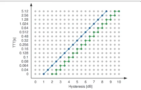
The weighted performance-based HO parameter optimi-zation algorithm (WPHPO) has been previously described in [8-10]. The network is constantly being monitored and input measurements (see Section 2.1) and certain perfor-mance metrics (see Section 2.2) are collected. Based on this input information, for each observation interval (referred to as a SON interval), the WPHPO calculates an overall performance metric (see Equation 1) and compares it with its previous value. Then, the algorithm will attempt to find a new pair of HO control parameter settings (also called HO operating point-HOP-Section 2.3) following a diagonal line through the HOP possible value space. Given the current HOP, the WPHPO will go up or down on the corresponding diagonal and pick the next HOP. This can happen by changing both values in a single step (blue line in Figure 1) or only one per step (green line in the same figure).
2.1 Input measurements 2.1.1 RSRP
The 3GPP specifications [11] define Reference Signal Received Power (RSRP) as input measurement for the HO algorithm. RSRP is defined as the linear average over the power contributions (in W) of the resource elements that carry cell-specific reference signals within the con-sidered measurement frequency bandwidth. The RSRP is measured for the current serving eNB (SeNB) as well as
for other eNBs in the user’s vicinity. It is used for ranking the different cells as input for HO and cell reselection decisions.
2.1.2 SINR
The signal-to-interference noise ratio is derived from the RSRP value of the SeNB and the RSRPs of all the other eNBs in the scenario plus thermal noise. If radio condi-tions worsen to the point where data can no longer be sent to the user, a call will be dropped.
2.2 HO performance indicators (HPIs) 2.2.1 Radio link failure ratio
The radio link failure ratio (RLF) is the probability that an existing call is dropped before it was finished, if the user moves out of coverage (SINR< -10 dB for 1 s). It is calculated as the ratio of the number of RLFs to the num-ber of calls that were accepted by the network.
2.2.2 HO failure ratio
The HO failure ratio (HOF) is the ratio of the number of failed HOs to the number of HO attempts. The number of HO attempts is the sum of the number of successful and the number of failed HOs. A HO is considered to have failed when the user tries to connect to the Target eNodeB (TeNB) but fails because of poor radio condi-tions. The user will then try to handback to its Serving eNodeB (SeNB). If this also fails (user has already moved out of the coverage area of SeNB), then the user will be dropped. In other words, although HO failures are caused by poor DL conditions (similar to RLFs), they will not result in a RLF unless the handback to the SeNB also fails. However, handback failures are added to the RLFs when calculating the RLF ratio.
2.2.3 Ping-pong HO ratio
If a call is successfully handed over to a TeNB and then it is handed back to the SeNB in less than the a critical time (Tcrit= 5 s), then this HO is considered to be a ping-pong HO (HPP). The HPP ratio represents the number of HPPs divided by the total number of successful HOs. It is the extra signalling and the possible traffic loss ping-pong HOs introduce that make them unwanted events. LTE only supports hard HO so there will be a certain inter-ruption time associated with every HO, when the user will not be connected to any eNB.
2.2.4 HO performance (HP)
The HO performance is an operator policy-based weighted sum of the three metrics described above and offers an overall performance evaluation. The HP is cal-culated according to Equation 1.
HP =wRLF∗RLF +wHOF∗HOF +wHPP∗HPP
wRLF+wHOF+wHPP
(1)
minimized and which can be tolerated. Section 6 pre-sents the outcome of applying the (E)WPHPO with a combination of [wRLF= 2, wHOF = 1, wHPP = 0.5]; this will give priority to the reduction of RLFs, while HO failures are to be avoided but ping-pong HOs are just tolerated as inevitable side effects of the RLF reduction. The HP as calculated using Equation 1 will be a number between 0 and 1.0 represents perfect system perfor-mance, and 1, worst possible performance.
2.3 Control parameters 2.3.1 Hysteresis
The UE monitors its serving cell (SeNB) and neighbour eNBs around it (NeNBs) by periodically performing downlink radio channel measurements of the RSRP on the pilot channel. If certain network configured condi-tions are satisfied, then the UE sends the corresponding measurement report (MR) indicating the triggering event. In our case, the MR trigger is the condition A3 [12], a relative condition between cells. A HO is initiated when the following condition is met for a certain amount of time:
RSRPNeNB>RSRPSeNB+ Hys (2)
where RSRPNeNBand RSRPSeNBare the RSRP values of
the of a neighbour and of the current serving cell,
respectively. The valid hysteresis values varies between 0 and 10 dB with steps of 0.5 dB, resulting in 21 valid hys-teresis values.
2.3.2 Time-to-trigger
The time the RSRP condition in Equation 2 has to hold for initiating a HO is specified by the time-to-trigger parameter. The time-to-time-to-trigger values for LTE networks are specified by 3GPP (see [12, Section 6.3.5]). The values are (0, 0.04, 0.064, 0.08, 0.1, 0.128, 0.16, 0.256, 0.32, 0.48, 0.512, 0.64, 1.024, 1.280, 2.560 and 5.120) in seconds. These 16 values are the only valid time-to-trigger values.
3 Enhancement proposal
The WPHPO algorithm presented above switches the direction in which it looks for a new HOP if the HP of the current SON interval is larger (worse) than the one calcu-lated for the previous one. This may cause slow conver-gence, since a small number of events (like ping-pong HOs or HO failures) may determine the direction to be switched and return to a previous point. Convergence time is vital in a live network, since the algorithm should respond in a timely fashion to changes in radio conditions or should derive a stable HOP in a certain amount of time. If valuable HOP changes are wasted switching between two or three values, then convergence may never be reached or it might
come too late, since the triggering situation has yet again changed.
In order to improve convergence time, such situations should be avoided. An extra threshold is introduced, which will allow the direction to be switched only if
per-formance degrades with more thanx% compared to the
previous value. In the following, thisx% increase will be
referred to as Performance Degradation Percentage
(PDP). By tolerating worse performance, needless switch-ing of optimization direction due to isolated incidents is avoided. Also, this will mean that, in the same amount of time, the enhanced WPHPO (EWPHPO) will be able to derive a more suitable HOP, since valuable changes will not be wasted by ping-ponging between two HOPs.
The EWPHPO algorithm will operate as follows:
if(SON interval over) {
collect HPIs for the previous interval calculate HP weighted sum
if(current HP value is PDP% worse than previous
HP value)
switch optimization direction
else
maintain current optimization direction change current HOP
}
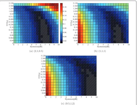
4 Sensitivity analysis
A sensitivity analysis that took into account all the 336 possible combinations of Hysteresis and TTT values was performed, and it motivated the decision of working on a diagonal line. A small HOP value will determine a low number of RLFs, while the HO failure and ping-pong HO ratios in this case will be high; the situation will be inversed for large HOP values. Since the biggest influence will be attributed to the RLFs (wRLF= 2), the‘
optimal-performance’ region will be placed somewhere in the
middle of the Hysteresis-TTT plane. Remember that the lower the value of the HP (e.g. less unwanted events), the better the performance.
As mentioned before, the values for the weights in Equation 1 are a direct translation of the operator policy. Thus, the operator of a mobile network can influence the performance of the (E)WPHPO algorithm by manipulat-ing the weight mix. Although any combination of weights can be applied to Equation 1, not all such combinations are actually logical or preferred. If, for example, all the weights are set to the same value (all the three statistics are given equal importance), the algorithm will attempt to level the number of RLF with that of the ping-pongs and the HO failures, although the latter happen very sel-dom. If the weight of the RLF is equal to the one of the ping-pongs, then this certainly will introduce oscillation of the HOP since, once the RLF ratio decreases, the
ping-pong ratio increases. Also, extreme values for one weight compared to the other two, will probably reduce HPI in question but will increase one of the other two well beyond the maximum accepted thresholds. The operator should take this into account and set some realistic per-formance targets, which will be reflected by the values of the weights.
An outcome of such a sensitivity analysis is presented in Figure 2 for a scenario with 2,500 users, moving at 50 km/h and generating a constant load. The position the optimal HOP is mainly determined by the scenario con-ditions (user mobility and load) and the weight mix.
The weight mix will have a direct impact on the HP values and thus on the optimization decisions. If RLFs are given the highest weight (see Figure 2(a)), the HOPs that offer the best performance will be located close to the cen-tre of the HOP space. If all statistics are given equal weights (see Figure 2(b)), then the optimal HOPs will shift towards higher value settings (since the algorithm will try to level them out and the number of ping-pong HOs is much bigger than that of the call drops). Finally, giving ping-pong HOs the highest weight (see Figure 2(c)) will shift the optimum even further to the right.
5 Simulator and scenarios
The results presented below have been obtained using a OPNET (http://www.opnet.com)-based simulator in a rural scenario. This simulator models eNBs, UEs, and the communication between eNBs. The main simulation parameters are given in Table 1. The simulation area
consists of 25 eNBs, placed on an equally spaced 5×5
grid. The distance between eNBs is given by the inter site distance (see Table 1). The users are initially distributed within the simulation area, and they start moving accord-ing to a random walk mobility model, all at the same speed. During the simulations, the UEs will alternate between an active (a call is ongoing) and an inactive state (idle state). After the user has been idle for an appropri-ate amount of time (drawn from an exponential distribu-tion), referred to as idle duration, it will start a call. The values of this mean determent the load of the network. The larger the mean of the distribution, the lower the load, as fewer users will simultaneously be active in the network. A user may only initiate one call at a time which can either be voice, video, or web. Voice calls have an average bit rate of 6.1 kbit/s (12.2 kbit/s with a 50% activity factor), while video calls have an average bit rate of 64 kbit/s, according to [13]. The user will go back into the idle state either when the current call finishes (in case of the web call, when all the data have been trans-mitted) or when this call is dropped (because of poor SINR conditions).
0 1 2 3 4 5 6 7 8 9 10 0
0.04 0.064 0.08 0.1 0.128 0.16 0.256 0.320 0.480 0.512 0.64 1.024 1.280 2.560 5.120
Hysteresis[dB]
TTT[s]
0.02 0.04 0.06 0.08 0.1 0.12 0.14 0.16 0.18
(a) (2,1,0.5)
0 1 2 3 4 5 6 7 8 9 10
0 0.04 0.064 0.08 0.1 0.128 0.16 0.256 0.320 0.480 0.512 0.64 1.024 1.280 2.560 5.120
Hysteresis[dB]
TTT[s]
(b) (1,1,1)
0 1 2 3 4 5 6 7 8 9 10
0 0.04 0.064 0.08 0.1 0.128 0.16 0.256 0.320 0.480 0.512 0.64 1.024 1.280 2.560 5.120
Hysteresis[dB]
TTT[s]
(c) (0.5,1,2)
Figure 2HP in HOP space for different weight combinations (wRLF,wHOF,wHPP).
Table 1 Simulation parameters
Parameter Value
Network layout 5×5 grid
Number of users 2,500
Inter-site distance (ISD) 1732 m
System bandwidth 5 MHz
Antenna type Omnidirectional
eNB Tx power 43 dBm
Pathloss model Okumura-Hata model for open space (according to [15]) Shadow fading deviation 5 dB (according to [14])
SON interval 3 min
RSRP Measurement interval 40 ms, L3 filtering over 200 ms (k= 10)
RLF detection T310= 1 s
Ping-pong HO detection timer 5 s
HP weight mix wRLF= 2,wHOF= 1,wHPP= 0.5
location of the user and correlated shadow fading a zero-mean Gaussian distribution in the log-domain with a standard deviation of 5 dB. Pathloss calculations are performed using the Okumura-Hata model for open space. Furthermore, shadow fading that is both auto-correlated in time and cross auto-correlated with the shadow fading of other antennas is considered [14], whereas fast fading is not considered. RSRP values for SeNB and NeNBs are computed every 40 ms and then filtered using Equation 3 as described in [12]:
Fn= (1−αRSRP)Fn−1+αRSRPMn (3) whereMn is the latest calculated RSRP value (layer 1
measurement); Fnis the updated, filtered RSRP value;
and Fn-1 is the previous filtered RSRP value. Thea in the previous formula is equal to 1/2k/4, wherek is the filtering coefficient mentioned in [7], and in this case will be 10. No layer 1 filtering is applied in the simula-tor, as layer 1 filtering is mainly used for filtering out fast fading, which is not considered in the simulator.
A RLF will be detected when the SINR of a call is under the minimum threshold (-10 dB) for a certain amount of time (1 s, similar value to the T310 timer [12]).
The 5 s timer for detecting a ping-pong HO is a simula-tor parameter. No value for this timer is given by the 3GPP specifications. This value was chosen to have the same magnitude as the T310 timer for the detection of RLFs.
The following scenarios were investigated by varying the speed of the users and the load being introduced in the system:
• Scenario 1: A constant speed and load scenario
where the user speed is 50 km/h and idle duration mean is 300 s.
• Scenario 2: Highway congestion scenario-during
the first hour of simulation, the speed changes from 120 to 3 km/h, and the load rises by modifying the mean idle duration from 300 s mean idle time to 0 s.
Note that the user speeds, ISD, pathloss and shadow fading characteristics have been chosen in such a way as to reflect the rural scenario.
6 Results
As part of initialization, all the eNBs in the scenario are set to have the same initial HOP. Subsequently, based on the observed performance, each cell will change its HOP accordingly and independently. Note that all the results presented in the tables are averaged over the entire simulation time (excluding the first 300 s which is the warm-up period) and all the eNBs in the scenario (unless stated otherwise). The HP is calculated using Equation 1. The results for the reference case (no SON
algorithm was enabled; the HOP was set to a fix value during the entire simulation time) were compared against those of the default WPHPO (PDP = 0%) and several values for the PDP of the EWPHPO.
6.1 Diagonal vs zigzag
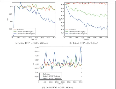
Initially, the two different possibilities of crossing the HOP space (diagonal and zigzag as shown in Figure 1) and the effects they would have on the performance of the network were considered. The two approaches were tested in scenario 1 for different starting HOPs: two extreme ones (10 dB, 5120 ms; and 0 dB, 0 ms) and a middle one which falls within the optimum performance region (4 dB, 480 ms). The results after one hour simu-lation time are presented in Figure 3 and Table 2.
Such extreme initial settings are not customary and should be avoided; however, they can occur in the net-work, being caused by various incidents or a series of incorrect setting propagating through the network. Also, the default WPHPO should be able to deal with any initial setting, no matter how extreme it is. It is especially in these extreme settings that the WPHPO should prove to be most useful in remediating the situation and bringing the HOP back to more acceptable setting.
When stating in an extreme HOP (such as (10 dBm, 5120 ms) or (0 dB, 0 ms)), the diagonal approach per-forms significantly better than the zigzag. This is because in this approach, both Hysteresis and TTT are changed in each step; thus, the performance variance between two consecutive HOPs is more significant, and the chances for ping-ponging between two of them will decrease. In these cases, the WPHPO improves performance in a short amount of time. The exception here is the (10 dB, 5,120 ms) with zigzag case, where the algorithm does not manage to converge in the given time frame (if more time were allocated, this approach too would improve performance; see Figure 4(a) in the next section), because of repeated changes between the same HOPs. This would be the exact situation which the PDP would help avoid.
On the other hand, when starting from an optimal HOP (4 dB, 480 ms), the diagonal is no longer the optimal choice. In this case, the high performance variance between two neighbouring HOPs constitutes a disadvan-tage. The zigzag provides higher granularity and thus gives better results when already in a optimum performance area. The operators may also favour the zigzagging approach since it enables the use of any HOP and provides more control.
6.2 Influence of PDP 6.2.1 Scenario 1
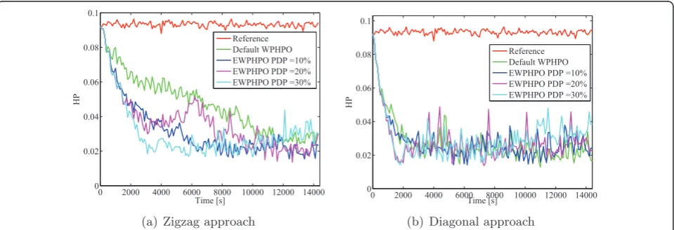
in which it optimizes the HOP. By introducing the PDP, increased convergence and performance when starting from an extreme HOP are targeted. A setting of PDP = 0% means that the default WPHPO is used. Results for high initial HOP settings (10 dB, 5,120 ms) for both zig-zag and diagonal use are shown in Figure 4 and Table 3. In case of the zigzagging, the introduction of the PDP
determines the most visible performance improvement. A setting of 30% is the overall best (see average in Table 3), while the 20% setting gives the best final value. When using the diagonal, the addition of the PDP also shows improvement with an ideal setting of 20%, in terms of rapid decrease in the first simulation hour and final values. Results for low initial settings (0 dB, 0 ms) are pre-sented in Figure 5 and Table 3. Similarly, the introduc-tion of the PDP speeds up convergence, only this time, in the case of the zigzag use, a 10% PDP gives best per-formance and insures the lowest final value for the HP.
This is because the initial performance (see ‘Default
WPHPO’ case), is converging much faster and has
started from a lower initial value.
6.2.2 Scenario 2
In this scenario, the initial HOP (8 dB, 160 ms) reflects a setting that would be appropriate for the initial state of the network. The decrease in speed and increase of load occur gradually during the first simulation hour. Results are depicted in Figure 6 and Table 3. In case of
Table 2 Diagonal vs. zigzag
Initial HOP SON approach RLF(%) HOF (%) HPP (%) HP
10 dB, 5120 ms Reference 35.48 0 0 0.20 WPHPO zigzag 35.99 0 0 0.20 WPHPO diagonal 27.76 0 2.35 0.16 0 dB, 0 ms Reference 0 0.04 67.82 0.097
WPHPO zigzag 0 0.01 52.78 0.075 WPHPO diagonal 0.09 0 33.62 0.048 4 dB, 480 ms Reference 0 0 13.79 0.019 WPHPO zigzag 0.35 0 12.96 0.020 WPHPO diagonal 1.27 0 11.66 0.023 0 500 1000 1500 2000 2500 3000 3500 0
0.05 0.1 0.15 0.2
Time [s]
HP
Reference
Default WPHPO zigzag Default WPHPO diagonal
(a) Initial HOP =(10dB, 5120ms)
0 500 1000 1500 2000 2500 3000 3500 0
0.01 0.02 0.03 0.04 0.05 0.06 0.07 0.08 0.09
Time [s]
HP
Reference
Default WPHPO zigzag Default WPHPO diagonal
(b) Initial HOP =(0dB, 0ms)
0 500 1000 1500 2000 2500 3000 3500 0
0.005 0.01 0.015 0.02 0.025 0.03 0.035 0.04
Time [s]
HP
Reference
Default WPHPO zigzag Default WPHPO diagonal
(c) Initial HOP =(4dB, 480ms)
0 2000 4000 6000 8000 10000 12000 14000 0
0.05 0.1 0.15 0.2
Time [s]
HP
Reference Default WPHPO EWPHPO PDP =10% EWPHPO PDP =20% EWPHPO PDP =30%
(a) Zigzag approach
0 2000 4000 6000 8000 10000 12000 14000
0 0.05 0.1 0.15 0.2
Time [s]
HP
Reference Default WPHPO EWPHPO PDP =10% EWPHPO PDP =20% EWPHPO PDP =30%
(b) Diagonal approach
Figure 4HP evolution with different PDP values with high initial HOP (10 dB, 5,120 ms) in scenario 1.
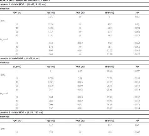
Table 3 HPIs values in Scenarios 1 and 2
Scenario 1 - initial HOP = (10 dB, 5,120 ms)
Reference
PDP (%) RLF (%) HOF (%) HPP (%) HP
- 33.37 0 0 0.19
Zigzag
0 22.64 0 4.97 0.13
10 14.96 0 6.03 0.094
20 13.94 0 6.34 0.088
30 11.31 0 5.62 0.072
Diagonal
0 9.59 0.002 9.38 0.068
10 6.40 0 9.61 0.050
20 4.99 0.001 12.02 0.045
30 6.08 0 11.21 0.050
Scenario 1- initial HOP = (0 dB, 0 ms)
Reference
PDP(%) RLF (%) HOF (%) HPP (%) HP
- 0 0.04 68.03 0.097
Zigzag
0 0.039 0.01 37.51 0.053
10 0.023 0.005 27.18 0.038
20 0.299 0.009 28.76 0.042
30 0.41 0.002 25.65 0.038
Diagonal
0 0.64 0.003 19.97 0.032
10 0.80 0.002 19.46 0.032
20 0.96 0.001 18.61 0.032
30 0.97 0.001 19.89 0.034
Scenario 2 - initial HOP = (8 dB, 160 ms)
Reference
PDP (%) RLF (%) HOF (%) HPP (%) HP
- 1.17 0 3.17 0.01
Zigzag
the reference (where no optimization in performed), the alignment of HOP setting, and thus of the performance, with the current network status happens much slower, after the changes have actually stopped. The (E)WPHPO reacts while the changes are ongoing. Since the algo-rithm starts in a HOP that is close to the optimum, the improvement due to the PDP is not so evident as before, but the performance is already very good (low HP). Nevertheless, a PDP of 20% is still slightly better as opposed to 0%, in both zigzag and diagonal cases.
The overall conclusion is that no matter whether the zigzag or diagonal is used, the addition of the PDP improves convergence time and performance. While dif-ferent scenarios and difdif-ferent initial HOPs might benefit from different settings of the PDP, a value of 20% has proven to be acceptable for all.
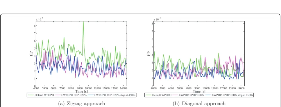
6.3 Disabling of EWPHPO
Once the EWPHPO manages to get the current HOP into a region that offers more stability and fewer oscilla-tions, it may be more beneficial to completely turn it off. This approach was investigated in Scenario 2, where the EWPHPO was switched off after 4,500 s. This time has been chosen based on the results in Figure 6, since after this time, the oscillations are significantly smaller than previous. The results are presented in Figure 7 and
Table 3. After the EWPHPO is turned off, the HOP remains fixed to the value it had at 4,500s. The oscilla-tions that appear in the blue curve are introduced only by fading, and strongly depend on the value of this HOP. Even thought this HOP belongs to the optimum performance region associated with the current load and speed, the variations in performance are still comparable to the case where optimization would still be enabled (pink and green curves). The average performance (mea-sured between 4,500 s and simulation end) with the EWPHPO disabled is slightly better than the enabled version (HP value 0.10 vs. 0.13 for the diagonal).
7 Conclusions and future study
In this article, an enhanced weighted performance HO parameter optimization (EWPHPO) is proposed, build-ing up on the studies previously presented in [8-10]. This algorithm will tune the Hysteresis and TTT of a LTE eNB, based on currently experienced performance. The enhancement consists in tolerating PDP% worse performance before switching the direction in which the algorithm is looking for the new HOP. The EWPHPO has been tested for two different scenarios with various initial HOPs.
The addition of the PDP speeds up convergence of the algorithm and thus improves system performance, in
Table 3 HPIs values in Scenarios 1 and 2(Continued)
10 0.59 0 2.49 0.006
20 0.51 0 2.75 0.006
20 stop at 4,500 s 0.53 0 2.87 0.007
Diagonal
0 0.40 0 3.58 0.007
10 0.41 0 3.97 0.007
20 0.38 0 4.01 0.008
20 stop at 4,500 s 0.33 0 3.96 0.007
0 2000 4000 6000 8000 10000 12000 14000
0 0.02 0.04 0.06 0.08 0.1
Time [s]
HP
Reference Default WPHPO EWPHPO PDP =10% EWPHPO PDP =20% EWPHPO PDP =30%
(a) Zigzag approach
0 2000 4000 6000 8000 10000 12000 14000
0 0.02 0.04 0.06 0.08 0.1
Time [s]
HP
Reference Default WPHPO EWPHPO PDP =10% EWPHPO PDP =20% EWPHPO PDP =30%
(b) Diagonal approach
both diagonal and zigzag approaches. As expected, the diagonal approach converges faster, while the zigzag offers better granularity. The EWPHPO works well when the initial HOP is an extreme value and manages to bring the HOP setting into a good-performance region in a short amount of time.
Once in the good-performance region, however, the EWPHPO performs less than optimal because of the constant change in HOP (every SON interval). The EWPHPO attempts to find an even better HOP, assum-ing that there is one. In this case, the zigzaggassum-ing approach performs better, since it only changes one of the two parameters (Hysteresis or TTT). Thus, it would be beneficial if the HOP would stop changing, once the variation in performance (in our case of the HP) would become significantly lower.
As a part of future study, the introduction of an auto-mated mechanism that would distinguish among types of performance variations, dividing the HOP space into
high and low performance variance regions (HPVR and LPVR) will be investigated. The PDP will be applied while the system is in the HPVR to speed up conver-gence towards the LPVR. Once the LPVR is reached, the EWPHPO will be disabled, and a fixed HOP will be selected. Of course, if the network conditions change and the high fluctuations in performance are observed, then the EWPHPO will again be enabled as the system moves into the HVPR.
Acknowledgements
The research leading to the above results has received funding from the European Union’s Seventh Framework Programme (FP7/2007-2013) under grant agreement no. 216284.
Author details
1Department of Information Technology (INTEC), Ghent University - IBBT,
Gaston Crommenlaan 8 Bus 201, 9050 Ghent, Belgium2IBBT-UA-PATS,
Middelheimlaan 1, B-2020 Antwerpen, Belgium3Technical University of Braunschweig, Braunschweig, Schleinitzstrasse 22, 38106 Braunschweig, Germany
0 2000 4000 6000 8000 10000 12000 14000
0
0 2000 4000 6000 8000 10000 12000 14000
0
Figure 6HP evolution with different PDP values using zigzag or diagonal approach with medium initial HOP (8 dB, 160 ms) in scenario 2.
4000 5000 6000 7000 8000 9000 10000 11000 12000 13000 140000 1
Default WPHPO EWPHPO PDP =20% EWPHPO PDP =20% stop at 4500s
(a) Zigzag approach
4000 5000 6000 7000 8000 9000 10000 11000 12000 13000 140000 1
Default WPHPO EWPHPO PDP =20% EWPHPO PDP =20% stop at 4500s
(b) Diagonal approach
Competing interests
The authors declare that they have no competing interests.
Received: 18 February 2011 Accepted: 17 September 2011 Published: 17 September 2011
References
1. 3GPP, Self-configuring and self-optimizing network use cases and solutions. Technical Report TR 36.902, http://www.3gpp.org
2. Next Generation Mobile Networks, Use Cases related to Self Organising Network, Overall Description, http://www.ngmn.org
3. D-W Lee, G-T Gil, D-H Kim, A cost-based adaptive handover hysteresis scheme to minimize the handover failure rate in 3GPP LTE system. EURASIP J Wirel Commun Netw2010, Article ID 750173, 7(2010)
4. A Schrder, H Lundqvist, G Nunzi, Distributed self-optimization of handover for the long term evolution, Self-Organizing Syst.534(3), 281–286 (2008) 5. J Alonso-Rubio, Self-optimization for handover oscillation control in LTE.
IEEE Network Oper Manag Symp (NOMS), (2010)
6. H Ge, X Wen, W Zheng, Z Lu, B Wang,A History-Based Handover Prediction for LTE Systems(CNMT, Wuhan, China, 2009), pp. 18–20
7. P Legg, G Hui, J Johansson, A simulation study of LTE intra-frequency handover performance, inVTC Fall. inProceedings 2010 IEEE 72nd Vehicular Technology Conference Fall,(Ottawa, ON, Canada), pp. 5–9 (2010) 8. T Jansen, I Balan, I Moerman, T Kürner, Handover parameter optimization in
LTE self-organizing networks, inIEEE 72nd Vehicular Technology Conference (VTC2010-Fall)(Ottawa, Canada, 2010)
9. T Jansen, I Balan, S Stefanski, I Moerman, T Kürner, Weighted performance based handover parameter optimization in LTE. Paper accepted to VTC Spring, Budapest, (2011)
10. I Balan, T Jansen, B Sas, I Moerman, T Kürner, Enhanced Weighted Performance Based Handover Optimization in LTE. (Paper accepted for Future Network and MobileSummit, Warsaw, 2011)
11. 3GPP TS 36.214 V8.2.0 (2008-03), Evolved Universal Terrestrial Radio Access (E-UTRA); Physical Layer-Measurements (Release 8).
12. 3GPP, Evolved Universal Terrestrial Radio Access (E-UTRA); Radio Resource Control (RRC); Protocol specification. Technical Report TR 36.331, section 5.3.11, http://www.3gpp.org
13. NGMN white paper, NGMN radio access performance evaluation methodology (January 2008)
14. R Fraile, JF Monserrat, J Gozlvez, N Cardona, Mobile radio bi-dimensional large scale fading modelling with site-to-site cross-correlation. Eur Trans Telecommun.19, 101–106 (2008). doi:10.1002/ett.1179
15. L Ahlin, J Zander, B Slimane, Principles of Wireless Communications. Studentlitteratur (2006). ISBN 91-44-03080-0
doi:10.1186/1687-1499-2011-98
Cite this article as:Bălanet al.:An enhanced weighted performance-based handover parameter optimization algorithm for LTE networks. EURASIP Journal on Wireless Communications and Networking20112011:98.
Submit your manuscript to a
journal and benefi t from:
7Convenient online submission
7Rigorous peer review
7Immediate publication on acceptance
7Open access: articles freely available online
7High visibility within the fi eld
7Retaining the copyright to your article