The daily variations of the vertical (Z) element of the geomagnetic field
around the coast of mainland Australia
R. J. Stening and T. Reztsova
School of Physics, University of New South Wales, Sydney 2052, Australia
(Received May 19, 2006; Revised January 22, 2007; Accepted February 27, 2007; Online published June 27, 2007)
Use is made of an array of magnetic stations spread across the Australian mainland to examine the daily variation of the vertical element Z of the magnetic field. On sections of the west and east coasts visual inspection of Z variations shows that they respond mainly to the onshore component of the horizontal field as predicted by Bennett and Lilley, though only south of about 22◦S on the east coast and south of 20◦S on the west coast. On the north and south coasts this “coast effect” is not clearly seen at periods corresponding to the daily variation, though it sometimes appears on shorter time scales. On the north and south coasts Z appears to be mainly controlled by the decrease with latitude of the overhead eastward ionospheric currents as measured by the latitude gradient in the northward field, X. By subtracting the vector Z variation at an inland station from Z at a coastal station, the anomalous coastal effect in Z is calculated at periods of 12 and 24 h. These data show that the coastal effect is not just related to the horizontal onshore component but that some phase change is also required. An increase with latitude of the overhead eastward currents is sometimes found in morning hours corresponding to the morning current system identified in earlier work.
Key words:Sq variations, coastal effect, induction, ionospheric currents.
1.
Introduction
The daily variations of the magnetic field observed on days free of magnetic disturbance or storms are thought to be due to a system of electric currents flowing in the iono-sphere, commonly known as the Sq system (Matsushita, 1967). Those who study this system usually use the hori-zontal northward (X) and eastward (Y) elements of the vari-ations of the field but avoid the use of the vertical (Z) field as it is often influenced by other effects. The Z field is most affected by different induced currents caused by conductiv-ity anomalies within the earth and by the proximconductiv-ity of a coastline.
Broadly speaking, the Z variation during times of mag-netic quiet has a peak around local noon in the southern hemisphere. This can be seen in the diagrams of Matsushita (1967) and arises mainly from the decrease with increasing latitude of the eastward currents in the ionosphere, includ-ing their reversal to westward beyond the focus of the Sq current system.
From August 1989 to June 1990 an array of 54 magne-tometers was running spread across the Australian main-land. This project was called the Australia-Wide Array of Geomagnetic Stations (AWAGS). Further information on the array may be found in Chamalaun and Barton (1993a, b). These data provide an unique opportunity to study the Z variation field in some detail. Please note that the emphasis of the present study is on times when no significant mag-netic disturbance is present so that the magmag-netic variations
Copyright cThe Society of Geomagnetism and Earth, Planetary and Space Sci-ences (SGEPSS); The Seismological Society of Japan; The Volcanological Society of Japan; The Geodetic Society of Japan; The Japanese Society for Planetary Sci-ences; TERRAPUB.
seen are mainly due to the Sq current system in the iono-sphere and the currents induced in the earth by the magnetic fields produced by that system.
Lilley and Parker (1976) showed that the vertical (Z) variation of the field on a magnetically quiet day (Kp≤1−) was consistently larger on the west coast compared to the rest of the continent, including the east coast. They further showed that the anomalous Z field at Gnangara, on the west coast, was best correlated with the onshore component of the eastward field YO.
Much of the earlier work on the geomagnetic coast effect, both observational and theoretical, has been reviewed by Parkinson and Jones (1979).
Also many of the investigations have concentrated on shorter period magnetic variations. For example Everett and Hyndman (1967) restricted their study to frequencies greater than 4 cycles per day. Goughet al.(1974) concen-trated on times during magnetic storms and periods from a half hour to several hours. Srivastavaet al. (2001) ex-amined both Sq ranges and substorm behaviour at Indian stations and found different behaviour of the Z component of Sq on the east and west coasts. This led them to postulate a region of lower conductivity in the east.
Bennett and Lilley (1973) obtained separate variations of amplitude and phase for 6,8,12 and 24-hour periods for the three magnetic elements over a magnetometer array in south-east Australia. They then identify a “normal” mag-netic variation at a magmag-netic station distant from the coast and vectorially subtract this from the variations at all sta-tions to obtain an anomalous variation, ZA, in the case of the
vertical component. They suggest that the best correlation for ZAagain occurs with the onshore component YOof the
110 115 120 125 130 135 140 145 150 155
Current Function External Component @ 02.00 GMT for 89/12/8 thru 89/12/9
Fig. 1. Map showing the location of observing stations. The vectors correspond to the magnetic field at 2 h UT on 9 December 1989, rotated clockwise through 90◦. A vector length equivalent to 5◦of longitude on the abscissa scale is equivalent to 28.5 nT.
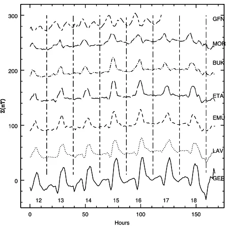
Fig. 2. Z variations at a chain of stations from the west coast at the bottom (GER) to the east coast at the top (GFN) during a fairly quiet magnetic period from 12 to 18 May 1990.
horizontal field variation. We shall seek to test this correla-tion with a larger number of stacorrela-tions around the Australian coast. Bennett and Lilley suggest that this effect might be explained by “lateral conductivity contrasts between ocean and land”. After examining various possibilities, Parkinson and Jones select the most likely cause of the coast effect as “induction in large vertical loops involving the ocean water, the oceanic lithosphere, and possibly the conductosphere”.
Our interest in this research is more focussed on the iono-spheric currents and what theZ variation can tell us about them. The effects of irregular induction will contaminate the ionospheric effects and so we need to be aware where this happens. During the course of our investigations we found that the “coast effect” on induction was restricted to
Fig. 3. Hourly mean value variations of the three components of the mag-netic field at Learmonth (LRM) during 6 to 13 December 1989. The vertical lines indicate local midnight, at which each curve is approxi-mately at the zero level. The two upper curves are displaced for easier viewing. The days in December are indicated just above the horizontal axis.
certain parts of the Australian coast while elsewhere the
pri-mary source ofZ lay in the change with latitude of the
amplitude of the eastwards ionospheric current.
2.
Results
Figure 1 shows the location of some of the magnetome-ters used and an indication of the ionospheric current sys-tem at 2 h UT on 9 December 1989. This figure also
ap-pears in Stening et al. (2005a) and is included here
be-cause it clearly shows the effects of the dominant current systems. The arrows actually represent measured magnetic field strengths after the magnetic vector has been rotated clockwise through 90◦, giving an indication of equivalent overhead ionospheric current flow. In Fig. 1 we can see the Sq current whorl coming in from the east and meeting up with another eastward current system in the centre of the Australian continent. Local noon is at 150◦E longitude. All magnetic fields discussed in this paper have had a midnight value subtracted. The midnight value is obtained as an av-erage of the preceding and succeeding midnight values at each station.
In Fig. 2 we plot hourly values of the Z variation during seven days in May 1990 at locations from the west coast at GER to the east coast at GFN (there are some data missing from GFN). The largest amplitude is on the west coast where the Z variation seems to follow the local Y variation. An example Fig. 3 shows this.
If we travel eastward across Fig. 2, the morning mini-mum gets smaller until it has mostly vanished at EMU. The eastern station at GFN has an afternoon minimum. Again this afternoon minimum gets smaller going westwards away from the coast. Except near the east coast the post-noon maximum (at about 14 h LT) dominates throughout. Figure 2 illustrates how different the east and west coast Z varia-tions are from one another.
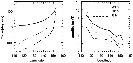
We performed a Fourier analysis on some of the data in Fig. 2, extracting the 24, 12 and 8 hour periods and using the first three days data from 12 to 14 May. Results from the following three days (15–17 May), when available, were similar. The amplitudes and phases are plotted in Fig. 4
as they vary with longitude. The results are similar to
110 120 130 140 150 160
110 120 130 140 150 160
-100 0 100
Longitude
110 120 130 140 150 160
0
110 120 130 140 150 160
-100 0 100
Longitude
110 120 130 140 150 160
0
110 120 130 140 150 160
-100 0 100
Longitude
Fig. 4. Variations with longitude of the phase (left panel) and amplitude (right panel) of three Fourier components derived from Z variation data for 12–14 May 1990 from the stations of Fig. 2.
December 1989 data). Normal expected phase progression would be 1◦of phase for 1◦of longitude for the 24 h period,
2◦ of phase per 1◦ of longitude for the 12 h period and
so on. The outstanding features in Fig. 4 are the fairly abrupt increases in amplitude of all harmonics on the west coast, with some increase also on the east coast, and the rapid phase change on the east coast. If the amplitude and phase are considered as a vector and the “normal” inland station vector is subtracted from the coastal station vector, following the method of Bennett and Lilley (1973), it can be seen that an anomalous Z variation is isolated in both cases, on the west coast on account of the amplitude difference and on the east coast primarily because of the phase difference.
3.
Derivation of “Anomalous” Coastal Z Values
Following Bennett and Lilley (1973) we have calculated
the anomalous vertical component ZA at coastal stations
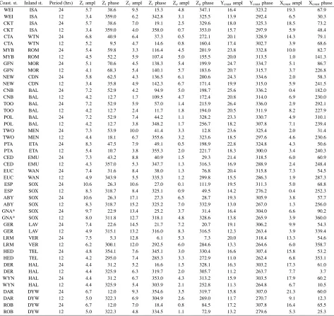
by performing a vector subtraction of Z at a nearby inland station from the Z at the coastal station at a particular fre-quency. Using eight days of hourly data from 6 to 13 De-cember, 1989, we derive the amplitude and phase of the various elements at periods of 24 h and 12 h by perform-ing a least squares fit to the data. Initially we also cal-culated for the 8 h component but found that the error in the fit often exceeded the amplitude. The results are shown in Table 1 where the stations are arranged in order,
travel-ling clockwise around the coast. The time of maximumtm
of each harmonic of periodT is related to the phaseφby
tm =(1/4−φ/360)T. The increased coastal amplitude in
Z, occurring on the west and north coasts, can be seen from ABY up to DAR with the increase in the 12 h harmonic be-ing greater than in the 24 h component. From HED round to DAR the phase of ZAagrees with that of Y at the coastal
stations to within 30◦, except for the 12 h component at
DER where the ZA amplitude is quite small anyway (when
the amplitude of ZA is less than about 2.0 nT its statistical
significance starts to become suspect).
We might try to understand the result at LRM, where the ZA phase is 49◦ahead of Ycoastal, by supposing that it is the
onshore component YO=Ycosθ+Xsinθ which relates to
ZAwhereθis the angle between the coastline and North. In
this case a value ofθ=60◦, for the 24 h component, gives a reasonable value for the phase of ZAto agree with that of the
onshore component YO. This is rather difficult to relate to
the actual coastline, as LRM (Learmonth) is situated within a gulf at a point where the coastline angle changes direction.
Fig. 5. Newcastle plots for 6–13 December 1989 for X, Y, Z and for the onshore component YO.
For the 12 h component there is only a difference of 20◦
between ZAand Y and so the required value ofθwould be
smaller, about 45◦. At GER the angle comes to be about
73◦for the 24 h period and 80◦for 12 h, whereas the actual angle between the coastline and north is more like 30◦.
From ESP round to TOO, that is all along the south coast, the amplitudes of ZA are small and of doubtful statistical
significance, with the exception of TWO.
From CNB up to MYB, on the east coast, the phase
difference between Ycoast and ZA lies between 130◦ and
145◦, except the 12 h harmonic at MYB where it is 158◦. The latter result is an example where it is impossible to find an angleθso that the phase of ZA can be related to an
onshore component, because the amplitude of Xcoastis very small and not significantly different from zero. It follows that any difference between the phases of ZAand Ycoastmust have other physical influences present and the method used above to derive a “theoreticalθ” from the data in Table 1 cannot be considered reliable. The phase relation between Z and the onshore component of Y, YO, can be seen in the
raw data plotted in Fig. 5 where Z at Newcastle is roughly in antiphase to Y at Newcastle and in phase with YO. Here we
estimate the coastline at Newcastle to run at 21.5◦ east of
north so the onshore component will be (Xsin 21.5◦–Ycos
21.5◦).
At ROB, CTA and CKT (12 h harmonic), ZAis
insignifi-cant. WEI is an exception in this region. It might be argued that CTA is quite far from the coast (about 110 km) but a lu-nar ocean effect was detected there (Stening and Hopgood, 1991).
To confirm these results we also calculated the same in-formation for another time period, 12–18 May. As May is more towards the winter season, amplitudes are generally smaller; fewer are large enough to be considered statisti-cally significant. We note here some comparisons. For the GFN/MOR pair, ZAis again significant (6.4 nT for the 12 h
harmonic) and the phase difference between ZAand Ycoastis
128◦, very similar to that in December. For the ABY/SOX
pair and the 12 h harmonic, the ZA and Ycoast phases agree to within 3◦. The CNB/BAL pair also exhibit a similar re-lationship in May as in December.
Finally we performed a few analyses using a larger data
set of 15 days in January 1990, but where Kp reached 3+
Table 1. Amplitudes and phases of 12 and 24 hour components at various stations (6–13 December 1989).
Coast. st. Inland st. Period (hrs) Ziampl Ziphase Zcampl Zcphase Zaampl Zaphase Ycoastampl Ycoastphase Xcoastampl Xcoastphase
WEI ISA 24 5.7 38.6 9.5 15.3 4.8 347.1 16.4 323.2 19.3 67.9
WEI ISA 12 3.4 359.0 6.2 342.8 3.1 325.5 13.9 292.4 6.5 30.3
CKT ISA 24 5.7 38.6 7.0 19.1 2.5 329.6 18.0 325.3 18.5 73.2
CKT ISA 12 3.4 359.0 4.0 358.0 0.7 353.0 15.7 297.9 5.9 48.4
CTA WTN 24 6.8 40.9 6.4 37.3 0.5 272.1 20.1 328.9 14.3 79.1
CTA WTN 12 5.2 9.5 4.7 14.6 0.8 160.4 17.4 302.7 3.9 68.6
MYB ROM 24 5.4 59.8 3.3 116.4 4.5 201.9 23.8 332.8 10.0 82.7
MYB ROM 12 4.5 52.2 5.9 107.4 5.0 155.5 20.0 313.5 1.0 141.3
GFN MOR 24 5.1 70.6 4.5 138.3 5.4 199.9 24.7 334.7 5.1 86.7
GFN MOR 12 4.1 68.3 5.4 140.1 5.7 183.6 20.7 315.7 3.7 226.8
NEW CDN 24 5.8 62.5 4.3 136.5 6.1 200.6 24.3 334.6 2.0 58.3
NEW CDN 12 3.4 35.8 4.9 142.3 6.7 171.4 19.9 315.0 5.9 241.5
CNB BAL 24 7.2 52.9 4.2 94.9 5.0 198.7 25.6 336.2 0.4 182.0
CNB BAL 12 4.2 12.7 1.7 109.5 4.7 172.4 20.8 314.0 6.9 230.0
TOO BAL 24 7.2 52.9 5.9 57.0 1.4 215.9 26.4 336.0 2.9 292.1
TOO BAL 12 4.2 12.7 2.4 11.7 1.8 194.0 20.5 311.9 8.2 227.9
POL BAL 24 7.2 52.9 7.4 44.2 1.1 328.2 23.3 330.7 4.9 310.1
POL BAL 12 4.2 12.7 3.8 348.2 1.7 256.7 18.2 307.8 7.1 239.4
TWO MEN 24 7.3 53.9 10.0 41.4 3.3 12.8 23.6 325.4 2.0 31.4
TWO MEN 12 4.4 18.1 6.7 355.6 3.2 323.6 18.5 297.6 4.6 230.6
PTA ETA 24 8.3 47.5 7.9 49.1 0.5 198.9 22.8 324.8 4.3 50.6
PTA ETA 12 5.4 10.7 3.8 355.3 2.0 221.7 18.3 300.0 3.4 240.3
CED EMU 24 7.3 43.2 8.8 40.9 1.5 29.3 21.4 318.5 6.0 60.9
CED EMU 12 4.3 357.0 5.3 347.7 1.3 316.3 16.9 288.9 2.4 248.4
EUC WAN 24 7.4 31.6 8.4 38.0 1.3 76.8 20.4 315.8 7.3 54.5
EUC WAN 12 4.9 343.9 5.5 335.3 1.2 299.8 15.5 286.3 1.9 287.3
ESP SOX 24 10.6 26.3 10.6 27.0 0.1 111.9 19.5 311.3 5.0 68.8
ESP SOX 12 8.3 318.7 8.4 325.1 0.9 49.5 14.2 276.2 0.4 252.3
ABY SOX 24 10.6 26.3 17.1 27.3 6.5 28.7 19.3 305.9 3.8 57.7
ABY SOX 12 8.3 318.7 15.2 325.2 7.0 332.9 13.0 267.0 1.3 256.0
GNA* SOX 24 9.7 22.9 13.4 25.2 3.7 31.4 16.4 304.0 6.6 90.2
GNA* SOX 12 8.0 311.8 12.7 318.1 4.8 328.6 13.8 265.9 3.9 360.0
GER LAV 24 7.4 22.6 14.5 21.7 7.2 20.7 19.1 306.2 9.9 54.3
GER LAV 12 4.9 315.1 13.2 316.0 8.3 316.5 12.3 263.4 3.9 339.4
LRM VER 24 7.5 5.3 12.8 6.1 5.3 7.3 20.0 318.4 13.3 54.6
LRM VER 12 6.2 300.1 12.0 292.5 6.0 284.6 13.3 264.6 6.0 358.7
HED TEL 24 4.8 354.1 7.6 345.1 3.0 330.4 16.6 307.4 15.8 53.2
HED TEL 12 4.2 295.0 7.4 285.3 3.3 272.9 11.0 262.4 6.8 353.1
DER HAL 24 4.4 31.2 5.2 16.6 1.5 328.1 16.3 303.2 17.3 61.0
DER HAL 12 4.4 325.9 6.3 319.7 2.0 305.7 11.2 263.7 7.7 3.7
WYN HAL 24 4.4 31.2 6.7 353.0 4.3 313.2 15.9 303.5 17.9 60.2
WYN HAL 12 4.4 325.9 5.4 303.9 2.1 252.8 11.3 264.8 6.7 10.5
DAR DYW 24 6.7 12.0 9.3 354.6 3.5 319.7 15.8 307.0 21.3 60.0
DAR DYW 12 5.0 322.3 6.9 304.9 2.6 269.0 11.7 270.7 9.1 12.3
ROB DYW 24 6.7 12.0 7.0 18.4 0.8 84.5 17.2 307.8 16.4 65.5
ROB DYW 12 5.0 322.3 4.8 334.5 1.1 72.9 13.2 279.6 5.3 25.3
*6–9 Dec
Fig. 6. Wyndham X, Y and Z on 6–13 December, 1989 with Wyndham minus Hall’s Creek X to give dX/dφ.
4.
Z Variation where There is Little Coast Effect
At Wyndham (WYN), on the north coast, Z does not clearly correlate well with either of the other components (Fig. 6). Wyndham is actually at the head of Cambridge
Gulf, about 80 km south of the main coastline. However Darwin (DAR) and Wyndham have similar variations in Z, as can also be seen in the phases of their harmonics in Table 1. Figure 6 shows how remarkably the Z variation at WYN changes from day to day. On December 7 and 10 the maxima are larger than the nearby days. These days are different in that the Sq current system focus is at 28–
30◦ latitude while on the other days the focus is around
Fig. 7. X, Y and Z variations at Eucla (EUC) together with an estimate of dX/dφobtained by subtracting X values at Eucla from those at Giles (GIL), 6–13 December 1989.
If the Z variation reflects changes in ionospheric cur-rent strength with latitude, then we might expect a relation between Z and the latitude gradient of the X component dX/dφ. Figure 6 shows that the shape, if not the amplitude, of the Z variation at Wyndham is indeed similar to that of the gradient in X as estimated by differencing the hourly X values at Wyndham (15.5◦S) and Halls Creek (18.2◦S).
We were interested to determine where the changeover
occurred from Z depending on dX/dφto depending on Y.
By visually inspecting variation curves from the December 1989 period for the two pairs DER/TEL and HED/VER we found the change occurred between these two with DER
depending more on dX/dφand HED depending on Y. To
the south the changeover is between Carnarvon (24.9◦S on the west coast) and Geraldton (GER). (The Carnarvon data used were from 12 to 18 May 1990 since that station was not operating in December 1989). Thus visual inspection of the variation curves shows that it is only the small group of stations between Carnarvon and Port Hedland (HED) which exhibit the relation between Z and Y.
We have also examined the records for this December pe-riod from Cooktown (CKT) and Charters Towers (CTA) on the north-east coast. Z at CKT (not shown in a diagram) is remarkably similar to Z at Wyndham, the main difference being a slightly larger post-noon maximum. The morning minimum is clearly visible at CKT. Z at CTA is again sim-ilar but with the morning minimum slightly less prominent. The variations at CTA and MYB are quite different as is evidenced by their phases in Table 1. This change in be-haviour of Z between the north-east and the rest of the east coast shows clearly in the phase lag diagrams of Whellams (1996), both at the 12 and 24 h periods.
On the south coast we would expect Z to be similar to X, if Z reacts to the onshore component, which would be northward. Rarely do we find this to be so.
We will look first at Eucla (EUC) on the south coast. In Fig. 7 we can see no correlation between Z and Y here.
The correlation between Z and dX/dφis better. Here we
estimate dX/dφ by subtracting Eucla X from Giles (GIL)
X. All the deviations are now positive in both Z and dX/dφ. In May X is consistently negative (southward) at Eucla, since the focus is further north during this season, but the Z variation remains positive. The relation of Z to dX/dφin May is also quite good.
At Esperance the agreement between Z and dX/dφis
re-Fig. 8. X and Z variations for 6–13 December 1989 at Esperance (ESP) together with dX/dφfrom subtracting X at ESP from X at Laverton (LAV).
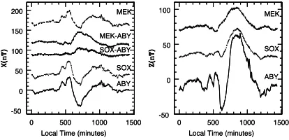
Fig. 9. One minute data for 13 December 1989 of Z (right panel) and X (left panel) for stations in south-west Australia, together with two estimates of dX/dφat Albany (ABY) using X values at MEK and at SOX to subtract from X values at ABY.
markably good (Fig. 8) and, further east at Port Augusta (PTA) Z and dX/dφprovide the best correlation. It there-fore seems that generally, for periods typical of the daily variation, the coast effect is almost absent to the south of the continent. The situation is different at shorter time peri-ods. In Fig. 9 we show an example of this where one minute values are plotted and the higher frequency variations in Z at ABY (periods of about 2 h) relate directly to the X variation
at ABY and not to dX/dφ(as measured by the differences
in X at SOX and ABY or MEK and ABY).
5.
Morning Eastward Current
As mentioned earlier in connection with Fig. 1, an extra eastwards current system often appears in the morning and this has been discussed in detail by Steninget al.(2005a). Evidence of this current system can also be seen in Fig. 6
where, on 8 and 9 December, both Z and dX/dφhave
6.
Discussion
Our concern in this paper is to understand the differ-ent forms of the quiet daily variation Sq(Z) around Aus-tralia. We have found two areas on the east and west coasts where Sq(Z) appears to be somewhat controlled by the
on-shore component of the horizontal variation, YO, though
the phase agreement is not exact. However this effect ap-pears to be restricted in latitude. Other workers have sought to make inferences about the underlying conductivity struc-ture from such information, but this is a complicated mat-ter as the responses are frequency dependent. Here we are mainly interested in periods associated with Sq(Z), that is 24 h and 12 h. In this way we actually came to a different conclusion regarding the variations at Gnangara (GNA) to that of Lilley and Parker (1976). They found the “anoma-lous” component of Z at GNA responded to the onshore
component YO. However the response they found was best
at the shorter 6 h and 8 h periods while at 24 h they obtained a 90◦phase difference which is confirmed by the results in Table 1. This may explain why our results showed Z at Gnangara responding more to dX/dφ.
Around the rest of the coast Sq(Z) seemed to reflect the changes in strength of the overhead ionospheric currents more than induction effects. It is important for researchers to know which stations are significantly affected by induc-tion when they are studying the morphology of ionospheric currents.
The “coastal effect” in Z at periods of 12,24 h is not so simple that it can just be related to the onshore variation YO. Often there is a significant phase difference between
ZA and YOwhich cannot be resolved by adjusting the
an-gle YO makes with the coastline. The region on the east
coast around Newcastle (NEW), where an anomalous Z was identified, coincides with an ocean depth of more than 6 km at less than 100 km from the coast. In comparison ocean depths off the north-east coast and along the south coast are much shallower, often less than 200 m. The situation on the west coast is less clear. For example the 200 m isobath is about 200 km from the coast at HED. We might expect that the coast effect would be more prominent in regions where the ocean is deeper near the coast. However we must recog-nise that the longer period variations are influenced by con-ductivity structures at greater depth. Only sometimes may these deep conductivity structures coincide with coastlines.
7.
Conclusions
1. On parts of the west and east coasts of Australia the daily variation of Z relates mostly to the onshore horizontal component variation, though with some phase difference. On the west coast this effect is restricted to the zone be-tween 20◦S and 30◦S. On the east coast it occurs between 22◦S and about 35◦S.
2. Our results from the north coast show little “coast effect” and the Z variation reflects the change in amplitude with latitude of the overhead east-west ionospheric currents, as measured by the latitudinal gradient in X, dX/dφ. This gradient is likely to be larger at a station between the Sq focus and the equator when the focus is at a lower latitude,
and there is some evidence that this is so.
3. On the south coast Z again mostly follows dX/dφ,
though amplitudes correspond less well than times of max-ima and minmax-ima.
4. Derivation of the anomalous coast effect ZA verified
these findings. However it seemed that ZA was not only
just related to the horizontal onshore component but an additional phase difference was also required at the longer 12, 24 h periods considered here.
5. Different behaviours and relations for shorter period variations were demonstrated.
6. On some days a negative excursion in Z was found in the morning hours, together with a positive X. This indicated an eastward ionospheric current with amplitude increasing towards the pole corresponding to the extra morning current system earlier identified by Steninget al.
(2005a).
Acknowledgments. We thank Drs. Francois Chamalaun and Dr. Charles Barton for making their AWAGS data available. We also thank Dr. Ted Lilley for helpful suggestions and Dr. Jon Turner for programming in connection with Fig. 1. We have appreciated suggestions made by our reviewers.
References
Bennett, D. J. and F. E. M. Lilley, An array study of daily magnetic variations in southeast Australia,J. Geomagn. Geoelectr.,25, 39–62, 1973.
Chamalaun, F. H. and C. E. Barton, The large-scale electrical conductivity structure of Australia,J. Geomag. Geoelectr.,45, 1209–1212, 1993a. Chamalaun, F. H. and C. E. Barton, Electromagnetic Induction in the
Aus-tralian Crust: Results from the AusAus-tralian-Wide Array of Geomagnetic Stations,Exploration Geophysics,24, 179–186, 1993b.
Everett, J. E. and R. D. Hyndman, Geomagnetic variations and electrical conductivity structure in south-western Australia,Phys. Earth Planet. Interiors,1, 24–34, 1967.
Gough, D. I., M. W. McElhinny, and F. E. M. Lilley, A magnetometer array study in Southern Australia,Geophys. J. R Astr. Soc.,36, 345– 362, 1974.
Lilley, F. E. M. and R. L. Parker, Magnetic daily variations compared between the east and west coasts of Australia,Geophys. J. R. Astr. Soc., 44, 719–724, 1976.
Matsushita, S., Solar quiet and lunar daily variation fields, inPhysics of Geomagnetic Phenomena, edited by S. Matsushita and W. H. Campbell, Academic Press, New York, 1967.
Parkinson, W. D. and F. W. Jones, The geomagnetic coast effect,Rev. Geophys. Space. Phys.,17, 1999–2015, 1979.
Srivastava, B. J., H. Abbas, T. RamaGopal, D. R. K. Rao, and B. M. Pathan, Geomagnetic coast and other effects deduced from the new observatory at Visakhapatnam, India,Geophys. J. Int.,146, 827, 832, 2001. Stening, R. J. and P. A. Hopgood, Geomagnetic quiet daily variations in the
Australian region—information from a new station at Charters Towers (20.1◦S),J. Atmos. Terr. Phys.,53, 959–964, 1991.
Stening, R., T. Reztsova, D. Ivers, J. Turner, and D. Winch, Morning quiet-time ionospheric current reversal at mid to high latitudes,Annales Geophysicae,23, 385–391, 2005a.
Stening, R., T. Reztsova, D. Ivers, J. Turner, and D. Winch, A critique of methods of determining the position of the focus of the Sq current system,J. Geophys. Res.,110, A04305, doi: 10.1029/2004JA010784, 2005b.
Whellams, J. M., Spatial inhomogeneity of geomagnetic fluctuation fields and their influence on high resolution aeromagnetic surveys, PhD thesis, Flinders University of South Australia, 1996.