Channel optimized scalar quantizers with erasure correcting codes

R E S E A R C H

Open Access

Channel-optimized scalar quantizers with

erasure correcting codes

Dengyu Qiao

and Ye Li

Abstract

This paper investigates the design of channel-optimized scalar quantizers with erasure correcting codes over binary symmetric channels (BSC). A new scalar quantizer with uniform decoder and channel-optimized encoder aided by erasure correcting code is proposed. The lower bound for performance of the new quantizer with complemented natural code (CNC) index assignment is given. Then, in order to approach it, the single parity check code and corresponding decoding algorithm are added into the new quantizer encoder and decoder, respectively. Analytical results show that the performance of the new quantizers with CNC is better than that of the original quantizers with CNC and natural binary code (NBC) when crossover probability is at a certain range.

1 Introduction

For a uniform scalar source, it is well known from [1] that if over a noiseless channel, in terms of the mean squared distortion (MSD), the uniform scalar quantizer is opti-mal among all quantizers. But if across noisy channels, the uniform quantizer is no longer optimal. Therefore, joint source and channel coding has attracted much atten-tion in [2,3], which has been seen as a promising scheme for effective data transmission over wireless channels due to its ability to cope with varying channel conditions [4-6]. Generally, there are two approaches to improving the performance of a quantizer over a noisy channel.

One is that the encoding cells in quantizer’s encoders are designed to be affected by the transmission channel characteristics, for example [7], or the final positioning of the reconstruction in decoders depends on channel char-acteristics, for example [8], which is called as channel optimized quantizers. In [9-12], some necessary optimal-ity conditions are given. Alternatively, an error detecting code can be cascaded with the quantizer at the expense of added transmission rate in [13].

The other one is index assignment, which is a map-ping of source code symbols to channel code symbols and was studied in [14,15]. The usual goal to design an index

*Correspondence: [email protected]

1Shenzhen Institutes of Advanced Technology, Chinese Academy of Sciences, Shenzhen, China

Full list of author information is available at the end of the article

assignment for noisy channels is to minimize the end-to-end MSD over all possible index assignments. Some famous index assignments, such as natural binary code (NBC), Gray code and randomly chosen index assign-ments, are studied on a binary symmetric channel (BSC) in [16-21]. In [16], it is proved that NBC is optimal for uniform scalar quantizers and uniform source. In [17], McLaughlin et al. extended it to uniform vector quan-tizers. Farber and Zeger [8] also proved the optimality of NBC for uniform source and quantizers with uniform encoders and channel-optimized decoders. In [7], they not only studied on NBC code, but also proposed a new affine index assignment, named as complemented natural code (CNC).

Interestingly, it is known from [7] that for uniform decoder and channel-optimized encoder quantizer with CNC index assignment, as crossover probability increases to a certain value, some of the encoding cells appear to be empty, which is also discovered in [22,23]. These empty cells can be looked upon as redundancy, just like a form of implicit channel coding. Besides, it can be discovered in [7] that there is an implicit assumption is that transmitters should know transition error probabilities. If this assump-tion comes true, then decoders would exactly know the encoding cells in encoders and can judge if the receiving index is one of the indices of empty cells, but [7] does not apply any methods to defeat the receiving index of empty cells.

In this paper, a genie-aided erasure code is applied into the ideal quantizer decoders, which can correct the receiving index of empty cells. The lower bound for per-formance of the uniform decoder and channel-optimized encoder quantizer with CNC index assignment is given. Then, the single parity check (SPC) block code is uti-lized to approach the lower bound. The main scheme is that, in transmitters, several indices are grouped into a block and parity check bits are appended in every block. Afterwards, if a receiving index is detected to be the index of empty cells in receivers, then it will be marked as an erasure. Then, the SPC code is used to correct erasures column by column for every block. In view of the structure, the SPC block code is a little similar to the SPC product code in [24], but their decoders are very different. The decoding scheme of the SPC block code is very simple; thus, only a little complexity will be added.

The rest of this paper is organized as follows. Section 2 gives definitions and notation. In Section 3, the lower bound for distortion of quantizers with uniform decoders and channel-optimized encoders is analyzed. Section 4 introduces the SPC block code and gives the distortion of the quantizer appending it. In Section 5, analytical results are shown. Finally, the conclusion is presented in Section 6.

2 Background

Throughout this paper, a continuous real-valued source random variable X uniformly distributed on [0, 1] is considered. Some of the mathematical notations and definitions follow [7] in this section.Then, a rate n-bit quantizer is a mapping from the source to one of the real-valued codepoints (quantization level) yn(i),

Q:{X|X∈[0, 1]} −→ {yn(i)|i=0, 1,. . ., 2n−1}.

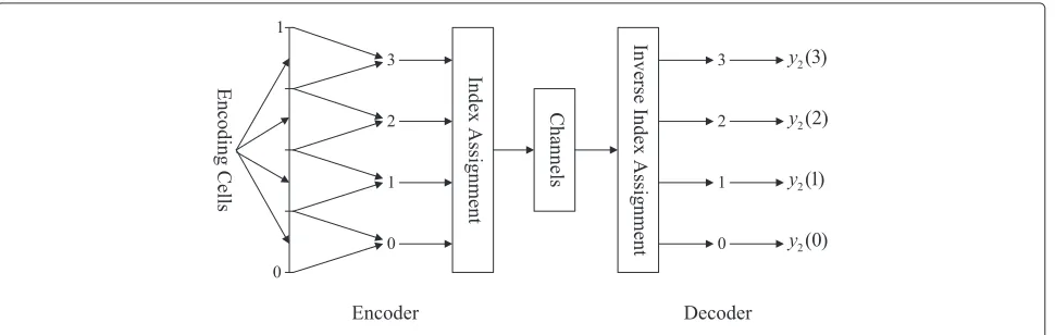
A rate 2 quantizer is plotted in Figure 1 as an example. The quantizer includes a quantizer encoder that is a mapping from sourceXto a certain indexi

Qe:{X|X∈[0, 1]} −→ {i|i=0, 1,. . ., 2n−1},

and a quantizer decoder that is a mapping from the index ito codepointyn(i),

Qd :{i|i=0, 1,. . ., 2n−1} −→ {yn(i)|i=0, 1,. . ., 2n−1}.

In the encoder, theith encoding cell can be denoted by the set

Rn(i)=Q−e1(i).

IfRn(i) = φ, we sayRn(i)is anempty cell. In general,

for most quantizers, there are no empty cells in encoding cells. But a kind of quantizers in [7] is considered, in which the quantizer encoder may contain empty encoding cells. Thecentroidof theith cell of the quantizerQis presented by a conditional expectation

cn(i)=E[X|X∈Rn(i)] .

For a noisy channel, an index assignment π_n is often used to debate noise, which is a permutation of the set {0, 1,. . ., 2n −1}. Then, if indexJis received by a quan-tizer decoder with index assignment, a random variable X∈[0, 1] will be quantized to the quantization level

Qd

π_n−1(J)=yn

π_n−1(J).

Then, the end-to-end mean squared error (MSE) can be written as

D(πn)=E

X−Qd

π_n−1(J)2

. (1)

In this paper, we focus on the quantizers withuniform decodersandchannel-optimized encoders[7]. A quantizer

3

2

1

0 Encoding Cells Index Assignment

Channels

Inverse Index Assignment

3

2

1

0

0 1

2

2

2

2 (3)

(2)

(1)

(0)

y

y

y

y

Encoder Decoder

decoder is said to be uniform if for eachi, theith

code-A quantizer encoder is said to be achannel-optimized encoder if it satisfies the weighted nearest neighbor condition, that is,

Wi⊂Rn(i)⊂Wi, the probability that index j was received, given that indexi was sent. If assuming a binary symmetric chan-nel with crossover probability , pn

tance betweenn-bit binary wordsiandj. Then, according to [7], a quantizer with a uniform decoder and a channel-optimized encoder satisfies, for alli,

Rn(i)= {x∈[0, 1] :αn(i,k)x≥βn(i,k),∀k=i}, (5)

Let an encoder-optimized uniform quantizer (EOUQ) denote a ratenquantizer with a uniform decoder and a channel-optimized encoder, along with a uniform source on [0,1], and a binary symmetric channel with crossover probability. For eachn, the CNC index assignment [7] is defined by

The encoding cells of an EOUQ with the CNC index assignment are given in [7] as follows.

whereδ=1−2.

Ifn≥3 and∈[∗, 1/2), then

Rn(i)=

⎧ ⎪ ⎪ ⎪ ⎪ ⎪ ⎪ ⎪ ⎪ ⎪ ⎪ ⎪ ⎪ ⎪ ⎪ ⎪ ⎪ ⎪ ⎪ ⎨ ⎪ ⎪ ⎪ ⎪ ⎪ ⎪ ⎪ ⎪ ⎪ ⎪ ⎪ ⎪ ⎪ ⎪ ⎪ ⎪ ⎪ ⎪ ⎩

0,δ2−n−_δ2

, fori=0 and <1/2n/2+2

δ2−n−_δ2,4δ+δ22−n−1+

∩[0, 1] , fori=1

2δ(i−1)+δ2

2n+1 +,2δ(i+1)+δ 2 2n+1 +

, for 3≤i≤2n−1−3,iodd

(2n−4) δ+δ2+2n+12−n−1, 1/2, fori=2n−1−1

1/2,(2n+2) δ+1−42+2n+12−n−1, fori=2n−1

2δ(i−1)+1−42

2n+1 +,2δ(i+1)+1−4 2

2n+1 +

, for 2n−1+2≤i≤2n−4,ieven

₍₂n+1_{−6)δ+1−4}2 2n+1 +,

1−2−n_δ+(2−3) δ

∩[0, 1] , fori=2n₋₂

1−2−nδ+ (2−_δ3), 1

∩[0, 1] , fori=2n−1 and <1/2n/2+2

φ, else.

(10)

As above, whenn≥3 and ∈[∗, 1/2), there exists an empty cell set E, which has 2n−1_{−2 elements and consists} of all even numbers from 2 to 2n−1−2 and all odd numbers from 2n−1+1 to 2n−3, given by

E {i:Rn(i)=φ} (11)

= {i: 2≤i≤2n−1−2,ieven} ∪ {i: 2n−1 +1≤i≤2n−3,iodd}.

Let D(πn) denote the end-to-end MSD of EOUQ with

index assignmentπ_n. The MSE of an EOUQ with the CNC index assignment [7] is

D(CNC)=

⎧ ⎪ ⎨ ⎪ ⎩

D1(n,), for 0≤≤∗

D2(n,), for∗≤≤ ₂n/12₊₂

D3(n,), for₂n/12₊₂≤ ≤1/2

, (12)

where

D1(n,)= 2−2n

3(1+2)

₁

4+

22n+5 2

−22n+1−15·2n+42

+622n−2n+2−43+2n−4 2n−24

−122n−45

D2(n,)= 2−3n

3

2n−3+2n−3 22n+10−2n+1+48

−2n−6 2n−5 2n−4−3·22n2

+22n−6 2n−5 2n−43

+122n−5 2n−44+242n−45

D3(n,)= 2−3n

3

2n+3+2n−3 22n+10−2n−1

−2n−6 2n−5 2n−4−3·22n2

+22n−6 2n−5 2n−43

+122n−5 2n−44+242n−45

.

3 Channel-optimized quantizers with erasure correcting codes

As to channel-optimized encoders, the implied key assumption in [7] is that channel state information (CSI) is known to transmitters. In a time division duplexing (TDD) mode system, it is easy to know CSI for transmitters, because uplink and downlink share the same channel. But in a frequency divi-sion duplexing (FDD) mode system, it is much harder to know CSI for transmitters than the TDD mode. Generally, after CSI is estimated in the receivers, it must be fed back to transmitters through an extra reliable channel. Here, in this paper, for a binary symmetric channel, CSI only includes crossover prob-ability . In other words, if the above assumption comes true, for a given channel-optimized encoder in [7], receivers absolutely know temporal and can judge if there exist empty cells in encoding cells and whether the receiving index belongs to empty cells or not. This is because the encoding cells are deter-mined by . Once the empty cell index appears, receivers should recognize that the received index is erroneously detected. However, in [7], the index that is known to be an error is still sent to quantizer decoders.

∀i∈Ec p_nπn

j|πn(i)

=

⎧ ⎪ ⎪ ⎨ ⎪ ⎪ ⎩

pn(πn(i)|πn(i))+k∈Epn(πn(k)|πn(i)) j=i

0 j∈E

pnπnj|πn(i) j∈Ecandj=i

. (13)

Then, similarly, if the proposed quantizer encoder is said to satisfy the weighted nearest neighbor condition, then the encoding cells should satisfy

W_i⊂Rn(i)⊂W_i ∀i∈Ec,

where

W_i= x:_j∈Ec

x−yn

j2pn

πn

j|πn(i)

+_j∈E(x−yn(i))2pn

π_nj|π_n(i)

< _j∈Ecx−y_nj2p_nπ_nj|π_n(k)

+_j∈E(x−yn(k))2pnπnj|πn(k),∀k=i

.

(14)

It is worthwhile to note that the second term in each side of the less-than operator inW_iis different fromWi

in (3). This term means that if receiving an empty cell index, our proposed quantizer decoder is able to correct it. In order to be easier to solve (14), it is rewritten as follows.

Lemma 1. For all i, the encoding cells of our proposed EOUQ satisfy,

R_n(i)=x∈[0, 1] :α_n(i,k)x≥β_n(i,k),∀k=i, (15)

where

α_n(i,k)= j∈Ec

jpn

πn

j|πn(i)

−pn

πn

j|πn(k)

+

j∈E

i·pn

πn

j|πn(i)

−k·pnπnj|πn(k) (16)

β_n(i,k)=2−n−1

⎛

⎝α_n(i,k)+ j∈Ec

j2pn

π_nj|π_n(i)

−pn

πn

j|πn(k)

+

j∈E

i2·pn

πn

j|πn(i)

−k2·pn

π_nj|π_n(k).

⎞ ⎠

(17)

After substituting (8),α_n (i,k)andβ_n(i,k)can be sim-plified as the following two corollaries.

Corollary 1. α_n(i,k)can be simplified as follows. 1. i=0

a.1≤k≤2n−1−1, k odd;2n−1≤k≤2n−2, k even

α_n(0,k)= −k+−2n+2k+2+2n+1−2k−42

+2n−1n−1−2n−1n −2n−k−1pn

2n−2|π_n(k)

+k·pn(0|πn(k))

b. k=2n₋₁

α_n0, 2n−1= −2n+1+2+2n+1−62

+2n+1−2n−1−2n+1−2n

2.1≤i≤2n_{−1, i odd;2}n_−1≤i≤2n_{−2, i even}

a. k=0

α_n(i, 0)=i+2n−2i−2+−2n+1+2i+42

+−2n+1n−1+2n−1n +2n−i−1pn

2n−2|π_n(i)−ipn(0|πn(i))

b.1 ≤ k ≤ 2n−1, k odd;2n−1 ≤ k ≤ 2n−2, k even; k=i

α_n(i,k)=(i−k)−2(i−k) +2(i−k) 2

+2n−i−1pn

2n−2|πn(i)

−i·pn(0|πn(i))−

2n−k−1pn

2n−2|π_n(k)

+k·pn(0|πn(k))

α_n i, 2n−1= −2n−i−1+2n−2i+(2i−2) 2 Appendix (‘The simplification ofβ_n (i,k)’).

It is known from the above two corollaries that for a giveniandk,α_n(i,k)andβ_n(i,k)have only one variable , so the symbolic toolbox inMatlabcan be used to solve

the inequality set. The encoding cellsRn(i)are solved for

Fori∈E, define the quantities

n) denote the end-to-end MSE of modified

EOUQ with index assignmentπnappending a genie-aided

erasure correcting code, which is the lower bound for the MSE of modified EOUQ.

Theorem 3. The lower bound for MSE of a modified EOUQ with the CNC index assignment is

Dlower bound_(CNC) =1

Proof.According to (1) and the assumption we make,

Dlower bound

After re-expressingIl(i)the above formula with respect

toIr(i), and merging like terms according to the

defini-tions ofα_n(i,k)andβ_n(i,k),

After substituting (18) and (19), respectively, Theorem 3 gives the following results.

Theorem 4. The lower bound for MSE of a 3-bit modified EOUQ with the CNC index assignment is

Dlower bound_(CNC) = 5+243+135

2₊₅₇₉3_{−66, 276}6_{+39, 330}5_{−13, 932}4_{+13, 176}9_{−59, 184}8_{+84, 888}7

Theorem 5. The lower bound for MSE of a 4-bit modified EOUQ with the CNC index assignment is

Dlower bound_(CNC) =11, 740+5, 8842−476, 0233 +3, 328, 3444−1, 195, 090, 12212 −5, 134, 292, 76615+4, 009, 702, 08914 −801, 350, 78413+156, 129, 6238 −107, 373, 7497+47, 124, 9396 −14, 855, 9075+1, 183, 613, 61911 −441, 562, 37510−43, 375, 6429 +2, 844, 849, 87016+155, 520, 00019 −518, 967, 00018−143, 067, 60017+52 /12, 2881+304−183−232+11 ×2−304+213−22−3

×1+3+2−2

2+304−433+172−4

(22)

4 EOUQ with CNC aided by single parity check block code

A good erasure code for our proposed quantizers should have excellent ability to correct erasures but no ability to correct errors. This is because the codes that have error correcting ability can improve the performance of not only our proposed quantizers but also the quantizers in [7], and the benefits are equal. Thus, in this section, we focus on SPC code to correct the empty cell index that appears in receivers, in order to approach the lower bound for EOUQ with CNC index assignment.

4.1 SPC Code

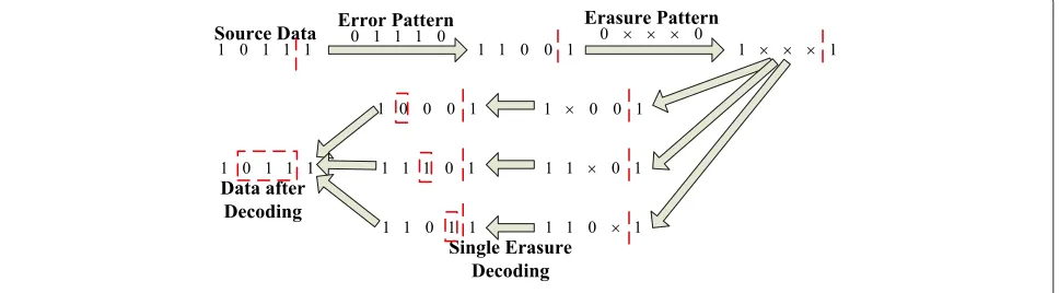
The SPC code is one of the most popular error detection codes for it is easy to be implemented, which is also able to correct a single erasure. But, if there exist multiple era-sures, the typical decoding method for the single-erasure

case will fail to recover them. In this paper, we present a modified decoding method to deal with the multiple-erasure case for the SPC code. The main idea is that when one of the multiple erasures is being recovered, the other erasures are restored to the original value before being marked. Then, the multiple-erasure case can be trans-ferred to several cases for a single erasure. Thus, the typical decoding method for the single-erasure case is still to be effective. Figure 2 gives an illustration of the mod-ified decoding algorithm for the SPC code. According to Figure 2, as multiple erasures are recovered independently if multiple erasures exist, the erasure recovery probabil-ity P˜c with modified decoding method for the

single-or multiple-erasure case is equal to the erasure recovery probabilityPcwith typical decoding method for the

single-erasure case, i.e., ˜

Pc=Pc. (23)

Then, the probabilityPcthat a single erasure can be

recov-ered by the SPC typical decoder is given in the following theorem.

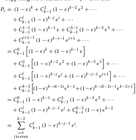
Theorem 6. If a single erasure is detected, the probability that the erasure can be recovered by SPC code is

Pc= ¯ k

j=0

jis even

Cj_k−1(1−)k−j−1j, (24)

where C_nk denotes an n choose k function, k¯ = 2(k−1) /2, and x means to round x to the nearest integers less than or equal to x.

Proof. If a single erasure appears in the receiving SPC code, all error events can be classified into the following several cases.

Case 1. No error: when there exist no errors in the col-umn, the erasure can be definitely recovered. Then, in this case, the recovery probability is(1−)k.

Case 2. One error: when there exists one error in the col-umn, only if the single error happens to be located at the

erasure, the erasure can be recovered. Then, the recovery probability, in this case, is(1−)k−1.

Case 3. Two errors: when there exist two errors in the column, only if the two errors are both not located at the erasure, the erasure can be recovered. Then, the recovery probability, in this case, isC2_k−1(1−)k−22.

Case 4. Odd number of errors: when there existi(odd number) errors in the column, similar to ‘one error case’, only if one of the errors happens to be located at the era-sure, the erasure can be recovered. Then, the recovery probability, in this case, isCi_k−₋1₁(1−)k−ii.

Case 5. Even number of errors: when there existj(even number) errors in the column, similar to ‘two errors case’, only if all errors are all not located at the erasure, the era-sure can be recovered. Then, the recovery probability, in this case, isCj_k−1(1−)k−jj.

In sum, according to all cases, the probability that the single erasure can be recovered by SPC code can be written as

Pc=(1−)k+Ck2−1(1−)k−22+ · · ·

+C_kj₋₁(1−)k−jj+ · · · +C_k1−₋1₁(1−)k−1 +C_k3₋−1₁(1−)k−33+ · · · +C_ki−₋1₁(1−)k−ii+ · · ·,

whereiis an odd number andjis an even number. Assum-ingkis odd, without of generalization, leti=j+1, so that

Pc= (1−)k+Ck2−1(1−)k−22+ · · ·

+C_kj₋₁(1−)k−jj+ · · · +C_k1−₋₁1(1−)k−1 +C_k3−₋₁1(1−)k−33+ · · · +C_kj+₋1₁−1(1−)k−j−1j+1+ · · · =C_k0₋₁

(1−)k+(1−)k−1

+C_k2₋₁(1−)k−22+(1−)k−33

+ · · ·

+C_kj₋₁

(1−)k−jj+(1−)k−j−1j+1

+ · · ·

+C_kk₋−₁1

(1−)k−(k−1)k−1+(1−)k−(k−1)−1k−1+1

=C_k0₋₁(1−)k−1+C_k2₋₁(1−)k−32+ · · · +C_kj₋₁(1−)k−j−1j+C_kk₋−1₁k−1

=

k−1

j=0

jis even

Cj_k−1(1−)k−j−1j.

Supposingkis even, also leti=j+1, so that

Pc= (1−)k+C2_k−1(1−)k−22+ · · ·

+C_kj₋₁(1−)k−jj+ · · ·

+C_k1−₋1₁(1−)k−1+C_k3₋−1₁(1−)k−33+ · · · +C_kj+₋1₁−1(1−)k−j−1j+1+ · · ·

=C_k0₋₁(1−)k+(1−)k−1

+C_k2₋₁

(1−)k−22+(1−)k−33

+ · · ·

+C_kj₋₁

(1−)k−jj+(1−)k−j−1j+1

+ · · ·

+C_kk₋−2₁(1−)k−(k−2)k−2+(1−)k−(k−2)−1k−2+1

=C_k0₋₁(1−)k−1+C_k2₋₁(1−)k−32+ · · · +C_kj₋₁(1−)k−j−1j+C_kk₋−2₁(1−) k−2

=

k−2

j=0

jis even

Cj_k−1(1−)k−j−1j.

Therefore, for anyk≥2, the probability that the single erasure can be recovered by SPC code is

Pc=

2(k−1)/2

j=0

jis even

C_kj₋₁(1−)k−j−1j. (25)

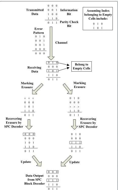
4.2 SPC block code

In this paper,k−1 transmitting indices with parity bits are grouped into a k× nSPC block code, as shown in Figure 3. In a SPC block code, every index is converted to a binary word and then placed row by row, and bits in every column are grouped to a SPC code, respectively. If an index in a row is detected to belong to the empty cell set, all entries in the row are marked as an erasure word. In this paper, erasure word denotes the whole erased bits in one row, and then, a bit in the erasure word is

Information bit

Parity bit

called as erasure bit. Then, the modified SPC decoding method shown in Figure 2 is used to recover every era-sure bit column by column. Figure 4 gives an illustration of the decoding algorithm for a 3-bit quantizer aided by 5×3 SPC block code. As shown in Figure 4, if multiple rows are marked as erasure word, when the erasure words in one row are being recovered, the erasure words in other rows are restored to the original value before being marked.

In order to avoid confusion, we define that I denotes the transmitted index, K denotes the input of the SPC block decoder, and J denotes the output of the SPC block decoder. Then, the SPC block code-aided transition probability p˜nj|i can be defined as

follows.

Theorem 7. If aided by SPC block code, the transition probability p˜n

j|i that index j is output from the SPC

Figure 4An example of decoding algorithm for a 3-bit quantizer aided by 5×3 SPC block code.

block decoder given that index i is transmitted can be written as

˜ pn

j|i=

⎧ ⎪ ⎨ ⎪ ⎩

pn

j|i+_k∈Epn(k|i)

·(1−Pc)Hn(i,j)Pnc−Hn(i,j) j∈E

k∈Epn(k|i)

·(1−Pc)Hn(i,j)Pnc−Hn(i,j) j∈E

.

(26)

Proof.

˜ pn

j|i p˜n

J=j|I=i

= p˜n

J=j,I=i ˜

pn(I=i)

=

kp˜n

J=j,K=k,I=i ˜

pn(I=i)

=

kp˜n

J=j|K =k,I=i· ˜pn(K=k,I=i)

˜ pn(I=i)

=

k

˜

pnJ=j|K=k,I=i· ˜pn(K=k|I=i)

=

k

˜ pn

J=j|K=k,I=i·pn(k|i), (27)

wherepn(k|i)is defined in (4). Obviously,p˜n(K=k|I=i)

=pn(k|i).

Case 1:k∈E (index input into decoders doesnotbelong to empty cells)

˜ pn

J=j|K=k,I=i=

&

1 k=jandj∈E

0 k=j. (28)

This is because if the input index does not belong to the empty cell, it will not be marked as erasure and not be changed by the SPC block decoder.

Case 2: k ∈ E (index input into decoders belongs to empty cells)

In this case,p˜n

to be recovered for an erasure word is equal ton−N. Then,

˜ pn

J=j|K=k,I=i = 1− ˜Pc

N

· ˜Pn_c−N = (1−Pc)N ·Pcn−N (29)

Obviously,N=Hn

i,j, whereHn

i,jis the Hamming distance betweenn-bit binary wordsiandj.

Therefore,

˜ pn

J=j|K=k,I=i=(1−Pc)Hn(i,j)Pcn−Hn(i,j).

(30)

After substituting (28) and (30), (27) can be rewritten as

˜ pn

j|i=

'

pn

j|i+_k∈Epn(k|i)

·(1−Pc)Hn(i,j)Pnc−Hn(i,j) j∈E

k∈Epn(k|i)

·(1−Pc)Hn(i,j)Pcn−Hn(i,j) j∈E

.

(31)

Then, MSD can be written as

DSPC_(CNC) = i

j

˜ pn

π_n(CNC)j|π_n(CNC)(i)

×

(

Rn(i)

x−yn

j2 dx

=

i

j

˜ pn

π_n(CNC)j|π_n(CNC)(i)

×

x3 3 −yn

jx2+y2_njx)))) Rn(i)

.

Now, DSPC_(CNC) is a function of and k. Thus, we can use the Symbolic toolbox in Matlab to obtain the exact expression for every special case as follows.

For 3-bit quantizer,K =3

DK_(CNC=3₎ = 7, 962, 62421−66, 686, 97620 +264, 508, 41619−669, 171, 45618 +1, 226, 192, 25617−1, 745, 986, 75216 +2, 013, 793, 05615−1, 922, 961, 16814 +1, 526, 564, 66413−992, 715, 91212 +509, 652, 36011−192, 400, 66810

+44, 669, 9589−1, 219, 6028−2, 647, 8997 +71, 3076+553, 4495−180, 8464

+4, 0593+2, 7632+501+10 /

768−2+63−32+32 ×1+123−152+32

(32)

For 3-bit quantizer,K=4

DK_(CNC=4₎ = 63, 700, 99224−629, 047, 29623 +2, 944, 180, 22422−8, 785, 760, 25621 +18, 977, 504, 25620−31, 903, 206, 91219 +43, 683, 065, 85618−50, 100, 968, 44817 +48, 911, 316, 48016−40, 974, 579, 64815 +29, 499, 005, 37614−18, 128, 322, 72013 +9, 340, 103, 42412−3, 904, 109, 05211 +1, 250, 869, 33210−273, 128, 5749 +26, 813, 8148+3, 148, 2157+92, 6016 −947, 9255+277, 8304

−7, 5393−3, 7352−501−10 /

−7681+123−152+32 ×−2+63−32+32

(33)

For 3-bit quantizer,K=5

DK_(CNC)=5 = 509, 607, 93627−5, 796, 790, 27226

+31, 484, 215, 29625−109, 374, 603, 26424

+274, 864, 472, 06423−535, 778, 758, 65622

+847, 229, 552, 64021−1, 120, 016, 581, 63220

+1, 262, 654, 369, 28019−1, 229, 166, 254, 59218

+1, 040, 713, 894, 65617−768, 801, 597, 69616

+495, 151, 866, 81615−276, 513, 260, 88014

+132, 315, 403, 41613−53, 156, 640, 28812

+17, 336, 334, 38411−4, 320, 019, 99210

+713, 651, 9709−39, 095, 6348

−11, 051, 1397+193, 3476+1, 467, 8975

−386, 4424+9, 7113

+4, 7072+501+10/768−2+63

−3 2+321+123−152+32

(34)

For 4-bit quantizer,K=3

DK=3 (CNC) =

14, 276, 736, 000, 00039_{107, 794, 022, 400, 000}38

+290, 417, 114, 880, 0003733, 167, 086, 848, 00036 −2, 096, 081, 266, 694, 40035

+7, 146, 138, 215, 312, 6403411, 787, 493, 179, 759, 55233 +4, 294, 650, 642, 726, 52832

+30, 745, 837, 163, 362, 60831_{93, 407, 604, 210, 871, 728}30

+152, 012, 048, 832, 668, 19629160, 041, 493, 676, 832, 38428 +101, 864, 889, 812, 630, 04027

−14, 665, 606, 004, 624, 67026_{45, 599, 458, 954, 787, 901}25

+54, 961, 029, 779, 720, 82924 −31, 880, 510, 555, 625, 80723 +7, 071, 644, 674, 463, 06422

+4, 425, 365, 815, 868, 58321 −5, 028, 119, 456, 259, 99820

+2, 223, 302, 804, 647, 54119_{234, 761, 920, 605, 312}18

−379, 032, 669, 202, 82117

+2, 665, 837, 646, 46012_{154, 116, 255, 422}11

−97, 607, 466, 95610+50, 967, 593, 269916, 469, 653, 1078 +4, 300, 904, 8587−1, 004, 660, 0756

+202, 215, 8445_{22, 094, 182}4_{1, 646, 856}3_{+400, 968}2

+48, 104+208) /

12, 2882+304433+17242

1+304183232+112−2+304213+22+32

1+3₊2₋₂2

(35)

For 4-bit quantizer,K=4

DK=4 (CNC) =

114, 213, 888, 000, 00042_{−1, 033, 673, 011, 200, 000}41 +3, 285, 980, 835, 840, 00040_{−427, 035, 193, 344, 000}39 −29, 615, 491, 894, 579, 20038_{+103, 980, 817, 090, 897, 920}37 −164, 725, 822, 832, 887, 29636_{+34, 515, 810, 866, 297, 088}35 +472, 361, 930, 923, 112, 06434−1, 315, 712, 396, 208, 910, 65633

+2, 125, 947, 487, 263, 270, 81632_{−2, 411, 219, 122, 612, 440, 912}31 +1, 921, 993, 430, 825, 213, 59230_{−851, 450, 424, 470, 925, 900}29 −285, 553, 775, 320, 155, 90028+988, 348, 010, 466, 804, 58827

−1, 071, 182, 372, 882, 329, 48826_{+716, 211, 751, 000, 262, 427}25 −268, 380, 717, 446, 800, 43724_{−24, 693, 601, 109, 397, 063}23 +117, 058, 813, 839, 308, 18422_{−91, 679, 254, 830, 762, 285}21 +40, 953, 822, 541, 585, 40620_{−8, 513, 469, 892, 437, 467}19 −2, 817, 431, 401, 552, 60818_{+3, 612, 067, 778, 674, 335}17 −1, 903, 032, 054, 185, 67216_{+647, 855, 202, 371, 522}15 −132, 028, 998, 320, 98914_{−1, 029, 960, 719, 786}13 +13, 574, 222, 503, 84812_{−6, 451, 548, 073, 534}11 +1, 919, 139, 169, 13010_{−412, 300, 519, 087}9

+64, 933, 542, 8138_{−7, 683, 962, 162}7_{+1, 043, 876, 171}6 −249, 828, 0525_{+40, 140, 886}4_{+201, 576}3

−467, 3042_{−48, 104−208}

/−12, 2881+3₊2₋₂2

−2+304₋₂₁3₊₂2₊₃2

2+304₋₄₃3₊₁₇2₋₄2

1+304₋₁₈3₋₂₃2₊₁₁2

(36)

For 4-bit quantizer,K=5

DK=5

(CNC) =

208+48, 104+533, 6402_{+1, 165, 656}3

−58, 458, 9824_{+281, 191, 396}5

−1, 006, 697, 8676_{+15, 450, 699, 362}7

−19, 1847, 469, 5998_{+1, 488, 428, 462, 173}9

−8, 189, 718, 621, 52410_{+33, 774, 417, 209, 110}11

−103, 453, 615, 005, 20412_{+207, 719, 199, 032, 498}13

−66, 906, 562, 649, 26714_{−1, 513, 988, 103, 500, 822}15

+7, 587, 789, 874, 788, 17016_{−22, 537, 124, 796, 414, 813}17

+44, 795, 080, 053, 420, 03618_{−45, 411, 147, 473, 877, 727}19

−64, 724, 051, 540, 787, 96220_{+441, 781, 898, 032, 166, 091}21

−1, 209, 986, 072, 300, 463, 73222_{+2, 194, 513, 539, 257, 525, 709}23

−2, 581, 081, 879, 055, 831, 87124_{+852, 406, 151, 910, 028, 791}25

+4, 532, 585, 756, 743, 770, 54626_{−13, 587, 290, 869, 775, 967, 948}27

+23, 129, 883, 155, 269, 680, 86428_{−26, 732, 149, 422, 180, 934, 236}29

+17, 882, 765, 153, 323, 206, 43230_{+4, 450, 563, 097, 100, 665, 344}31

−32, 275, 487, 629, 836, 383, 80832_{+51, 938, 010, 511, 486, 921, 344}33

−53, 591, 598, 103, 908, 331, 77634_{+38, 728, 483, 984, 293, 107, 712}35

−18, 259, 673, 092, 737, 874, 94436_{+3, 150, 966, 289, 987, 906, 560}37

+2, 903, 688, 409, 553, 842, 17638_{−2, 899, 835, 033, 082, 052, 608}39

+1, 258, 694, 025, 775, 349, 76040_{−228, 653, 524, 883, 865, 600}41

−47, 498, 124, 460, 032, 00042_{+39, 377, 206, 149, 120, 000}43

−9, 639, 950, 745, 600, 00044_{+913, 711, 104, 000, 000}45

/

12, 288−2+304₋₂₁3₊₂2₊₃2

1+3+2−22

2+304₋₄₃3₊₁₇2₋₄2

1+304₋₁₈3₋₂₃2₊₁₁2

(37)

5 Distortion analysis

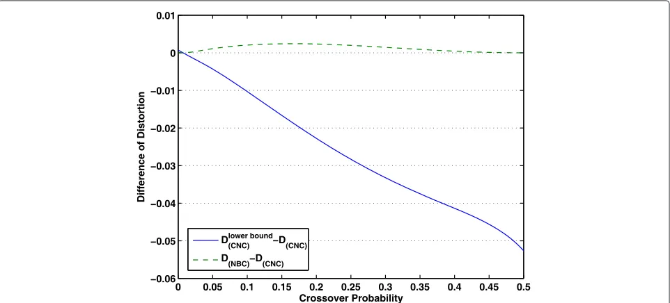
In this section, several figures are plotted to analyze performance of the standard [7] and proposed modi-fied EOUQ. Distortion of the standard EOUQ and the lower bound for distortion of the modified EOUQ with CNC index assignment for 3-bit and 4-bit are shown in Figures 5 and 6, respectively, which are plotted in imi-tation of Figure six in [7] in order to clearly display the difference between those. According to Figures 5 and 6, when the crossover probability is greater than 0.01, the performance of our proposed EOUQ is better than that of the standard EOUQ with CNC index assign-ment, which shows the benefit obtained from a good erasure correcting code. Additionally, when < 0.01, the proposed one is worse than the standard one. This is because the modified EOUQ would increase the quan-tization error due to the fixed empty cells for all in (18) and (19). But this problem can be solved by switch-ing work mode in encoders and decoders. As mentioned before, the difference between the standard and proposed EOUQ is that an erasure correcting code into encoders and the corresponding decode scheme into decoders are appended. So, in a practical system, we can initially give a threshold value ˆ_n for, for example, ˆ_n = 0.01 for 3-bit and 4-bit quantizers. When < ˆ_n, the stan-dard quantizer is adopted. Then, when encoders and decoders realize ≥ ˆn, an erasure correcting code is

appended.

0 0.05 0.1 0.15 0.2 0.25 0.3 0.35 0.4 0.45 0.5 −0.03

−0.025 −0.02 −0.015 −0.01 −0.005 0 0.005

Crossover Probability

Difference of Distortion

Dlower bound_(CNC) −D_(CNC)

D

(NBC)−D(CNC)

Figure 5The difference between EOUQ and proposed modified EOUQ in MSE achieved by CNC index assignment for raten=3.

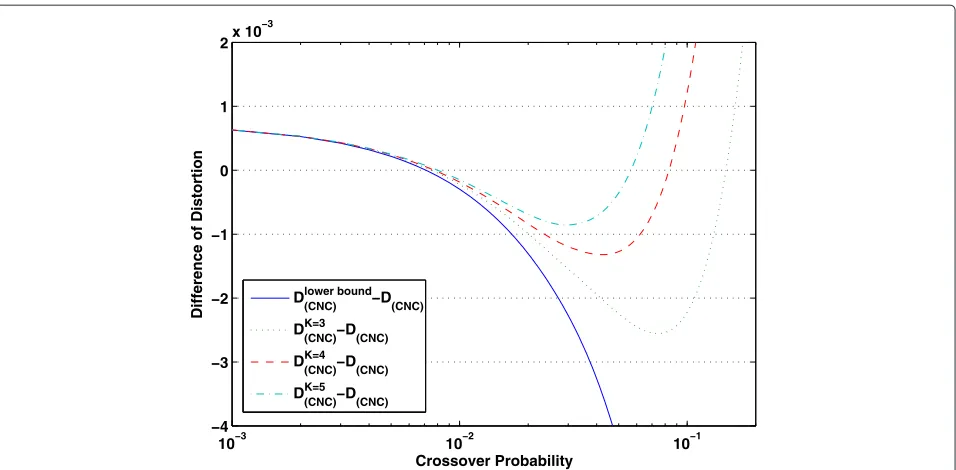
the SPC block decoder does not have enough capabil-ity of correcting all erasures so that a few of empty cell indices cannot be recovered according to Theorem 6. This is a performance penalty incurred by the sub-optimal erasure correcting code used in this paper. If another well-designed SPC code that can increase recovery prob-ability in Theorem 6, for example SPC product code, or better erasure correcting code is adopted, the perfor-mance will approach the lower bound. But it is impor-tant that when crossover probability is numbered from 10−2 to 10−1, the performance of proposed quantizers with CNC index assignment using SPC block code is still

better than that of standard quantizers with CNC index assignment.

6 Conclusion

In this paper, the lower bound for a modified uniform decoder and channel-optimized encoder quantizer with CNC index assignment is proposed. After appending the SPC block code and its decoding algorithm into encoders and decoders, respectively, the performance of this mod-ified quantizer approaches the lower bound and is better than that of the standard quantizer when crossover error probabilityis greater than a thresholdˆ_n.

0 0.05 0.1 0.15 0.2 0.25 0.3 0.35 0.4 0.45 0.5

−0.06 −0.05 −0.04 −0.03 −0.02 −0.01 0 0.01

Crossover Probability

Difference of Distortion

Dlower bound (CNC) −D(CNC) D_(NBC)−D_(CNC)

10−3 10−2 10−1

Difference of Distortion Dlower bound(CNC) −D(CNC)

DK=3

Figure 7The MSE difference between original and modified EOUQ appending a SPC block withK=3, 4, 5 for raten=3.

Appendix

Proof of Lemma 1

Proof. For any integeri,k ∈ [0, 2n−1] buti = k, the inequality in (14) can be rewritten as

Merging like terms gives

x2

After canceling terms and substituting (2), the left side of the inequality gives

10−3 10−2 10−1 −4

−3 −2 −1 0 1 2x 10

−3

Crossover Probability

Difference of Distortion

Dlower bound

(CNC) −D(CNC)

DK=3

(CNC)−D(CNC)

DK=4

(CNC)−D(CNC)

DK=5

(CNC)−D(CNC)

Figure 8The MSE difference between original and modified EOUQ appending a SPC block withK=3, 4, 5 for raten=4.

and similarly, the right side of the inequality gives

2−2nx

j∈Ec

j2+j+1 4 pn

πnj|πn(i)−pnπnj|πn(k)

+2−nx

j∈E

i2+i+1 4

pnπnj|πn(i)

−

k2+k+1 4

pn

πn

j|πn(k)

=2−n+1β_n(i,k)+2−2n−2

j

pn

πn

j|πn(i)

−pn

πn

j|πn(k)

=2−n+1β_n(i,k).

Therefore, the inequality in (14) can be rewritten as

α_n(i,k)x≥β_n (i,k).

The simplification ofβ_n(i,k)

β_n(i,k)=2−n−1 ⎛

⎝α_n(i,k)+ j∈Ec

j2pnπnj|πn(i)

−pn

πn

j|πn(k)

+

j∈E

i2·pn

πn

j|πn(i)

−k2·pnπnj|πn(k).

⎞ ⎠

Case 1.i=0

a. 1≤k≤2n−1,kodd; 2n−1≤k≤2n−2,keven

β_n(0,k)=2−n−1

&

α_n (0,k)+

22n+2 3 −6·2

n₊ 32

3

+4k2−2n+2−4k

3+2n−8

−8k2+3·2n+1−6k2

+

−22n+4

3 +2

n_+4k2

+−2n+1+2k

−k2

+2n−12n−1−2n−12n +k2pn(0|πn(k))−

2n−12−k2

×pn

2n−2|πn(k)

*

b.k=2n−1

β_n0, 2n−1=2−n−1α_n0, 2n−1−22n−12n

+22n−12n−1+2·22n−8·2n+62

+2n+1−2−2n−12

a.k=0

β_n(i, 0)=2−n−1

&

α_n(i, 0)−

22n+2 3 −6·2

n₊ 32

3 +4i 2

−2n+2−4i

3−2n−8−8i2

+ 3·2n+1−6i2−

₋

22n+4

3 +2

n

+4i2+−2n+1+2i

+i2−2n−12

×n−1+2n−12n−i2pn(0|πn(i))

+2n−12−i2pn

2n−2|πn(i)

*

b. 1≤k≤2n−1,kodd; 2n−1≤k≤2n−2,keven;k=i

β_n(i,k)=2−n−1

&

α_n(i,k)+−4i2+4k2+2n+2−4

×(i−k)]3+8i2−8k2 +−3·2n+1+6(i−k)2 +−4i2+4k2+2n+1−2(i−k) ×+i2−k2−i2pn(0|πn(i))

+2n−12−i2

pn

2n−2|π_n(i)

+k2pn(0|πn(k))−

2n−12−k2

×pn

2n−2|π_n(k) *

c.k=2n−1

β_ni, 2n−1=2−n−1 &

α_ni, 2n−1− ₂2n+2

3 −6·2

n

+ 32 3 +4i

2₋₂n+2_−4i

3

+22n+1−9·2n+14+8i2 +−3·2n+1+6i2

+

22n−10

3 +2

n_−4i2₊₂n+1_−2i

×+i2−2n−12 +2n−12n−1−2n−12 ×n−i2pn(0|πn(i))

+2n−12−i2pn

2n−2|πn(i)

*

Case 3.i=2n−1 a.k=0

β_n2n−1, 0=2−n−1α_n2n−1, 0+22n−12n

−22n−12n−1−2·22n−8·2n+62

−2n+1−2+2n−12

b. 1≤k≤2n_{−1,kodd; 2}n_−1≤k≤2n_−2,keven

β_n2n−1,k=2−n−1 &

α_n2n−1,k+ ₂2n+2

3 −6·2

n₊32

3 +4k2−2n+2−4k3

−22n+1−9·2n+14+8k2 +−3·2n+1+6k2

−

22n−10

3 +2

n_−4k2₊₂n+1_−2k

×−k2+2n−12−2n−12n−1

+2n−12n+k2pn(0|πn(k))

−2n−12−k2pn2n−2|πn(k)*

Proof of Corollary 1

In order to prove Corollary 1, the following corollaries will be firstly evidenced.

Corollary 3. If0≤i≤2n_{−1, then}

2n−1

j=0

jpnj|i=2n−1+i(1−2), (38)

and

2n₋₁

j=0

jpn

π_n(CNC)j|π_n(CNC)(i)

=

&

(2n−1) +(1−2) (i+), for i even (2n−1) +(1−2) (i−), for i odd.

(39)

Corollary 3 was proved in [7].

Corollary 4.

2n₋₄

j=2

jeven

jpn

j|i=

⎧ ⎪ ⎪ ⎨ ⎪ ⎪ ⎩

(2n₋₂₎ n₋₍₂n₋₂₎ n−1₋₍₂n₋₂₎ 2₊₍₂n_{−2) i=0}

(2n−2) 2+(i−1) (1−2) −(2n−2)pn(2n−2|i) 1≤i≤2n−1and i is odd

(2n−2) (1−)2−(2n−2) (1−)n i=2n−2

Ifi=0, then is very similar to the above.

Clearly,

α_n(i,k)=an(i)−an(k). (42)

After substituting (41) foran(i)andan(k)in (42) and

merging like terms,α_n(i,k)is simplified.

Proof of Corollary 2

In order to prove Corollary 2, the following corollaries will be firstly evidenced.

Corollary 6 was proved in [7].

Proof.Ifi=0, then

The proof of the other two cases is similar to the above.

If 1≤i≤2n−1−1 andiodd, then

bn(i)=

2n−1

j=0

j2pn

π_n(CNC)j|i −

2n−4

j=2

jeven

j2pnj|i

− 2n₋₄

j=2n−1

jeven

2j+1pn

j|i+i2

2n₋₄

j=2

jeven

pn

j|i

= 2n₋₁

j=0

j2pn

π_n(CNC)j|i −

2n₋₄

j=2

jeven

j2pn

j|i

−2 2n−4

j=2n−1

jeven

jpnj|i−

⎡ ⎣2

2n−2−1

j=0

pn−2

j))i−1 2

−pn

2n−2|i

⎤ ⎦₊i2

2n₋₄

j=2

jeven

pn

j|i.

The proof of the other two cases is similar to the above.

Clearly,

β_n(i,k)=bn(i)−bn(k). (47)

After substituting (46) forbn(i)andbn(k)in (47) and

merging like terms,β_n(i,k)is simplified.

Competing interests

The authors declare that they have no competing interests.

Acknowledgements

This work was supported in part by the National Natural Science Foundation of China under Grant 81101127 and in part by the Shenzhen Basic Research Funds under Grant JCYJ20120615140419045.

Author details

1_{Shenzhen Institutes of Advanced Technology, Chinese Academy of Sciences,}

Shenzhen, China.2_{Huawei Technologies Co., Ltd., Shenzhen, China.}

Received: 20 May 2013 Accepted: 26 May 2014 Published: 18 June 2014

References

1. A Gersho, R Gray,Vector Quantization and Signal Compression(Kluwer, Norwell, MA, 1991)

2. B Hochwald, K Zeger, Tradeoff between source and channel coding. IEEE Trans. Inform. Theory.43(5), 1412–1424 (1997)

3. S Matloub, T Weissman, Universal zero-delay joint source channel coding. IEEE Trans. Inform. Theory.52(12), 5240–5250 (2006)

4. H Wang, S Tsaftaris, A Katsaggelos, Joint source-channel coding for wireless object-based video communications utilizing data hiding. IEEE Trans. Image Process.15(8), 2158–2169 (2006)

5. D Qiao, Y Li, Y Zhang, Energy efficient video transmission over fast fading channels. EURASIP J. Wireless Commun. Netw.2010, 1–12 (2010) 6. Li Ye, M Reisslein, C Chakrabarti, Energy-efficient video transmission over

a wireless link. IEEE Trans. on Vehicular Technol.58(3), 1229–1244 (2009) 7. B Farber, K Zeger, Quantizers with uniform decoders and

channel-optimized encoders. IEEE Trans. Inform. Theory.52(2), 640–661 (2006)

8. B Farber, K Zeger, Quantizers with uniform encoders and channel optimized decoders. IEEE Trans. Inform. Theory.50(1), 62–77 (2004) 9. H Kumazawa, M Kasahara, T Namekawa, A construction of vector

quantizers for noisy channles. Electron. Eng. Jpn.67-B(4), 39–47 (1984) 10. A Kurtenbach, P Wintz, Quantizing for noisy channels. IEEE Trans.

Commun. Technol.COM-17(4), 291–302 (1969)

11. J Zheng, D Rao, Analysis of vector quantizers using transformed codebooks with application to feedback-based multiple antenna systems. EURASIP J. Wireless Commun. Netw.2008, 1–13 (2008) 12. J Dunham, RM Gray, Joint source and noisy channel trellis encoding.

IEEE Trans. Inform. Theory.IT-27(4), 516–519 (1981)

13. J Ho, E-H Yang, Designing optimal multiresolution quantizers with error detecting codes. IEEE Trans. Wireless Com.12(7), 3588–3599 (2013) 14. R Hagen, P Hedelin, Robust vector quantization by a linear mapping of a

block code. IEEE Trans. Inform. Theory.45(1), 200–218 (1999) 15. M Skoglund, On channel-constrained vector quantization and index

assignment for discrete memoryless channels. IEEE Trans. Inform. Theory. 45(6), 2615–2622 (1999)

16. TR Crimmins, HM Horwitz, CJ Palermo, RV Palermo, Minimization of mean-square error for data transmitted via group codes. IEEE Trans. Inform. Theory.IT-15(1), 72–78 (1969)

17. SW McLaughlin, DL Neuhoff, JJ Ashley, Optimal binary index assignments for a class of equiprobable scalar and vector quantizers. IEEE Trans. Inform. Theory.41(6), 2031–2037 (1995)

18. P Knagenhjelm, E Agrell, The Hadamard transform - a tool for index assignment. IEEE Trans. Inform. Theory.42(4), 1139–1151 (1996) 19. A Mehes, K Zeger, Binary lattice vector quantization with linear block

codes and affine index assignments. IEEE Trans. Inform. Theory. 44(1), 79–94 (1998)

20. A Mehes, K Zeger, Randomly chosen index assignments are asymptotically bad for uniform sources. IEEE Trans. Inform. Theory.45(2), 788–794 (1999) 21. X Yu, H Wang, E-H Yang, Design and analysis of optimal noisy channel

quantization with random index assignment. IEEE Trans. Inform. Theory. 56(11), 5796–5804 (2010)

22. N Farvardin, VA Vaishampayan, Optimal quantizer design for noisy channel: an approach to combined source-channel coding. IEEE Trans. Inform. Theory.IT-22(6), 827–838 (1987)

23. N Farvardin, VA Vaishampayan, On the performance and complexity of channel-optimized vector qantizers. IEEE Trans. Inform. Theory. 37(1), 155–160 (1991)

24. DM Rankin, TA Gulliver, Single parity check product codes. IEEE Trans. Commun.49(8), 1354–1362 (2001)

doi:10.1186/1687-1499-2014-99

Cite this article as:Qiao and Li:Channel-optimized scalar quantizers with erasure correcting codes.EURASIP Journal on Wireless Communications and Networking20142014:99.

Submit your manuscript to a

journal and benefi t from:

7Convenient online submission 7Rigorous peer review

7Immediate publication on acceptance 7Open access: articles freely available online 7High visibility within the fi eld

7Retaining the copyright to your article