117
Development of Grey Fuzzy Controller for
Power system Reliability Evaluation Problems
and Preventive Maintenance Suggestions
P
1
P
Ashok kumar Singh, P 2
P
Neelam Sahu
P
1
P
Department of Computer Science, Scholar, Dr. C.V. Raman University, Bilaspur, India
P
2
P
Department of IT, Dr. C.V. Raman University, Bilaspur, India
Abstract
System reliability modeling in terms of fuzzy set theory is basically utilizing the type-2
fuzzy sets, where the fuzzy membership is assumed as point-wise positive function ranging on
[0,1]. Such a practice might not be practical because an interval valued membership may reflect the
vagueness of system better according to human thinking patterns. The Grey fuzzy set is more
capable to handle the uncertainty of system using type-2 fuzzy set.
In this paper, we explore the basics of the GM (1,1) fuzzy sets theory and illustrate its
application in terms of development of reliability models for Power system reliability evaluation
problemsand Preventive Maintenance (PM) suggestions with example.
Keywords
Grey Fuzzy, Reliability Evaluation, Preventive Maintenance (PM)
1. Introduction
System operating and maintenance data are often imprecise and vague. Therefore fuzzy sets
theory (Zadeh 1988) opened the way for facilitating the modeling fuzziness aspect of system
reliability. In this piece of research work, we proposed an effective method to design the power
system stabilizers (PSS). The design of a PSS based on Grey Fuzzy PID Control (PSS+GFPIDC)
can be formulated as an optimal linear regulator control problem however, implementing this
technique requires the design of estimators. This increases the implementation and reduces the
reliability of control system. Therefore, we favor a control scheme that uses only some desired state
variables, such as torque angle and speed. The grey PID type fuzzy controller (GFPIDC) designed
in this paper, can predict the future out put values of the system accurately. However, the
forecasting step-size of the grey controller determines the forecasting value. When the step-size of
the grey controller is large, it will cause overcompensation, resulting in a slow system response.
Conversely, a smaller step-size will make the system respond faster but cause larger overshoots.
The value of the forecasting step-size is optimized according to the values of error and the
derivative of the error. Moreover, the output of the grey controller is updated using the prediction
error for better controller performance. An on-line rule tuning grey prediction fuzzy control system
on-118 line tuning algorithm. The on-line rule tuning grey prediction fuzzy control system structure is
constructed so that the rise time and the overshoot of the controlled system can be maintained
simultaneously.
During the last two decades, grey system theory has developed rapidly and caught the
attention of researchers with successful real-time practical applications. It has been applied to
analysis, modeling, prediction, decision making and control of various systems such as social,
economic, financial, scientific and technological, agricultural, industrial, transportation ,mechanical,
meteorological, ecological, geological, medical ,military, etc., systems. In control theory, a system
can be defined with a color that represents the amount of clear information about that system. For
instance, a system can be called as a black box if its internal characteristics or mathematical
equations that describe its dynamics are completely unknown. On the other hand if the description
of the system is, completely known, it can be named as a white system. Similarly, a system that has
both known and unknown information is defined as a grey system. In real life, every system can be
considered as a grey system because there are always some uncertainties. Due to noise from both
inside and outside of the system of our concern (and the limitations of our cognitive abilities!), the
information we can reach about that system is always uncertain and limited in scope .There are
many situations in industrial control systems that the control engineer faces the difficulty of
incomplete or insufficient information. The reason for this is due to the lack of modeling
information or the fact that the right observation and control variables have not been employed.
A grey predictor with a small fixed forecasting step-size will make the system respond faster
but cause larger overshoots. Conversely, the bigger step-size of the grey predictor will cause over
compensation, resulting in as low system response. In order to obtain a fast system respond with a
little overshoot, the step-size of the grey predictor can be changed adaptively. In the literature of the
grey system theory, there are some methods that tune the step-size of the grey predictor according
to the input state of the system. In order to determine the appropriate forecasting step-size, some
online rule tuning algorithms using a fuzzy inference system have been proposed for the control of
an inverted pendulum ,fuzzy tracking method for a mobile robot and non-minimum phase systems.
In another paper, a Sugeno type fuzzy inference system has been proposed for large time delay
systems.
The power system stabilizers are added to the power system to enhance the damping of the
electric power system.The design of PSSs can be formulated as an optimal line arregulator control
problem whose solution is a complete state control scheme. But, the implementation requires the
design of state estimators. These are the reasons that a control scheme uses only some desired state
variables such torque angle and speed. Upon this, a scheme referred to as optimal reduced order
119 approach retains the modes that mostly affect these variables. In this paper, we adopt a grey model
to predict the output states value. The PID controller is the master controller and the fuzzy control is
the slave control to enhance the master one. Furthermore, we cannot make sure that the forecasting
step size and PID parameters. (Woo.,Chung. and Lin.(2000).)
After the grey system theory was initiated by Deng in1982, Cheng proposed a grey
prediction controller to control an industrial process without knowing the system model in 1986.
From that moment, more and more applications and researches of the grey prediction control were
presented.
The essential concept of this paper is that the fore casting step size in the grey predictor can
be tuned according to the input state of the system during different periods of the system response.
To approach this object, we propose a non-line rule tuning mechanism so that it can quickly
regulate an appropriate negative or positive forecasting step size. A non-line rule tuning algorithm
using the concept of reinforcement learning and supervised learning is proposed to tune the
consequent parameters in the fuzzy inference system such that the controlled system has a desired
out put.
This paper is proposed on-line rule tuning grey prediction fuzzy control system is described
an inverted pendulum control problem is considered to illustrate the effectiveness of the proposed
control scheme.
2. The Structure of Power System Stabilizer
The structure of the grey prediction fuzzy PID control (GFPIDC) power system stabilizer is
composed of five units:
2.1 Grey predictor unit: The grey predictor is used to predict the forecasting values Δ8 and Δ ω,
these values provide the PID and Fuzzy controller.
2.2 Fuzzy controller unit: The fuzzy system is constructed from a set of Fuzzy IF-THEN rules that
describe how to choose the input of PID under certain operation conditions.
2.3 The PID controller unit: The PID controller is using the simple structure in the general
processes. The control signal of power system is generated from this unit.
2.4 The global gain unit: The global gain is obtained from the optimal reduced order model of the
whole system by using only output feedback.
2.5 Online-Tuning unit: An on-line rule tuning algorithm using the concept of reinforcement
learning and supervised learning is proposed to tune the consequent parameters in the fuzzy
120 3. Grey Fuzzy Theory
3.1 Grey System Modeling
Grey numbers, grey algebraic and differential equations, grey matrices and their operations
are used to deal with grey systems. A grey number is such a number whose value is not known
exactly but it takes values in a certain range. Grey numbers might have only upper limits, only
lower limits or both. Grey algebraic and differential equations, grey matrices all have grey
coefficients.
3.2 Generations of Grey Sequences
The main task of grey system theory is to extract realistic governing laws of the system
using available data. This process is known as the generation of the grey sequence. It is argued that
even though the available data of the system, which are generally white numbers, is too complex or
chaotic, they always contain some governing laws. If the randomness of the data obtained from a
grey system is somehow smoothed, it is easier to derive the any special characteristics of that
system. For instance, the following sequence that represents the speed values of a motor might be
given:
X(0) = (200, 300, 400, 500, 600)
It is obvious that the sequence does not have a clear regularity. If accumulating generation is
applied to original sequence, X(1) is obtained which has a clear growing tendency.
X(1) = (200, 500, 900, 1400, 2000)
3.3 GM (n,m) Model
In grey systems theory, GM (n, m) denotes a grey model,where n is the order of the
difference equation and m is the number of variables. Although various types of grey models can be
mentioned, most of the previous researchers have focused their attention on GM (1, 1) model in
their predictions because of its computational efficiency. It should be noted that in real time
applications, the computational burden is the most important parameter after the performance.
3.4 GM (1,1) Model
GM (1,1) type of grey model is most widely used in the literature, pronounced as “Grey
Model First Order One Variable”. This model is a time series forecasting model. The differential
equations of the GM (1,1) model have time-varying coefficients. In other words, the model is
renewed as the new data become available to the prediction model .The GM (1,1) model can only
be used in positive data sequences. In this paper, a non-linear liquid level tank is considered. It is
obvious that the liquid level in a tank is always positive, so that GM(1,1) model can be used to
forecast the liquid level .In order to smooth the randomness, the primitive data obtained from the
system to form the GM(1,1) is subjected to an operator, named Accumulating Generation
121 to obtain the n-step ahead predicted value of the system. Finally, using the predicted value, the
inverse accumulating operation (IAGO) is applied to find the predicted values of original data.
Consider a single input and single output system. Assume that the time sequence 𝑋(0) represents the
outputs of thesystem) x.
𝑋(0) = �𝑥(0)(1), 𝑥(0)(2), … … 𝑥(0)(𝑛)� , 𝑛 ≥ 4 ………..(1)
Where X(0) is a non-negative sequence and n is the sample size of the data. When this
sequence is subjected to the Accumulating Generation Operation (AGO), the following sequence
X(1) is obtained. It is obvious that X(1) is monotoneiP
0)
P
(n) ) , n ≥ 4
𝑋(1) = ��𝑥(1)(1), 𝑥(1)(2), … … 𝑥(1)𝑛�� , 𝑛 ≥ 4… ……… (2)
Where
𝑥(1)(𝑘) = ∑ 𝑥𝑘 (0)(𝑖), 𝑘 = 1,2,3, … . . 𝑛
𝑖=1 …………..(3)
The generated mean sequence Z(1) of X(1) is defined
𝑧(1) = �𝑧(1)(1), 𝑧(1)(2), … … 𝑧(1)(𝑛)� ………(4)
Where z(1)(k) is the mean value of adjacent data, i.e.
𝑧(1)(𝑘) = 0.5𝑥(1)(𝑘) + 0.5𝑥(1)(𝑘 − 1), 𝑘 = 2,3, … . . 𝑛 …………. (5) The least square estimate sequence of the grey difference quation of GM (1,1) is defined as follows:
𝑥(0)(𝑘) + 𝑎𝑧(1)(𝑘) = 𝑏 ……….(6) The whitening equation is therefore as follows:
𝑑𝑥1(𝑡)
𝑑𝑡 + 𝑎𝑥1(𝑡) = 𝑏 ………(7)
In above, [𝑎, 𝑏]𝑇 is a sequence of parameters that can be foundas follows:
[𝑎, 𝑏]𝑇 = (𝐵𝑇𝐵)−1𝐵𝑇𝑌 ………..(8) Where
𝑌 = �𝑥(0)(2), 𝑥(0)(3), ⋯ ⋯ ⋯ , 𝑥(0)(𝑛)�𝑇 …………(9).
𝐵 =
⎣ ⎢ ⎢ ⎢ ⎢
⎡−𝑧(1)(2) 1 −𝑧(1)(2) 1
. . .
−𝑧(1)(𝑛) 1⎦⎥ ⎥ ⎥ ⎥ ⎤
... (10)
According to equation (6.8), the solution of x(1)(t) at time k:
𝑥𝑝(1)(𝑘 + 1) = �𝑥(0)(1) −𝑏𝑎� 𝑒−𝑎𝑘+𝑏𝑎 ……… (11)
To obtain the predicted value of the primitive data at time (k+1), the IAGO is used to
122
𝑥𝑝(0)(𝑘 + 1) = �𝑥(0)(1) −𝑏𝑎� 𝑒−𝑎𝑘(1 − 𝑒𝑎) ………(12)
And the predicted value of the primitive data at time (k+H):
𝑥𝑝(0)(𝑘 + 𝐻) = �𝑥(0)(1) −𝑏𝑎� 𝑒−𝑎(𝑘+𝐻−1)(1 − 𝑒𝑎) ……..(13)
The parameter (a) in the GM (1,1) model is called “development coefficient” which reflects the
development states of X(1)p and X(0)p . The parameter b is called “grey action quantity” which
reflects changes contained in the data because of being derived from the background values.
4. Probability of a Grey Fuzzy System
Grey fuzzy sets are the most widely used type-2 fuzzy sets because they are simple to use
and because, at present, it is very difficult to justify the use of any other kind (e.g., there is no best
choice for a type-1 fuzzy set, so to compound this non-uniqueness by leaving the choice of the
secondary membership functions arbitrary is hardly justifiable). When the Grey fuzzy sets are
interval type-2 fuzzy sets, all secondary grades (flags) equal 1 [e.g.∀𝑓𝑥1�𝑢𝑙𝑖 = 1� and ),∀𝑔𝑥1�𝑤𝑙𝑖 =
1�In this case we can treat embedded type-2 fuzzy sets as embedded type-1 fuzzy sets,so that no new concepts are needed to derive the union, intersection, and complement of such sets. After each
derivation, we merely append interval secondary grades to all the results in order to obtain the final
formulas for the union, intersection, and complement of interval type-2 fuzzy sets. Closed-form
formulas exist for these operations, and their derivations can be found.
The key concept to extend the classical probability calculus toward the fuzzy probability
calculus is the indicator function of a random event A∈ 𝜗, aσ-field of Ω.
𝜗𝐴(𝑤) = � 1 𝑖𝑓 𝜔 ∈ 𝐴0 𝑖𝑓 𝜔 ≠ 𝐴
𝑃𝑟(𝐴) = ∫ 𝜗Ω 𝐴(𝜔)𝑑𝑃 (14)
One fundamental fact is that the right hand is an abstract Lebegue integral. Classical
probability calculus requires random event A is a common subset, i.e., for all ω∈A, such a belonging
relation is definite: it either belongs to A or it does not, there is no middle ground. Therefore
classical probability calculus is short of the capability to describe fuzzy random events. Zedeh
(1965) defined fuzzy set in terms of the extension to indicator function of a normal subset into
membership function of a subset into membership function of a fuzzy set A is mapping from Ω onto
[0,1]
𝜇𝐴: Ω → [0,1].
This mapping is called the membership function of 𝐴̃, whichis a Borel measurable function
representing the degree of element ω belonging to fuzzy set. Thus the probability of fuzzy event is
123
𝑃𝑟�𝐴� = ∫ 𝜇Ω 𝐴(𝜔)𝑑𝑃 (15)
Given a probability space (Ω,𝜗,P), let 𝜑be the collection ofall the fuzzy event on Ω, then (Ω,𝜑,P) is called the induced fuzzy probability space from (Ω,𝜗,P). Therefore, the fuzzyprobability calculus can be established naturally as theextension to the classical probability calculus except
themembership of the interception of two fuzzy events
𝜇𝐴∩𝐵 ≅ 𝜇𝐴, 𝜇𝐵
for maintaining the classical formality of independence, conditional probability, law of total
probability as well as Bayes formula.
5. A Grey Fuzzy Reliability Model of Repairable Systems
A Virtual Allowable Capacity Model for Repairable System
A basic idea of the reliability model proposed here is essentially taking from that of the
traditional power availability-unavailability state modeling of an Electrical power system. If we
treat a repairable system as a virtual electrical power system, then the system parameters, the
maintenance parameters and its operational environment parameters together can form a virtual
allowable capacity, denoted as CRaR, which would restrain or control the system functioning state. The
virtual allowable capacity plays a role similar to the power availability level in the power
availability-unavailability model, which will determine a virtual allowable operating time tRaR,
denoted as PRavR. On the other hand, the system functioning or operating causes system wear-out and
increases its failure hazard. Therefore, the actual system functioning plays a role similar to the
unavailability level, denoted as PRunR.
The limiting state equation of the reliability of functioning power system is:
Z = PRavR− PRunR (16)
Furthermore it is assume that the limiting state Z is normally distributed random variable. It is
intuitive to say that both PRav Rand PRun Rare random and fuzzy in nature. The failure of the system is
assumed to be a Grey fuzzy event with membership function
𝜇RÃR(z)=𝐹𝑂𝑈(Ã) = ∀ 𝑧 ∈ 𝑍 𝜇ÃR(z)=𝐹𝑂𝑈(Ã)= ∀ 𝑧 ∈ 𝑍
6. The Power System Reliability Example
A set of operating data of power system extracted from a Power plant is used. A fuzzy
analysis was performed on the same data in terms of Grey fuzzy set for obtaining the point-wise
124 grades [ 𝜇RĈaR(tRaR), 𝜇RĈaR(tRaR)] by assigning the depth of vagueness π=0.1 atµRÃR(u) =0.5and π=0 at µRÃR(u)
=0 or 1.0. Here Grey membership grades[ 𝜇RĈaR(tRaR), 𝜇RĈaR(tRaR)] are around µRÃR(u) in table 1.
For a recorded failure time or Preventive Maintenance (PM) time, the corresponding the allowable
time satisfies
𝜇𝐶𝑎�(𝑡) = 1 − 𝑡𝑎/𝑡𝑚𝑎𝑥
𝜇𝐶𝑎�(𝑡) = 1 − 𝑡𝑎/𝑡𝑚𝑎𝑥
that is, the allowable time 𝑡𝑎 = 𝑡𝑚𝑎𝑥�1 − 𝜇𝐶𝑎�(𝑡)�
𝑡𝑎 = 𝑡𝑚𝑎𝑥�1 − 𝜇𝐶𝑎�(𝑡)�
Therefore the virtual system state: 𝑧̅ = 𝑡𝑎− 𝑡̅
𝑧 = 𝑡𝑎− 𝑡
For failure times, 𝑡𝑚𝑎𝑥 = 𝑚𝑎𝑥{𝑡1𝑘1, … . , 𝑡31𝑘31} = 147, while for the censoring (PM)
times,𝑡𝑚𝑎𝑥 = 𝑚𝑎𝑥{𝑡1(1 − 𝑘1), … . , 𝑡31(1 − 𝑘31)} = 217,Then�𝜇𝐶𝑎�(𝑡), 𝜇𝐶𝑎�(𝑡)�,�𝑡𝑎, 𝑡𝑎�,and �𝑧, 𝑧̅�,
interval values arecalculated and listed in Table 1.
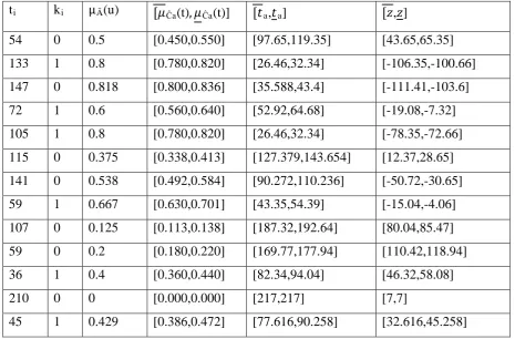
Table 1. "Observed" [𝑡RaR,𝑡RaR]and [𝑧,𝑧]-valued for each PM.
tRi kRi µRÃR(u) [𝜇
RĈaR(t), 𝜇RĈaR(t)] [𝑡RaR,𝑡RaR] [𝑧,𝑧]
54 0 0.5 [0.450,0.550] [97.65,119.35] [43.65,65.35]
133 1 0.8 [0.780,0.820] [26.46,32.34] [-106.35,-100.66]
147 0 0.818 [0.800,0.836] [35.588,43.4] [-111.41,-103.6]
72 1 0.6 [0.560,0.640] [52.92,64.68] [-19.08,-7.32]
105 1 0.8 [0.780,0.820] [26.46,32.34] [-78.35,-72.66]
115 0 0.375 [0.338,0.413] [127.379,143.654] [12.37,28.65]
141 0 0.538 [0.492,0.584] [90.272,110.236] [-50.72,-30.65]
59 1 0.667 [0.630,0.701] [43.35,54.39] [-15.04,-4.06]
107 0 0.125 [0.113,0.138] [187.32,192.64] [80.04,85.47]
59 0 0.2 [0.180,0.220] [169.77,177.94] [110.42,118.94]
36 1 0.4 [0.360,0.440] [82.34,94.04] [46.32,58.08]
210 0 0 [0.000,0.000] [217,217] [7,7]
125
69 0 0.6 [0.560,0.640] [78.12,95.48] [9.12,26.48]
55 0 0.889 [0.877,0.900] [21.7,26.691] [-33.3,-28.309]
74 1 0.875 [0.853,0.888] [16.464,21.609] [-57.536,-52.391]
124 1 0.774 [0.756,0.800] [29.4,35.868] [-94.6,–88.132]
147 1 0.667 [0.630,0.701] [43.953,54.39] [-102.9,-93.345]
171 0 0.375 [0.338,0.413] [127.379,143.65] [-43.621,-27.346]
40 1 0.667 [0.630,0.701] [43.654,54.39] [3.953,14.39]
77 1 0.778 [0.756,0.800] [29.4,35.868] [-47.6,-41.132]
98 1 0.6 [0.560,0.640] [52.92,64.68] [-45.08,-33.32]
108 1 0.6 [0.560,0.640] [52.92,64.68] [-45.08,-33.32]
110 0 0.667 [0.630,0.701] [64.883,80.29] [-45.117,-29.71]
85 1 1 [1.000,1.00] [0,0] [-85,-85]
100 1 0.556 [0.512,0.600] [58.8,71.34] [-41.2,-28.264]
115 1 0.8 [0.780,0.820] [26.46,32.34] [-88.54,-82.66]
217 0 0.2 [0.18,0.220] [169.26,177.94] [-47.74,-39.06]
25 1 0.429 [0.386,0.472] [77.616,90.258] [52.616,65.258]
50 1 0.429 [0.386,0.472] [77.616,90.258] [27.616,40.258]
From the table, it is easy to notice that most of the failure cases (κRiR=1), the �𝑧, 𝑧̅�–valuesobserved
are negative, which indicates the system falls in “failure”and “power unavailable”state,while
quite a few of the censoring cases, the �𝑧, 𝑧̅�-values observed are positive, whichindicates the
system is still in "reliable" and "power available" state. The signs of these "observed"�𝑧, 𝑧̅�
-values confirm that the membership degree of the allowable capacity,�𝜇𝐶𝑎�(𝑡), 𝜇𝐶𝑎�(𝑡)� makesense.
The mean and standard deviation of the interval-valued normal random variable�𝑧, 𝑧̅�can be
accordingly estimated as �𝑚, 𝑚��=[-18.744,-8.853] and �𝜎, 𝜎��=[65.886,66.458] respectively. The
fact that �𝑚, 𝑚�� ≤ 0�clearly indicates the system requires preventive maintenance (PM). Power
System data�𝑡𝑎, 𝑡𝑎�can be used to fit Weibull distributions for further conventional reliability
analysis.
6. Conclusion
The concept of Grey fuzzy system is briefly discussed in this work and argues its necessity
to use Grey fuzzy system idea for the modeling power system reliability. The method of Grey fuzzy
126 the virtual operational state of a power system gives another inside of the power system reliability
status. Using Grey fuzzy system to analyze the power system reliability status and preventive
maintenance suggestions seems more meaningful. As a matter of fact, it is more realistic to
calculate the Grey membership grades and then use the logical function idea to have the Grey
membership grades for the power system reliability status.
References
[1]. Singer, D. (1990). “A fuzzy set approach to fault tree and reliability analysis”. Fuzzy Sets
and Systems, Vol. 34, Issue 2, pp. 145-155.
[2]. Cai, K. Y., Wen, C. Y., and Zhang, M. L. (1991). “Fuzzy variables as a basis for a theory of
fuzzy reliability in the possibility context”. Fuzzy Sets and Systems, Vol. 42, Issue 2, pp.
145-172.
[3]. Cai, K. Y., Wen, C.Y., and Zhang, M. L. (1991). “Posbist reliability behavior of typical
systems with two types of failures”. Fuzzy Sets and Systems , Vol. 43, Issue 1, pp. 17-32.
[4]. Cai, K. Y., Wen, C. Y., and Zhang, M. L. (1991). “Fuzzy reliability modeling of gracefully
degradable computing system”. Reliability Engineering and SystemSafety, Vol. 33, Issue 1,
pp. 141-157.
[5]. Cheng, C. H., and Mon, D. L. (1993). “Fuzzy system reliability analysis by interval of
confidence”. Fuzzy Sets andSystems, Vol. 56, Issue 1, pp. 29-35.
[6]. Chen, S. M. (1994). “Fuzzy system reliability analysis using fuzzy number arithmetic
operations”. Fuzzy Sets and Systems, Vol. 64, Issue 1, pp. 31-38.
[7]. Chen, S. M. (1996). “New method for fuzzy system reliability analysis”. Cybernetics and
Systems: An International Journal, Vol.27, Issue 4, pp. 385-401.
[8]. Chen, S. M. (2003). “Analyzing fuzzy system reliability using interval valued vague set
theory”. International Journal of Applied Science and Engineering, Vol. l, Issue 1, pp.
82-88.
[9]. Mon, D. L., and Cheng, C. H. (1994). “Fuzzy system reliability analysis for components
with different membership functions”. Fuzzy Sets and Systems, Vol. 64, Issue 2, pp.
145-157.
[10]. Pereguda, A.I. (2001). “Calculation of the Reliability Indicators of the System Protected
Object Control and Protection System”. Atomic Energy, Vol. 90, No. 6, pp. 460-468.
[11]. Verma, A.K. et al. (2007). “Fuzzy-Reliability Engineering: Concepts and Applications”.
Narosa Publishing House.
[12]. Ascher, H. E. and Kobbacy, K.A.H.(1995) “Modelling Preventive Maintenance for
Deterirating Repairable System”. IMA Journal of Mathematics Applied in Business &
127 [13]. Baxter, L.A., Kijima, M. and Tortorella M. (1996) “A Point Process Model for the
Reliability of a Maintained System Subject to General Repair”. Communications in
Statistics-Stochatistic Models, Vol.12, Issue 1, 37-65.
[14]. Guo, R. and Love, C.E.(1995) “Bad-As-Old Modelling of Complex Systems with
Imperfectly Repaired Subsystems”. Proceedings of the International Conference on
Statistical Methods and Statistical Computing for Quality and Productivity Improvement,
August 17-19, Seoul, Korea, 131-140.
[15]. Kumar, D. and Westberg, U. (1997) “Maintenance Scheduling under Age Replacement
Policy Using Proportional Hazards Model and TTT-plotting”. European Journal of
Operational Research, Vol. 99, Issue 3, pp.507-515.
[16]. Love, C.E. and Guo, R.(Jan. 1991)“Using Proportional Hazard Modelling in Plant
Maintenance”. Quality and Reliability Engineering International Vol. 7, Issue 1, pp. 7-17.
[17]. Zadeh, A. (June 1965) Fuzzy sets, Information and Control, Vol. 8, Issue 3, 338-353.
[18]. J. M. Mendel and R. I. Bob John (April 2002) “Type-2 fuzzy sets made simple,” IEEE
Trans. on Fuzzy Systems, Vol. 10, No.2, pp. 117-127.
[19]. Q. Liang and J. M. Mendel, (Oct. 2000) “Interval type-2 fuzzy logic systems: theory and
design.” IEEE Trans. on Fuzzy Systems, Vol. 8, No. 5, pp. 535-550.
[20]. N. N. Karnik and J. M. Mendel, (Feb.2001) “Centroid of a type-2 fuzzy set,” Information
Sciences, Vol. 132, Issue 1-4, pp. 195-220.
[21]. J. M. Mendel, (2000) “Uncertainty, fuzzy logic and signal processing,” Signal Proc. J., Vol.