On the Communication Complexity
of Secure Function Evaluation with Long Output
Pavel Hub´aˇcek∗ Daniel Wichs†
Abstract
We study the communication complexity of secure function evaluation (SFE). Consider a setting where Alice has a short inputxA, Bob has an inputxB and we want Bob to learn
some functiony =f(xA, xB) with large output size. For example, Alice has a small secret
decryption key, Bob has a large encrypted database and we want Bob to learn the decrypted data without learning anything else about Alice’s key. In a trivial insecure protocol, Alice can just send her short inputxAto Bob. However, all known SFE protocols have communication
complexity that scales with size of the outputy, which can potentially be much larger. Is such “output-size dependence” inherent in SFE?
Surprisingly, we show that output-size dependence can be avoided in the honest-but-curious setting. In particular, using indistinguishability obfuscation (iO) and fully homo-morphic encryption (FHE), we construct the first honest-but-curious SFE protocol whose communication complexity only scales with that of the best insecure protocol for evaluating the desired function, independent of the output size. Our construction relies on a novel way of using iO via a new tool that we call a “somewhere statistically binding (SSB) hash”, and which may be of independent interest.
On the negative side, we show that output-size dependence is inherent in the fully ma-licious setting, or even already in anhonest-but-deterministic setting, where the corrupted party follows the protocol as specified but fixes its random tape to some deterministic value. Moreover, we show that even in an offline/online protocol, the communication of the online phase must have output-size dependence. This negative result uses an incompress-ibility argument and it generalizes several recent lower bounds for functional encryption and (reusable) garbled circuits, which follow as simple corollaries of our general theorem.
1
Introduction
We study the communication complexity of secure function evaluation (SFE). For simplicity, we focus on the case of a two-party functionality y = f(xA, xB), where Alice and Bob start
with inputsxA, xB respectively and we want Bob to learn the outputy. Alice should not learn
anything about Bob’s input xB or the output y, and Bob should not learn anything about
Alice’s inputxA beyond learning the output y=f(xA, xB).
Traditional approaches to SFE, for example based on Yao garbled circuits [Yao82a], have communication complexity which is proportional to the circuit size of the function f. The breakthrough results on fully-homomorphic encryption (FHE) by Gentry [Gen09] and follow-up works (e.g., [BV11; BGV12; GSW13]) gave the first general SFE solutions whose communication complexity is independent of the circuit size of f, and only scales with the input and output size of f.1
∗
Aarhus University. E-mail: [email protected]. Research supported by ERC Starting Grant 279447 and the CFEM and CTIC research centers. Part of this work was done while visiting the Northeastern University.
†
Communication Complexity of SFE using FHE. Using FHE, we can get SFE solutions whose communication complexity only scales with the input and output size of the functionf
being computed. For example, in the honest-but-curious setting, we get a solution where Bob encrypts his input xB to Alice via a compact and circuit-private FHE for which he knows the
secret key, Alice then runs the computation homomorphically on the received ciphertext and her input xA to get an encryption of y which she sends back to Bob, and Bob decrypts and
learnsy. This achieves communication complexity that scales with |xB|+|y|. Alternatively, we
can get a similar protocol with communication complexity that scales with |xA|+|y|.
More generally, we can take any insecure protocol evaluating a function f with low com-munication complexity and convert it into a secure protocol as follows. Alice and Bob first run a secure distributed key-generation protocol for an FHE scheme, which gives them a common public-key pkand secret-shares skA, skB of the secret keysk=skA⊕skB. They then encrypt
their inputs under pk and execute the insecure protocol for evaluatingf, by running it homo-morphically under the FHE scheme, so that Bob eventually learns an encryption of the output
y. Alice and Bob can then run a secure distributed decryption procedure using their shares
skA, skB and the encryption ofyso that Bob learns the decrypted outputy (but nothing else).
The distributed key-generation and decryption protocols can be implemented generically using an arbitrary SFE scheme.2 IfCC(f) is the best communication complexity for an efficient pro-tocol evaluatingf without any security requirements and λis the security parameter, then the above approach yields an SFE with communication complexitypoly(λ)(CC(f) +|y|) where the
poly(λ) term is some fixed polynomial independent of the functionf. Moreover, using succinct zero-knowledge arguments of Kilian [Kil92], we can even make the above protocols secure in the fully malicious setting without asymptotically increasing the communication complexity.
However, in all known SFE protocols, including the above-described solutions, the commu-nication complexity of the protocol exceeds the output size|y|of the computation. We say that such protocols have “output-size dependence”. As the main question of the paper, we ask if output-size dependence is inherent in SFE.
Is output-size dependence inherent in SFE? If we didn’t require any security, then there is a trivial protocol where Alice just sends her input xA to Bob who computes y =f(xA, xB)
himself, with communication |xA|independent of the output size|y|. Can we achieve this type
of efficiency while maintaining security? For example, imagine that Alice has a short seed x
for a pseudorandom generator (PRG) G, Bob does not have any input, and we want Bob to learn a huge PRG output y = G(x). Can we do this with communication complexity which only depends on |x| but not on|y|? Alternatively, imagine Alice has a small secret decryption key sk, Bob has a large encrypted database c = Encpk(DB) and we want Bob to learn the
plaintext database DB = Decsk(c) without learning anything else about sk. Can we do this
with communication complexity independent of |DB|? In all of these cases, we would like to have an SFE protocol that avoids output-size dependence.
Our Results. On the negative side, we show that output-size dependence is inherent for SFE in the fully malicious setting. In fact, it is already required even in anhonest-but-deterministic
setting, where the corrupted party follows the protocol as specified but fixes its random tape to some deterministic value (say, all 0s). More specifically, we show that in any honest-but-deterministic SFE scheme, the communication from Alice to Bob must exceed the “Yao incom-pressibility entropy” of Bob’s output conditioned on his input, and in general, this can be as large as Bob’s output size. Moreover, we extend this result to protocols in the offline/online setting,
where the parties can run an offline phase before knowing their inputs.3 We show that, no mat-ter how much communication takes place in the offline phase, the communication of the online phase must still satisfy output-size dependence. This negative result uses an “incompressibility argument” which has been used in several recent works giving negative results and/or lower bounds for functional encryption and garbled circuits [AIKW13; AGVW13; DIJ+13; GGJS13; GHRW14]. Our main contribution is to give a (relatively straight-forward) generalization of this technique to proving lower bounds on the communication complexity of general SFE, and then show that all of the prior uses of this technique follow as simple corollaries of our general theorem.
On the positive side, we show that output-size dependence can surprisingly be avoided in the honest-but-curious setting. In particular, using indistinguishability obfuscation (iO) and fully-homomorphic encryption (FHE), we construct the first general honest-but-curious SFE protocols that avoid output-size dependence. We give two such protocols for evaluating an arbitrary function f where Bob learns the output. The first protocol achieves communica-tion poly(λ) +|xA|, where xA is Alice’s input. The second protocol achieves communication
poly(λ)CC(f) which only scales with the communication-complexityCC(f) of the most efficient protocol for evaluating f without any security. In both cases, the poly(λ) term is some fixed polynomial in the security parameterλ, independent of the function f. Since there is always a simple insecure protocol where Alice sends her input to Bob, we haveCC(f)≤ |xA|, and there
are functions for which the gap is large CC(f) |xA|. Therefore the latter protocol may be
better in some instances, although it incurs a multiplicative rather than additive overhead in the security parameter. Using either of these protocols, we get an SFE solution to the problem where Bob has a large encrypted database and wants to securely learn the decryption under a short key held by Alice, using communication complexity which is independent of the database size.
1.1 Our Techniques: Negative Result
Let us begin by describing the technique behind the negative result. For concreteness, consider a two-party computation protocol where Alice has a secret key kfor a pseudorandom function (PRF) fk : N → {0,1}, Bob does not have any input, and we want Bob to learn the PRF
outputs y1 =fk(1), . . . , yL = fk(L) for some large integer L. For contradiction, assume that
we had an SFE protocol for this task where the communication complexity from Alice to Bob is L0 < Lbits. Let’s look at the case where Alice is honest and has a uniformly random key k
as her input, while a corrupted Bob uses an “honest-but-deterministic” strategy, meaning that he follows the specified protocol but fixes his random tape to some deterministic value (say, all 0s). The security of the SFE protocol implies that there is a simulator which gets Bob’s output
y1 =fk(1), . . . , yL=fk(L) and must simulate the view of Bob, denotedviewBob. The simulated
viewBob consists of messages from Alice to Bob (of sizeL0) that cause Bob to outputy1, . . . , yL.
But this means that the simulator canefficiently compress the outputsy1, . . . , yLinto a shorter
string viewBob of size L0 < L bits from which we can efficiently recover the output (by running Bob’s protocol with the fixed randomness). This in turn contradicts the fact that the outputs are pseudorandom and therefore incompressible, showing that such an SFE cannot exist.
As mentioned, our actual result generalize the above example in several ways. Firstly, we show that the communication from Alice to Bob in any SFE for any function f must exceed the “Yao incompressibility entropy” [Yao82b; HLR07] of Bob’s output given Bob’s input. In the above example, the incompressibility entropy of the output is Lbits. Secondly, we extend this result to protocols in the offline/online setting, where we show that the same lower-bound
3
applies to the online phase, no matter how much communication takes place in the offline phase. In this setting, we require that the simulator can simulate the offline phase before the online inputs are chosen, and therefore without knowing the output of the computation.
Lastly, we show that the above negative result implies many prior lower-bounds on func-tional encryption and/or (reusable) garbled circuits. In particular, all of these results follow by showing that the desired primitive would immediately yield an SFE protocol (possibly in the offline/online setting) whose communication complexity would beat our lower bound.
1.2 Our Techniques: Positive Result
Surprisingly, we show that the negative result can be avoided in the honest-but-curious setting.4 Before we describe our solution, it is instructive to see where the negative result fails. In the negative result, we relied on the fact that the simulated view of an “honest-but-deterministic” Bob, denoted viewBob, can be used to reconstruct the output of the function, which consists of pseudorandom valuesy1 =fk(1), . . . , yL=fk(L). Since this view only contained the
communi-cation from Alice to Bob, which we assumed to be shorter than the output sizeL, this served as a compression of the output leading to a contradiction. In the “honest-but-curious” setting, the view of Bob also contains all of his random coins used during the protocol execution, which may be arbitrarily long. Therefore, in this setting, viewBob is no longer compressing even if the communication complexity is small, and the negative result fails.
At first it may appear that the above observation cannot help us. In the real protocol execution, Bob’s coins are truly random and independent of the output; how can we use the random coins to represent/reconstruct the output y1, . . . , yL? We rely on the fact that the
simulator can choose the “simulated random coins” for Bob in a way that is not truly random, and in fact can somehow embed into the random coins information about the outputsy1, . . . , yL,
while still making the coins appear random to a distinguisher.
We now describe our positive result in several steps, focusing on the above example of PRF evaluation for concreteness. This high-level overview doesn’t match the actual constructions in the paper, but it elucidates the main ideas.
First Attempt: Just Obfuscate. As a first attempt, consider a protocol where Alice
con-structs a small circuitCk(i) with a hard-coded keykwhich gets as input an indexi∈ {1, . . . , L}
and outputs fk(i). Alice obfuscates this circuit and sends it to Bob who then evaluates it on
the values 1, . . . , L to get his output. Since the size of the circuit is independent ofL(ignoring logarithmic factors), so is the communication complexity of this protocol. On the positive side, the use of obfuscation might already hide some information about Alice’s input k. On the negative side, there is no hope of simulating this protocol. Indeed, since Bob does not send any communication to Alice, there is no difference between proving the security of this protocol for an honest-but-curious Bob vs. a fully malicious Bob, and our negative result rules this out.
Second Attempt: Hash Randomness then Obfuscate. Our main idea for overcoming
the negative result is to incorporate the random coins of Bob into the protocol. Let’s consider the following modification. Bob first chooses L random bits r1, . . . , rL and hashes them using
a Merkle Tree to derive z = H(r1, . . . , rL). A Merkle Tree has the property that Bob can
efficiently “open” any bit ri of the pre-image by providing a short opening πi. Bob sends the
hashzto Alice. Alice now constructs a small circuit Ck,z(i, ri, πi) that hask, z hard-coded, gets
as input i ∈ {1, . . . , L}, ri ∈ {0,1} and a short opening πi, verifies that πi is a valid opening
of thei’th pre-image bit to ri, and if so outputsfk(i) (if not outputs 0). Alice obfuscates this
circuit Ck,z and sends it to Bob, who then evaluates it on the values i ∈ {1, . . . , L} by also
providing the correct bit ri and the openingπi for each evaluation. The size of the circuit Ck,z
is independent of Land therefore so is the communication complexity of this protocol.
Notice that Bob commits himself ahead of time to providing some random bits ri to the
obfuscated circuit on each evaluation. The circuit checks that it gets the right bit, but then essentially ignores it afterwards. The main idea of the simulation strategy is to choose the random coinsrion behalf of Bob in a way that embeds information about the outputsyiand to
change the circuit being obfuscated so that it uses the inputsri to compute the output without
knowing k. The simulator chooses his own PRF key k0 (unrelated to Alice’s key k which the simulator does not know) and sets the simulated random coins to ri := fk0(i)⊕yi. Then it creates an obfuscation of the circuit Ck00,z(i, ri, πi) which checks the opening πi as before, and
if the opening is valid, it now outputsri⊕fk0(i) instead offk(i). In both cases, if the circuits
Ck,z and Ck00,z get the correct inputs (i, ri, πi) they produce the same outputsyi.
The indistinguishability of simulation boils down to showing that one cannot distinguish an obfuscation of Ck,z and Ck00,z even given r1, . . . , rL, k and k0, where z = H(r1, . . . , rL).
Functionally, these circuits only differ on inputs of the form (i, r0i, π0i) where r0i 6= ri differs
from the bit that was hashed to create z and πi0 is a valid opening. By the security of the Merkle Tree, such inputs are hard to find. Therefore, we could already show the security of the above construction by relying on differing-inputs obfuscation (diO) [BGI+01; ABG+13; BCP14]. However, diO is a strong assumption and there is some evidence that it may not hold in general [GGHW14]. Therefore, we would like a solution based on the weaker and better studied notion of indistinguishability obfuscation (iO) [BGI+01; GGH+13].5
Final Attempt: Hash Carefully and Use iO. It turns out that we can also prove the
security of the above construction using only iO, by being more careful and relying on special type of hash function. We believe that this technique may have broader applicability.
Abstracting out the above construction, we have two circuitsC, C0which have a hard-coded hash-outputz=H(r1, . . . , rL) and they only differ on inputs of the type (i, ri0, πi0) wherer0i6=ri
differs from the hashed bit in position i, and πi0 is a valid opening for ri0. Since the hash is compressing, such inputs necessarily exist. However, we’d like to rely on iO to show that obfuscations ofCandC0 are indistinguishable. We show that we can do this if the hash function satisfies a new notion of security which we call a“somewhere statistically binding” (SSB) hash. An SSB hash Hhk has a short public “hashing key” hk. Just like in a Merkle Tree, we can take z = Hhk(r1, . . . , rL) and, for any position i, produce a short opening πi to certify ri as
the correct bit of the pre-image in that position. Moreover, there is now a method of choosing the hash key hk with a special “binding index” i∗ and we require the following two security properties:
• z = Hhk(r1, . . . , rL) is statistically binding for position i∗, meaning that there does not
exist a valid openingπ0i∗ that would open positioni∗ to the wrong bit r0i∗ 6=ri∗.
• The hash keyhk does not reveal anything about which index i∗ is the binding index.
We show how to construct such SSB hash functions by combining the idea of a Merkle Tree with fully homomorphic encryption. We believe that this primitive may find other applications.
5In both notions of obfuscation, we want to ensure that the obfuscations of two different circuitsC, C0
Using an SSB hash, we show that obfuscations ofCandC0are indistinguishable via a careful hybrid argument. We can define hybrid circuits Ci∗(i, ri, πi) that evaluateC0 when i≤i∗ and
C otherwise, so that C0 = C and CL = C0. For i∗ = 1, . . . , L we define a series of hybrid
distributions where we first change the way we choosehkto be binding on indexi∗and then we change the circuit being obfuscated to Ci∗. Each time we change the circuit being obfuscated from Ci∗−1 to Ci∗, the two circuits being considered are functionally equivalent since the SSB hash is binding on indexi∗. Therefore, we get a proof of security using only iO rather than diO.
General Result. So far, we described a specific example for our positive result where we avoid output-size dependence in the concrete case of PRF evaluation. However, the above ideas generalize to providing a general honest-but-curious two-party SFE protocol for any function
f, so as to achieve the positive results we described previously.
Can Obfuscation be Avoided? We do not know if iO can be avoided in the above positive
result but, in Section 3.4, we present some evidence that at least a weak flavor of obfuscation is inherent. It remains an interesting problem to explore this further and to see what are the minimal assumptions under which we can avoid “output-size dependence” in the honest-but-curious setting.
2
Definitions for SFE
Let f : {0,1}`A(λ) × {0,1}`B(λ) → {0,1}L(λ) be a function family. We consider the secure
function evaluation problem with two parties Alice and Bob, where Alice has a private input
xA∈ {0,1}`A, Bob has a private inputxB ∈ {0,1}`B, and Bob wishes to obtain the evaluation
y=f(xA, xB).
Honest-But-Curious SFE. For our positive result, we will rely on the notion of
honest-but-curious adversaries, where the adversarial party is assumed to follow the protocol specifi-cation completely and hopes to learn some unintended information. For an honest-but-curious
Bob, we define a random variable denoting his view of the protocol by viewΠB(xA, xB, λ) =
(xB, rB, m1, . . . , mt) whererB are the random coins used by Bob, andm1, . . . , mt are the
mes-sages from Alice to Bob. We define the view of an honest-but-curious Alice, viewΠA(xA, xB, λ),
analogously.
Definition 2.1(Honest-But-Curious SFE). We say that two-party protocolΠ securely evaluates
f :{0,1}`A× {0,1}`B → {0,1}Lin the presence of honest-but-curious adversaries, if there exists
a ppt simulator S= (SA, SB) such that for all xA∈ {0,1}`A andxB∈ {0,1}`B it holds that
{simA,λ}λ∈N
c
≈ {viewΠA(xA, xB, λ)}λ∈N , (1)
{simB,λ}λ∈N
c
≈ {viewΠB(xA, xB, λ)}λ∈N , (2)
where simA,λ ←SA(1λ, xA) and simB,λ ←SB(1λ, xB, f(xA, xB)).
We sometimes consider “one-sided” security against honest-but-curious Bob, in which case we only require (2)to hold.
Honest-But-Deterministic SFE. For our negative results, we will rely on a notion of
than the fully malicious one, making our negative results stronger. We will also only consider one-sided security against an honest-but-deterministic Bob, but not require any security against an adversarial Alice. Again, this weakening of the security model makes our results stronger. Lastly, we consider offline/online protocols Π = (Πoff,Πon), comprising of two phases:
• The offline phase protocol Πoff is run independently of the inputs x
A, xB and it allows
the parties to do some pre-processing. Both parties receive their respective inputs only after the end of the offline phase.
• The online phase protocol Πon is run by the parties using their inputs xA, xB and any
state retained from the offline phase. It results in Bob outputting y=f(xA, xB).
We can think of standard SFE protocols as only containing an online phase. We will give a lower-bound on the communication complexity of the online phase in an offline/online protocol, no matter how much communication takes place in the online phase.
The execution of a protocol Π = (Πoff,Πon) between Alice and honest-but-deterministic Bob defines a random variable for Bob’s view of the protocol:
(detviewΠBoff,detviewBΠon)(xA, xB, λ) = ((moff1 , . . . , moffs ),(xB, mon1 , . . . , mont ))
where the offline part consists of the protocol messages from Alice to Bob in the offline phase, and the online part consists of Bob’s input and the protocol messages from Alice to Bob in the online phase. The protocol messages chosen by Alice follow the protocol with true randomness, while those from Bob follow the protocol with the random tape set to the all 0s string.6
Definition 2.2 (Offline/Online SFE Secure against Honest-But-Deterministic Bob). We say that an offline/online two-party protocol Π = (Πoff,Πon) evaluates f : {0,1}`A × {0,1}`B → {0,1}L with security against honest-but-deterministic Bob, if there exists a simulator S = (Soff, Son) such that for all xA∈ {0,1}`A and xB ∈ {0,1}`B it holds that
{simoffB,λ,simonB,λ}λ∈N
c
≈ {(detviewΠBoff,detviewΠBon)(xA, xB, λ)}λ∈N ,
where (simoffB,λ,state)←Soff(1λ) and simB,λon ←Son(xB, f(xA, xB),state).
A crucial but subtle aspect of the above definition for offline/online SFE is that the simulator
Soff must simulate the offline phase without knowing Bob’s input xB or the outputf(xA, xB).
For example, this is required if the inputs can be chosen (e.g., by the adversary/environment) adaptively after the offline phase. In fact, our lower bound in Section 4.2 can be overcome if the simulator is allowed to know the output when simulating the offline part. Indeed Yao garbled circuits (discussed further in Section 4.4) give such an offline/online protocol with low communication complexity in the online part if the offline simulator is given the output.
3
Positive Results in the Honest-But-Curious Setting
We now describe our positive results, giving general SFE protocols in the honest-but-curious setting, whose communication-complexity is independent of the output size of the function being computed. As explained in the introduction, we will rely on a new type of security for hash functions and we begin by describing this new primitive.
6
3.1 Somewhere Statistically Binding Hash Functions
Definition. Asomewhere statistically binding (SSB) hash function allows us to create ashort
hash y =Hhk(x) of some long value x = (x[0], . . . , x[L−1]) and later efficiently “prove” that the i’th block of x takes on some particular value x[i] = u by providing a short opening π. The size of the hashy =Hhk(x), the size of the opening π and the time to verifyπ should be bounded by some fixed polynomials in the security parameter and unrelated to the potentially huge size of x. So far, this problem can be solved using Merkle Trees, where such an opening consists of the hash values of all the sibling nodes along the path from the root of the tree to thei’th leaf. However, the definition of SSB hash has an additional statistical requirement: it allows us to choose the hashing key hk with respect to some special “binding index” i in such a way that the hash y=Hhk(x) is statistically binding on thei’th block of the input, meaning that there only exists a valid opening for a single choice of x[i]. The index ion which the hash is statistically binding should remain hidden by the hashing key hk. The formal definition is below.
Definition 3.1 (SSB Hash). A somewhere statistically binding (SSB) hash consists of ppt
algorithms (Gen, H,Open,Verify) along with a block alphabet Σ = {0,1}`blk, output size `
hash
and opening size `opn, where`blk(λ), `hash(λ), `opn(λ) are some fixed polynomials in the security
parameter. The algorithms have the following syntax:
• hk←Gen(1λ, L, i) takes as input an integer L≤2λ and index i∈ {0, . . . , L−1} (both of these are in binary) and outputs a public hashing key hk.
• Hhk : ΣL → {0,1}`hash is a deterministic polynomial time algorithm that takes as input
x= (x[0], . . . , x[L−1])∈ΣL and outputsH
hk(x)∈ {0,1}`hash.
• π ← Open(hk, x, j): Given the hash key hk, x ∈ ΣL and an index j ∈ {0, . . . , L−1}, creates an opening π∈ {0,1}`opn.
• Verify(hk, y, j, u, π): Given a hash key hk and y ∈ {0,1}`hash, an integer index j ∈ {0, . . . , L − 1}, a value u ∈ Σ and an opening π ∈ {0,1}`opn, outputs a decision ∈ {accept,reject}. This is intended to verify that a pre-image x of y=Hhk(x) has x[j] =u.
We require the following properties:
Correctness: For any integers L ≤ 2λ and i, j ∈ {0, . . . , L−1}, any hk ← Gen(1λ, L, i),
x∈ΣL, π ←Open(hk, x, j): we have Verify(hk, Hhk(x), j, x[j], π) =accept.
Index Hiding: We consider the following game between an attacker Aand a challenger:
• The attackerA(1λ) chooses an integer L and two indices i0, i1∈ {0, . . . , L−1}.
• The challenger chooses a bit b← {0,1} and sets hk←Gen(1λ, L, ib).
• The attackerA gets hk and outputs a bitb0.
We require that for any ppt attacker A we have |Pr[b= b0]− 12| ≤ negl(λ) in the above
game.
Somewhere Statistically Binding: We say that hk is statistically binding for an index i if there do not exist any valuesy, u6=u0, π, π0 s.t. Verify(hk, y, i, u, π) =Verify(hk, y, i, u0, π0) =
accept. We require that for any integers L ≤ 2λ, i ∈ {0, . . . , L −1} the key hk ←
Remarks. Notice that the output size and the opening size of SSB hash are bounded by some fixed polynomials `hash, `opn and independent of the size of the input x. Also, we note
that an SSB hash function is necessarily collision resistant. Intuitively, if an attacker can find
x 6=x0 such that Hhk(x) 6=Hhk(x0)then there must be some index i such that x[i]6=x0[i] and therefore the attacker knows with certainty that the key hk is not binding on index i. This would contradict index hiding. We only make an informal note of this and do not explicitly rely on this property.
Overview of Construction. Our construction combines the ideas behind Merkle Hash Trees
with fully homomorphic encryption (FHE, see Appendix B for a formal definition). Let’s assume we want to hash some data x=x[0], . . . , x[L−1] where L= 2α is a power-of-2. We construct a full binary tree of height α sitting on top of the datax. Each node of the tree is associated with a ciphertext under an FHE scheme. The L leaf nodes are associated with encryptions of x[0], . . . , x[L−1] respectively, where these ciphertexts are computed deterministically using some fixed random coins. The hashing key hk ← Gen(1λ, L, i) consists of an encrypted path in the tree going to a leaf i. Hashing will consist of homomorphically computing a ciphertext for each node of the tree using the ciphertexts associated with its children and the ciphertexts contained in hk. This is done in a way that ensures that all of the ciphertexts on the path from the root to leaf i contain encryptions of x[i]. The output of the hash function is the ciphertext associated with the root of the tree, which is an encryption of x[i] and therefore statistically committing to this value. Analogously to Merkle Trees, opening the hash for some particular block i consist of revealing the ciphertexts associated with all of the siblings along the path from the root to i, which is sufficient to recompute the ciphertext associated with the root. One difficulty is that an adversarial opening may consist of “incorrectly generated ciphertexts” and we cannot guarantee the correctness of homomorphic evaluation over such ciphertexts. Therefore, homomorphic evaluation will only operate on the honestly generated ciphertexts provided as part of the hashing key hk, while the ciphertexts associated with the nodes of the tree will only be used to define the function being evaluated.
Construction. Let E = (KeyGen,Enc,Dec,Eval) be an FHE scheme. For any polynomial
block-size`blk=`blk(λ), we construct an SSB hash function (Gen, H,Open,Verify) with alphabet
Σ ={0,1}`blk as follows.
• hk ←Gen(1λ, L, i): Assume w.l.o.g. that L= 2α is a power-of-2 for some integerα ≤λ. Forj= 0, . . . , α: create (pkj, skj)←KeyGen(1λ). Let (bα, . . . , b1) be the binary represen-tation of the indexi∈ {0, . . . ,2α−1}.7 Forj= 1, . . . , α, computecj ←Encpkj((skj−1, bj)). Lethk= (pk0, . . . , pkα, c1, . . . , cα).
• y = Hhk(x): Let x = (x[0], . . . , x[L−1]). Let T be a binary tree of height α with L leaves. We think of the leaves as being at level 0 and the root of the tree as being at levelα. We inductively and deterministically associate a ciphertext ctv with each vertex
v ∈ T. Intuitively, the encrypted bits bj contained inhk will ensure that the data item
x[i] is propagated up the tree in encrypted form. Formally, we define the ciphertexts ctv
inductively as follows:
– If v is the j’th leaf, we associate to it the ciphertext ctv := Encpk0(x[j]; ¯0) to be a
deterministically computed encryption of x[j] using fixed randomness ¯0.
– Let v ∈ T be a non-leaf vertex at level j ∈ [α] with children v0, v1 having associ-ated ciphertextsct0, ct1, and letcj be the ciphertext contained in hkfor level j. We
7
associate withvthe ciphertextctv =Evalpkj(fct0,ct1, cj) where we define the function:
fct0,ct1(sk, b) : { Compute: x0 =Decsk(ct0), x1=Decsk(ct1).Output xb. }
Note that the functionfct0,ct1 is homomorphically evaluated only over the ciphertext
cj = Encpkj((skj−1, bj)) contained in hk, whereas the ciphertexts ct0, ct1 only serve to define the function being evaluated. The output ciphertext ctv is an encryption
under the keypkj.
The above ensures that for any node v which lies on the path from the root to the leaf at the statistically binding indexi, the associated ciphertext ctv is an encryption ofx[i].
The output of the hash is the ciphertext ctv where v is the root of the treeT.
• Open(hk, x, j): Perform the computation of Hhk(x) as described above and output the ciphertexts ctv for each vertex v that’s a sibling of some vertex along the path from the
root to the leaf at positionj.
• Verify(hk, y, j, u, π): Perform the computation ofHhk(x) as described above using only the provided ciphertexts. In particular, for each vertexv along the path from the root of the tree to leafj, inductively compute a ciphertext ctv. In the base case, when v is thej’th
leaf, setctv =Encpk0(u; ¯0). Otherwise, ifv is not a leaf, than one of its children lies on the
path to leaf j in which case the corresponding ciphertext was computed in the previous step, and the sibling ciphertex is provided in the openingπ. Therefore, we can compute
ctv =Evalpkj(fct0,ct1, cj) wherect0, ct1 are the ciphertexts associated with the children of
v and cj is contained in the hash key hk. Finally, compute the ciphertext ctv associated
with the root of the tree and check thaty =? ctv.
Theorem 3.2. If E = (KeyGen,Enc,Dec,Eval) is an FHE scheme then, for any polynomial block-size `blk(λ), the above construction (Gen, H,Open,Verify) is an SSB hash with
block-alphabet Σ ={0,1}`blk.
Proof. Correctness of SSB hash follows clearly by observation.
For index hiding security, we rely on the semantic security of the FHE scheme. Let i0, i1 ∈ {0, . . . , L1}be the two indices chosen by the adversary Aduring the course of the index hiding game, with binary representationsi0= (bα, . . . , b1) andi1 = (b0α, . . . , b01) respectively. We define a sequence of indistinguishable hybrids that take us from the challenger using the index i0 to
i1. First, we define a sequence of α hybrids where we change the ciphertexts contained in the hashing keyhk= (pk0, . . . , pkα, c1, . . . , cα) fromcj ←Encpkj((skj−1, bj)) toc
∗
j ←Encpkj(¯0) just being an encryption of the all 0 string (starting from j = α and counting down to 1). Then we do another sequence of α hybrids where we change the ciphertexts fromc∗j ←Encpkj(¯0) to
c0j ←Encpkj((skj−1, b
0
j)) (starting fromj= 1 counting up toα). Each pair of successive hybrids
is indistinguishable by the semantic security of the FHE scheme with public key pkj and the
fact that skj is not being encrypted in the two hybrids in question.
Finally, for thesomewhere statistically bindingproperty, we just rely on the correctness of the homomorphic evaluation of the FHE scheme. In particular, assume thathk←Gen(1λ, L, i) con-sists ofhk= (pk0, . . . , pkα, c1, . . . , cα) where (pkj, skj)←KeyGen(1λ) andcj ←Encpkj((skj−1, bj)) where the binary representation ofiisi= (bα, . . . , b1). Assume thatVerify(hk, y, i, u, π) =accept for somey, u, π. During the verification procedure, for each vertexvj at levelj along the path
from the root of the tree to leaf i, we inductively compute a ciphertext ctvj. We claim, by induction, that each such ciphertext satisfies Decskj(ctvj) = u. For j = 0 (base case), the computation sets ctv0 :=Encpk0(u; ¯0), so the claim holds. For each successive j, the
while ct1−bj is provided as part of the opening π and we know nothing about it. By induction
Decskj−1(ctbj) =u. By the correctness of homomorphic evaluation, we therefore have
Decskj(ctvj) =fct0,ct1(skj−1, bj) =Decskj−1(ctbj) =u.
This proves the claim. Therefore, the root ciphertext ctvα = y satisfies Decskα(y) = u. In other word, u is uniquely fixed by y and there cannot exist any u0 6= u and π0 such that
Verify(hk, y, i, u0, π0) =accept. This proves the somewhere statistically binding property.
3.2 One-Sided SFE for Multi-Decryption
In the introduction, we gave an example of a functionality where Alice has a short secret key, Bob has a large encrypted database and we want Bob to learn the decryption without learning anything else about Alice’s secret key. We now show how to do this in the honest-but-curious setting with communication complexity indpendent of the database size. Then, in the next section, we will leverage this protocol to build general SFE schemes.
Multi-Decryption. Let E = (KeyGen,Enc,Dec) be a bit-encryption scheme with ciphertext size`ctx=`ctx(λ). We begin by describing an SFE protocol for the “multi-decryption”
function-ality where Alice has as input a secret keysk ∈ {0,1}`sk and Bob has as input some “database” ofLciphertextsc0, . . . , cL−1 ∈ {0,1}`ctx whereLis some polynomial in the security parameter. The functionality gives Bob the decryptions m0 = Decsk(c0), . . . , mL−1 = Decsk(cL−1) with
mi ∈ {0,1}. In other words, we want an SFE for the function fmulti-decE,L (sk,(c0, . . . , cL−1)) = (m0, . . . , mL−1) where Bob gets the output. We only ask for one-sided security against an
honest-but-curious Bob and do not require any security against a corrupt Alice – she may learn something about Bob’s ciphertexts c0, . . . , cL−1 during the course of the protocol.
Our protocol makes use of an SSB hash function H= (Gen, H,Open,Verify) with alphabet Σ ={0,1}`blk where`
blk :=`ctx+ 1. Assume the SSB hash has some corresponding output size
`hash and opening size `opn (all polynomials in the security parameter λ). The protocol relies
on an indistinguishability obfuscation (iO) scheme O; see Appendix A for a definition of iO. The protocol is given in Figure 1.
Protocol 1. SFE for multi-decryptionfmulti-decE,L (sk,(c0, . . . , cL−1)) = (m0, . . . , mL−1).
• Alice chooses hk←Gen(1λ, L,0) and sendshk to Bob.
• Bob chooses randomness (r0, . . . , rL−1) ← {0,1}L. Let x[i] = (ci, ri) ∈ Σ and x =
(x[0], . . . , x[L−1])∈ΣL. Bob computesy←Hhk(x) and sends y to Alice.
• Alice creates a circuit C =C[hk, y, sk] as described below and obfuscates it by com-puting Ce← O(1λ, C). She sends Ce to Bob.
• Fori= 0, . . . , L−1, Bob computes πi =Open(hk, x, i) and mi :=Ce(i, ci, ri, π).
Figure 1: Protocol for multi-decryption.
Given values hk (hash key), y (hash output) and sk (decryption key) define the circuit
C[hk, y, sk](i, c, r, π): // Hard-coded: hash key hk, hash value y, decryption keysk. // Input: i∈ {0, . . . , L−1},c∈ {0,1}`ctx,r∈ {0,1},π ∈ {0,1}`opn. 1. Check that Verify(hk, y, i,(c, r), π) =accept. If not, output 0.
2. OutputDecsk(c).
In addition, we assume that the circuit C includes some polynomial-size padding to make it sufficiently large. In particular, we also define an augmented circuitCaug =Caug[hk, y, sk, k, i∗] below, which is not used in the protocol, but is used in the proof of security. We will need to pad C so that its size matches that of Caug. For the definition of Caug, we assume thatfk(x)
is a PRF with keyk∈ {0,1}λ, input x∈ {0, . . . , L−1} and output fk(x)∈ {0,1}.
Caug[hk, y, sk, k, i∗](i, c, r, π): //New values: PRF keyk, indexi∗∈ {0, . . . , L−1}. 1. Check that Verify(hk, y, i,(c, r), π) =accept. If not, output 0.
2. If i≥i∗ output Decsk(c), else outputfk(i)⊕r.
Theorem 3.3. If H is an SSB hash and O is an iO scheme then Protocol 1 is a secure
SFE for the functionality fmultiE,L -dec with one-sided security against an honest-but-curious Bob. Furthermore, for any choice of encryption scheme E, there is some polynomial p(λ) such that for every polynomial L(λ) the communication complexity of the above protocol for fmultiE,L -dec is bounded by p(λ) and is independent of L(λ).
Proof. Firstly, we describe the simulator S which gets Bob’s inputs/outputs {ci, mi}Li=0−1 and creates a simulated view simB = ({ri}iL=0−1,hk,Ce) consisting of Bob’s simulated random coins
{ri}and the simulated protocol messages hk,Ce from Alice. The simulatorS chooses a random PRF keyk← {0,1}λ and sets the random coins tori :=fk(i)⊕mifori= 0, . . . , L−1. It chooses
the hashing key hk ← Gen(1λ, L, L−1), sets x := (x[0], . . . , x[L−1]) with x[i] = (ci, ri) and
computes y :=Hhk(x). Finally, it creates a circuit C0 =Caug[hk, y,⊥, k, i∗ =L] (containing⊥ in place of Alice’s secret keysk) and setsCe← O(1λ, C0). Note that, as a quick “sanity check”, when πi =Open(hk, x, i) thenCe(i, ci, ri, πi) =fk(i)⊕ri =mi.
Let’s fix some choice of Alice/Bob inputs: skandc0, . . . , cL−1, which also fixes Bob’s outputs: mi =Decsk(ci).8 LetviewB be the real-world view of an honest-but-curious Bob in the protocol
when interacting with an honest Alice using the above inputs. Let simB ← S({ci, mi}Li=0−1) be the simulated view as described above. We need to show that the real and simulated views are indistinguishable: viewB
c
≈simB. We do so via a sequence of hybrid arguments.
Let Hybrid 0 be the distribution of the real-world view viewB. We define a sequence of
hybrids where we make small modifications and eventually arrive at the distribution of the simulated view simB.
Let Hybrid1 be the same as Hybrid 0, but instead of choosing Bob’s coins ri uniformly
at random, we choose a random PRF key k ← {0,1}λ and we set ri =fk(i)⊕mi. It’s clear
thatHybrid0 and Hybrid1 are indistinguishable by the security of the PRF.
Let Hybrid 2 be the same as Hybrid 1, but instead of obfuscating the circuit C =
C[hk, y, sk] on behalf of Alice, we obfuscate the augmented circuitC0aug=Caug[hk, y, sk, k, i∗ := 0] (containing Alice’s keysk), by settingCe ← O(1λ, C0aug). Note thatC andC0aug compute the same function, and also C was padded to be of the same size as C0aug. Therefore, these two hybrids are indistinguishable by the iO security of the obfuscatorO.
Let Hybrid2.(i, j) for i, j∈ {0, . . . , L} be the same as Hybrid2 except that: (I) instead of obfuscating C0aug, we obfuscate Ciaug =Caug[hk, y, sk, k, i∗ :=i] by setting Ce ← O(1λ, C
aug i )
(II) instead of choosing hk ← Gen(1λ, L,0) we choose hk ← Gen(1λ, L, j) to be statistically
binding at indexj. It’s easy to see thatHybrid2 and 2.(0,0) are identical.
8
We claim that:
Hybrid 2.(i, i) ≈c Hybrid 2.(i+ 1, i) i∈ {0, . . . , L−1} (3)
Hybrid 2.(i+ 1, i) ≈c Hybrid 2.(i+ 1, i+ 1) i∈ {0, . . . , L−2} (4)
To see (3), notice that Ciaug and Ciaug+1 only differ in how they evaluate inputs of the form (i, c, r, π) for which Verify(hk, y, i,(c, r), π) =accept. By the “somewhere statistically binding” property of the SSB hash which is selected to be binding at index i, such inputs must satisfy (c, r) = (ci, ri) where ci is Bob’s i’th input and ri = fk(i)⊕mi. In this case Ciaug outputs
Decsk(c) = mi and Ciaug+1 outputs fk(i)⊕ri = mi, meaning that the circuits behave the same
way on all inputs. Therefore, (3) follows by the iO security of the obfuscation scheme. On the other hand, (4) follows immediately from the index hiding property of the SSB hash function. Together, this shows that Hybrid2 is indistinguishable fromHybrid2.(L, L−1).
Let Hybrid 3 be the same as Hybrid 2.(L, L−1) but instead of obfuscating the circuit
CLaug =Caug[hk, y, sk, k, i∗ =L] we obfuscate the circuitC0 =Caug[hk, y,⊥, k, i∗ =L] (replacing
sk with ⊥). Since sk is never used in either circuit, their behavior is identical, and therefore the indistinguishability of these hybrids follows from the iO security of the obfuscation scheme.
Hybrid 3 is the same as the simulate view simB. Therefore, putting everything together,
we showed that the real/simulated views are indistinguishable viewB c
≈simB, which proves the
theorem.
3.3 General SFE Constructions
We now leverage the protocol for multi-decryption from the previous section to get generic SFE protocols in the honest-but-curious setting. Let
f ={fλ :{0,1}`A(λ)× {0,1}`B(λ)→ {0,1}L(λ)}λ∈N
be any efficiently computable function with `A, `B, L being some polynomials in the security
parameterλ. We focus on SFE schemes where Alice has inputxA, Bob has inputxB and Bob
learns the outputy=f(xA, xB).
We give two constructions. The first one achieves communication complexitypoly(λ)+`A(λ),
where poly(λ) is some fixed polynomial independent of the choice of f or its parameters. In particular, the communication complexity only depends on Alice’s input size`Abut is
indepen-dent of Bob’s input-size`B or output-sizeL. The second construction achieves communication
complexity poly(λ)CC(f, λ) where CC(f, λ) is the communication complexity of an arbitrary insecure protocol for evaluating the functionf andpoly(λ) is some fixed polynomial independent of the choice off or its parameters. Since there is always a simple insecure protocol where Alice sends her input to Bob, we haveCC(f, λ)≤`A(λ) and in general, it may be much smaller than
Alice’s input size. Unfortunately, in this construction we pay with a multiplicative polynomial overhead rather than an additive one as before.
First Construction. LetE= (KeyGen,Enc,Dec,Eval,Rerand) be an FHE scheme with reran-domization (see Appendix B). As discussed in Appendix B, by relying on hybrid encryption we can assume without loss of generality that a ciphertext produced by c ← Encpk(x) is of size
|x|+poly(λ), meaning that there is only an additive polynomial overhead. Our protocol is given in Figure 2.
Theorem 3.4. Assuming that E = (KeyGen,Enc,Dec,Eval,Rerand) is an FHE scheme with
Protocol 2. General SFE Protocol for f ={fλ :{0,1}`A(λ)× {0,1}`B(λ) → {0,1}L(λ)}.
Alice has inputxA, Bob has inputxB and Bob learnsy=f(xA, xB).
• Alice computes (pk, sk)←KeyGen(1λ),cA←Encpk(xA) and sendspk, cA to Bob.
• Bob computescout =Evalpk(f(·, xB), cA). Bob chooses a “one-time-pad”k← {0,1}L
and sets cpad = Evalpk(OTPk, cout) where OTPk(y) := y⊕k. Finally, Bob computes
cf rsh←Rerandpk(cpad). Let cf rsh= (c0, . . . , cL−1) whereci are bit-encryptions.
• Alice and Bob execute Protocol 1 for the functionalityfmulti-decE,L where Alice has input
sk and Bob has inputcf rsh= (c0, . . . , cL−1). Bob receives the outputz∈ {0,1}L and setsy:=k⊕z as the output of the protocol.
Figure 2: First Construction – general protocol fory=f(xA, xB).
secure SFE scheme for any polynomial-time computable functionality f. Furthermore, there is some fixed polynomial p(λ) such that for every such functionalityf where Alice’s input size is
`A(λ), the communication complexity of the protocol is given by p(λ) +`A(λ).
Proof. The communication complexity of the protocol follows by observation and relying on the fact that we can take any FHE scheme and ensure that the ciphertext-size only incurs an additive overhead, meaning that |cA|= `A(λ) +p(λ) for some fixed polynomial p(λ). See
Appendix B for details.
To simulate an honest-but-curious Bob, the simulator chooses (pk, sk) ← KeyGen(1λ) and setscA←Encpk(0`A) to be an encryption of the all 0 string on behalf of Alice. It then runs Bob’s
honest protocol with fresh randomness to compute cout, cpad, cf rsh as Bob would do. Finally it
simulates the execution of Protocol 1 using the one-sided simulator for that protocol, where Bob has input cf rsh = (c0, . . . , cL−1) and output y = (y0, . . . , yL−1) ∈ {0,1}L. It is clear that this is indistinguishable by the semantic security of the FHE scheme and the simulation-security of Protocol 1.
To simulate an honest-but-curious Alice, the simulator runs Alice’s protocol to produce the first round messages pk, cA. It then chooses randomness z ← {0,1}L and computes cpad ←
Encpk(z) and cf rsh ← Rerandpk(cpad). Finally, it runs a real execution of Protocol 1 between
Alice and Bob where it uses the inputcf rshon behalf of Bob. Notice that in the real protocolz=
y⊕khas the same distribution asz← {0,1}L in the simulation. Furthermore, in both the real protocol and the simulation, cf rshis derived by runningRerandpk(cpad) on some ciphertextcpad
such that Decsk(cpad) =z. The only difference between the real execution and the simulation
is that cpad is computed completely differently. By the security of rerandomization, this is
indistinguishable.
Second Construction. Let πinsecf = (πA, πB) be any (insecure) protocol between Alice and Bob that evaluates the functiony=f(xA, xB) so that Bob learnsy at the end of the protocol.
We assume that it has some fixed round complexity q =q(λ) and fixed communication-length in each round, independent of the particular inputs. Without loss of generality, the protocol π
works as follows: Alice and Bob start out with a state that just consists of their inputsstateA0 =
xA,stateB0 = xB. The protocol proceeds in q rounds where, in each round i, Alice computes
πB(msgAi ,stateBi−1) and sends msgBi to Alice (we define msgB0 to be the empty string). At the end of the protocol, Bob’s state stateBq =f(xA, xB) contains the output of the computation.
Our SFE protocol will rely on the idea of “double encryption” using two FHE public keys
pkA, pkB and ciphertexts of the form c = EncpkB(EncpkA(x)). To simplify notation, we let
EvalpkB,pkA(f, c) denoteEvalpkB(EvalpkA(f,·), c). This corresponds to a homomorphic evaluation of the function f on the message x hidden under two layers of encryption. In particular if c
is as above and c∗ =EvalpkB,pkA(f, c) then DecpkB(DecpkA(c
∗)) = f(x). The main idea of our
construction is to execute the protocolπ under two layers of FHE encryption with public keys
pkA, pkB chosen by Alice and Bob respectively.9
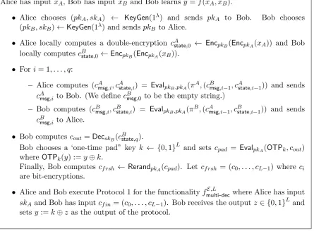
Protocol 3. General SFE Protocol for f ={fλ :{0,1}`A(λ)× {0,1}`B(λ) → {0,1}L(λ)}.
Alice has inputxA, Bob has inputxB and Bob learnsy=f(xA, xB).
• Alice chooses (pkA, skA) ← KeyGen(1λ) and sends pkA to Bob. Bob chooses
(pkB, skB)←KeyGen(1λ) and sendspkB to Alice.
• Alice locally computes a double-encryption cAstate,0 ← EncpkB(EncpkA(xA)) and Bob locally computes cB
state,0 ←EncpkB(EncpkA(xB)). • Fori= 1, . . . , q:
– Alice computes (cAmsg,i, cAstate,i) = EvalpkB,pkA(π
A,(cB
msg,i−1, cAstate,i−1)) and sends
cAmsg,i to Bob. (We definecBmsg,0 to be the empty string.)
– Bob computes (cBmsg,i, cBstate,i) = EvalpkB,pkA(π
B,(cA
msg,i−1, cBstate,i−1)) and sends
cBmsg,i to Alice.
• Bob computescout =DecskB(c
B
state,q).
Bob chooses a ‘one-time pad” key k ← {0,1}L and sets cpad = EvalpkA(OTPk, cout) whereOTPk(y) :=y⊕k.
Finally, Bob computes cf rsh ← RerandpkA(cpad). Let cf rsh = (c0, . . . , cL−1) where ci are bit-encryptions.
• Alice and Bob execute Protocol 1 for the functionalityfmulti-decE,L where Alice has input
skAand Bob has inputcf in = (c0, . . . , cL−1). Bob receives the outputz∈ {0,1}L and setsy:=k⊕z as the output of the protocol.
Figure 3: Second Construction– general protocol fory=f(xA, xB).
Theorem 3.5. Assume thatE = (KeyGen,Enc,Dec,Eval,Rerand)is an FHE scheme with reran-domization, and that the conditions of Theorem 3.3 (Protocol 1) hold. Letf be any polynomial-time functionality and let πf be any (insecure) protocol correctly evaluating f with communi-cation complexity CC(f, λ). Then Protocol 3 gives a secure SFE scheme for f. Furthermore, there is some fixed polynomial p(λ) such that for every choice of f and πf as above, the com-munication complexity of Protocol 3 is bounded by p(λ)CC(f, λ).
Proof. The communication complexity of the protocol follows by inspection.
9
We note that an alternate approach avoiding double-encryption and instead using distributed key-generation where Alice and Bob agree on a common FHE public keypkand get secret sharesskA, skB of the corresponding
To simulate an honest-but-curious Bob, the simulator runs the protocol between Alice and Bob honestly up until the last step (execution of Protocol 1) with one difference: it now computes Alice’s initial encrypted state ascAstate,0 ←EncpkB(EncpkA(0
`
A)) using a dummy value 0`A instead
of her inputxA. Finally, it simulates the execution of Protocol 1 using the one-sided simulator
for that protocol, where Bob has input cf rsh = (c0, . . . , cL−1) and output y = (y0, . . . , yL−1)∈ {0,1}L. It is clear that this is indistinguishable by the semantic security of the FHE scheme (with pkA) and the simulation-security of Protocol 1.
To simulate an honest-but-curious Alice, the simulator runs the protocol between Alice and Bob honestly up until the last step (execution of Protocol 1) with one difference: it now computes Bob’s initial encrypted state as cB
state,0 ←EncpkB(EncpkA(0
`
B)) using a dummy value
0`B instead of his input x
B. In the last step, it chooses randomnessz← {0,1}L and computes
cpad ← EncpkA(z) andcf rsh← RerandpkA(cpad). Finally, it runs a real execution of Protocol 1 between Alice and Bob where it uses the input cf rsh on behalf of Bob. Notice that in the real
protocol z = y⊕k has the same distribution as z ← {0,1}L in the simulation. Furthermore, in both the real protocol and the simulation, cf rsh is derived by running RerandpkA(cpad) on some ciphertextcpadsuch thatDecskA(cpad) =z. Therefore, the only difference between the real execution and the simulation is that (1)cBstate,0 is computed with a dummy value and (2)cpadis
computed differently but encrypts the same message. The first modification is indistinguishable by the semantic security of the FHE scheme with public key pkB. The second modification is
indistinguishable by the re-randomization security of the FHE scheme with public keypkA.
Output for Alice. Note that our positive results also extend to the case where both Alice and Bob get the same outputyor where they get different outputsyA, yBrespectively. In particular,
we can just run two sequential copies of our SFE where we reverse the roles of Alice and Bob. Using the first construction, this results in communication complexity poly(λ) +|xA|+|xB|.
Using the second construction, this results in communication complexitypoly(λ)CC(f, λ) where
CC(f, λ) is now the communication complexity of the best insecure protocol evaluatingf where both Alice and Bob get their correct outputs.
3.4 On The Necessity of Obfuscation
We show that some weak form of obfuscation is necessary to avoid “output-size dependence” for general SFE in the honest-but-curious setting. It’s not clear if this weak form of obfuscation implies iO (seems unlikely) but nevertheless it appears highly non-trivial to achieve.
Succinct Obfuscation with CRS. Consider a notion of obfuscation intended for circuits
C : [L] → {0,1} where the domain size L is some large polynomial. In other words, we would like to have an obfuscatorCe ← O(1λ,1L, C) that is allowed to run in time polynomial in the domain sizeL. This is trivial to achieve: the obfuscator just outputs Ce= [C(1), . . . , C(L)] containing the evaluation ofCon all points in its domain. Indeed, this satisfies a strong notion of black-box (BB) obfuscation where the entire obfuscated circuitCe
c
≈SC(1λ,1L) can be simulated given black-box access to C.10 Can we get such BB obfuscation scheme which is alsosuccinct, meaning that the size of the obfuscated circuit Ce is bounded by some polynomial poly(|C|, λ) independent of L? It’s easy to see that this is impossible using the same incompressibility argument as our main negative result - if the circuitC computes a PRFfk(i) fori∈[L] then a
succinct BB obfuscation scheme would need to compress the PRF outputs. Therefore, we add
one more relaxation allowing both the obfuscator and the evaluator to have access to a large common random string (CRS)r, which is chosen uniformly at random. Although the size of r
can depend on L, the size of the obfuscated circuit cannot.
Definition 3.6 (Succinct BB Obfuscation with CRS). A succinct BB obfuscator consists of a ppt obfuscator Ce ← O(1λ,1L, C, r) and a ppt evaluator b = Eval(C, i, re ), where r ←
{0,1}p(λ,L,|C|) for some polynomial p is a uniformly random CRS. For correctness, we require that for all circuits C : [L] → {0,1} and all i ∈ [L] we have Pr[Eval(O(1λ,1L, C, r), i, r) =
C(i)] = 1. For security, we require that there exists a ppt simulator S such that for any
polynomialL(λ) and any circuit ensembleC ={Cλ : [L(λ)]→ {0,1}} we have
(r,Ce)
c
≈SC(1λ,1L,|C|)
where r ← {0,1}p(λ,L,|C|),Ce ← O(1λ,1L, C, r). In other words, we can simulate the obfuscated circuit if the simulator is allowed to choose the CRS r.
Our positive result gives us such a succinct BB obfuscation scheme with a CRS using iO. To obfuscateC we first compute an SSB hashz=Hhk(r) of the CRSr and then obfuscate the circuit C[z](i, ri, πi) which verifies that ri is the correct value of the i’th bit of the pre-image
by checking the opening πi; if so, it outputs C(i). More generally, we claim that any
honest-but-curious SFE scheme with communication complexity poly(|xA|, λ) which only depends on
Alice’s input size but not Bob’s output size would give such obfuscation.
Theorem 3.7. Assume the existence of an SFE in the honest-but-curious setting for general computation y = f(xA, xB) where Bob gets the output y, and where the communication
com-plexity from Alice to Bob is bounded byp(|xA|, λ)for some fixed polynomialpindependent of the
function f or its output size L. Then there exists a succinct BB obfuscator in the CRS model, where the size of the obfuscated circuit is p(|C|, λ) independent of the domain sizeL.
Proof. Consider an SFE protocol for the functionality f(C,⊥) = y = (C(1), . . . , C(L)) where Alice gets as input some circuit C, Bob has no input, and Bob learns C(1), . . . , C(L). By as-sumption, we have an honest-but-curious SFE protocol with communication complexityp(|C|, λ) from Alice to Bob.
The CRS in the obfuscation scheme will be the randomnessrfor Bob. To obfuscate a circuit
C, the obfuscator O(1λ,1L, C, r) runs an honest copy of the SFE protocol between Alice with input C and Bob with the random coins r. It sets the obfuscated circuit Ce to consist of the protocol messages from Alice to Bob. GivenCeandr, theEvalalgorithm computes Bob’s output
y= (C(1), . . . , C(L)). The security of the obfuscation scheme follows directly from that of the SFE protocol.
It remain an interesting open problem to explore the notion of succinct BB obfuscation in the CRS further, and to see if it can be constructed under weaker assumptions than iO.
4
Lower Bounds in the Honest-But-Deterministic Setting
4.1 Yao Incompressibility Entropy
The traditional notion of Shannon entropy corresponds to how well a distribution can be com-pressed (on average). The notion of Yao incompressibility entropy [Yao82b; HLR07] extends this to the computational setting by measuring how well a distribution can be compressed when the compressor and decompressor are required to be efficient. Roughly speaking, the Yao in-compressibility entropy of a distribution X is at least k if X cannot be efficiently compressed to fewer than k bits. We will rely on a version of conditional Yao incompressibility entropy due to Hsiao, Lu and Reyzin [HLR07]. It was shown by [HLR07] that the (conditional) Yao incompressibility entropy of a distribution X is always at least as large as its HILL pseudo-entropy [HILL99], which is in turn at least as large as its min-pseudo-entropy, and the gaps between these entropies can be large. Therefore, giving a lower bound in terms of Yao entropy yields the strongest results.
Definition 4.1 (Conditional Yao Incompressibility Entropy [HLR07]). Let k = k(λ) be an integer-valued function of security parameter λ. A probability ensembleX ={Xλ}λ∈N has Yao
incompressibility entropy at least k conditioned on Z ={Zλ}λ∈N, denoted by HYao(X|Z) ≥k,
if for every pair of circuit-ensembles C ={Cλ}, D={Dλ} (called “compressor” and
“decom-pressor”) of size poly(λ) where Cλ has output-size at most k(λ)−1, there exists a negligible
functionε(·) such that
Pr (x,z)←(Xλ,Zλ)
[Dλ(Cλ(x, z), z) =x]≤
1
2 +ε(λ) .
We note that the above definition is actually somewhat weaker than the one of [HLR07]. The latter required that, if the output of the compressor has length `, then the success probability of the compressor/decompressor should be at most 2`−k+ε(λ). In our case, we only require this to hold for `= k−1. Since considering a weaker definition makes our lower bound stronger, we will use our weaker variant which is also simpler to define and use.
Letf :{0,1}`A(λ)× {0,1}`B(λ)→ {0,1}L(λ). We define the Yao incompressibility entropy of the functionf as a natural extension of the concept of the above Yao incompressibility entropy for probability ensembles (Definition 4.1). In particular, it measures the incompressibility of Bob’s output Y = f(XA, XB) conditioned on Bob’s input XB, for the choice of distributions
XA, XB which maximizes this quantity.
Definition 4.2 (Yao Incompressibility Entropy of Function). We say that a function f :
{0,1}`A(λ) × {0,1}`B(λ) → {0,1}L(λ) has Yao incompressibility entropy at least k, denoted
by k≤HYao(f), if there exist
• a probability ensembleXA={XA,λ}λ∈N of distributions over {0,1}`A(λ) and
• a probability ensembleXB={XB,λ}λ∈N of distributions over{0,1}`B(λ),
such that the ensemble Y = {Yλ}λ∈N defined via Y = f(XA, XB) satisfies k ≤ HYao(Y|XB);
i.e., the Yao incompressibility entropy of Y conditioned on XB is at least k.
4.2 Communication Complexity vs. Incompressibility Entropy
Theorem 4.3. Let f : {0,1}`A(λ)× {0,1}`B(λ) → {0,1}L(λ), and let Π = (Πoff,Πon) be an
offline/online protocol evaluatingf with one-sided security against honest-but-deterministic Bob. If the Yao incompressibility entropy of f is HYao(f) ≥ k then the communication complexity from Alice to Bob during the online phase of Π is at least k.
Proof. Assume, by contradiction, that the Yao incompressibility entropy of f is at least kbut the communication complexity from Alice to Bob during the online phase of Π is at mostk−1. Since Π securely evaluates f in the presence of honest-but-deterministic Bob (Definition 2.2), there exists an efficient simulator S = (Soff, Son) that satisfies the definition. Let X
A, XB be
distributions of Alice’s and Bob’s inputs that maximize HYao(Y|XB) where Y = f(XA, XB),
so that HYao(Y|XB) ≥ k. We show how to use the simulator S to efficiently compress the
output distributionY given XB tok−1 bits, and successfully decompress with overwhelming
probability.
Let ρ = (ρoff, ρon) be any string of random coins used by the simulator S. On input (y, xB) ← (Y, XB), the compressor Cρ runs S on (y, xB) using the randomness ρ to obtain
the simulated view (simoffB,simonB) = ((moff1 , . . . , moffs ),(xB, mon1 , . . . , mont )) of the
honest-but-deterministic adversary corrupting Bob. The compressor outputs (mon1 , . . . , mont ), i.e., the sim-ulated messages from Alice to Bob during the online phase of length at mostk−1.
On input ((mon1 , . . . , mont ), xB), the decompressorDρ runs the simulatorSoff with
random-ness ρoff to create the simulated view simoffB = (moff1 , . . . , moffs ) of the honest-but-deterministic Bob in the offline phase. The decompressor outputs the implicit output y0 of honest-but-deterministic Bob given the complete view ((moff1 , . . . , moffs ),(xB, mon1 , . . . , mont )).
Since the simulated transcript is computationally indistinguishable from the real transcript, a random compressor/decompressor pair will output a correctywith overwhelming probability, i.e., for all y, xB:
Pr
ρ[Dρ(Cρ(y, xB), xB) =y]≥1−µ(λ) ,
for a negligible µ. Hence, for all large enough λ there exists some fixed string ρλ and a pair
of circuits Cλ = Cρλ, Dλ = Dρλ of total size s(λ) ∈ poly(λ) with the output-size of Cλ being
k(λ)−1 such that
Pr
(y,xB)[Dλ(Cλ(y, xB), xB) =y]
≥1−µ(λ).
This contradicts HYao(Y|XB)≥k.
As an immediate corollary, we get that the communication complexity during the online phase must be at least as large as the output-size for any functionality with pseudorandom output. For example, we state the following for the example of PRF evaluation discussed in Section 1.1.
Corollary 4.4. Letf ={fk : {0,1}λ → {0,1}}k∈{0,1}λ be a pseudorandom function. Consider
an SFE functionality for “L PRF Evaluations” where Alice has a key k∈ {0,1}λ, Bob has no input, and Bob gets the output y = (fk(1), . . . , fk(L)) for some polynomial L = L(λ). In
any offline/online protocol Π = (Πoff,Πon) for the above functionality, with one-sided security against honest-but-deterministic Bob, the online communication from Alice to Bob must be at least L bits.
Proof. Consider the uniformly random distribution of Alice’s input k. Then Bob’s output
y = (fk(1), . . . , fk(L)) is pseudorandom and therefore the HILL and Yao incompressibility
Extension to Multi-Party SFE. Our negative results also extend to multi-party SFE. In particular, for an n-party functionality (y1, . . . , yn) = f(x1, . . . , xn) where party Pi has input
xi and output yi, we can define the i’th output entropy off as being at least k if there exists
some distribution (X1, . . . , Xn) such that HYao(Yi|Xi) ≥k where Y =f(X1, . . . , Xn). In that
case, in any offline/online n-party SFE protocol that has one-sided security against a single honest-but-deterministic party Pi, the communication-complexity from all other parties to Pi
must be at leastk bits. This simply follows by thinking of partyPi as Bob and thinking of all
of the other parties as Alice in a two-party SFE protocol.
4.3 Application: Lower Bounds for Functional Encryption
The impossibility of functional encryption with simulation based security for general circuits was first shown by Agrawal et al. [AGVW13]. This result was later extended to prove lower bounds for various related notions of functional encryption [DIJ+13; DI13; GGJS13]. In this section we show that the above lower bounds for functional encryption follow from our lower bound on communication complexity in offline/online SFE secure against honest-but-deterministic Bob.
Definition 4.5 (Functional Encryption). Let C = {Cλ}λ∈N be a function family, where each
circuitC ∈ Cλ takes as input a stringx∈ {0,1}m(λ)and outputsC(x)∈ {0,1}. Afunctional en-cryption schemeF E for a circuit familyCconsists of four algorithmsF E = (Setup,KeyGen,Enc,Dec)
defined as follows:
• F E.Setup(1λ) is appt algorithm that takes as input the unary representation of the
secu-rity parameter and outputs the master public and secret keys (MPK,MSK).
• F E.KeyGen(MSK, C) is a ppt algorithm that takes as input the master secret key MSK
and a circuit C ∈ Cλ and outputs a corresponding secret keyskC.
• F E.Enc(MPK, x) is a ppt algorithm that takes as input the master public key MPK and
an input message x∈ {0,1}m(λ) and outputs a ciphertext c.
• F E.Dec(skC, c) is a deterministic algorithm that takes as input the secret key skC and a
ciphertextc and outputs y.
We require:
Correctness: For all C ∈ Cλ and all x∈ {0,1}m(λ),
Pr
y 6=C(x)
(MPK,MSK)← F E.Setup(1λ),sk
C ← F E.KeyGen(MSK, C),
c← F E.Enc(MPK, x), y ← F E.Dec(skC, c)
=negl(λ) ,
where the probability is taken over the coins of F E.Setup, F E.KeyGen, and F E.Enc.
L-SIM Security: For security, we require that there exists a simulator S = (S1, S2) such that
for every choice of the circuits C1, . . . , CL∈ Cλ and every x∈ {0,1}m(λ) we have
( view1 = (MPK,skC1, . . . ,skCL) , view2=c )
c
≈ ( sim1 , sim2 )
where (MPK,MSK)← F E.Setup(1λ), skCi ← F E.KeyGen(MSK, Ci), c← F E.Enc(MPK, x)
and (sim1,state)←S1(1λ, C1, . . . , CL), sim2 ←S2(C1(x), . . . , CL(x),state).