Application of Multi Network Alignment Algorithms
for Connectomes Study
Marianna Milano1,‡, Pietro Hiram Guzzi1,‡* and Mario Cannataro1
1 Department of Surgical and Medical Sciences, University of Catanzaro; m.milano,hguzzi,[email protected]
* Correspondence: [email protected]
‡ These authors contributed equally to this work.
Abstract: A growing area in neurosciences is focused on the modeling and analysis the complex 1
system of connections in neural systems, i.e. the connectome. Here we focus on the representation of 2
connectomes by using graph theory formalisms. The human brain connectomes are usually derived 3
from neuroimages; the analyzed brains are co-registered in the image domain and brought to a 4
common anatomical space. An atlas is then applied in order to define anatomically meaningful 5
regions that will serve as the nodes of the network - this process is referred to as parcellation. Recently, 6
it has been proposed to perform atlas-free random brain parcellation into nodes and align brains in 7
the network space instead of the anatomical image space to define network nodes of individual brain 8
networks. In the network domain, the question of comparison of the structure of networks arises. 9
Such question is tackled by modeling the comparison of brain network as a network alignment (NA) 10
problem. In this paper, we first defined the NA problem formally, then we applied three existing state 11
of the art of multiple alignment algorithms (MNA) on diffusion MRI-derived brain networks and we 12
compared the performances. The results confirm that MNA algorithms may be applied in cases of 13
atlas-free parcellation for a fully network-driven comparison of connectomes. 14
Keywords:graph alignment; brain network; human connectome 15
1. Introduction 16
The human brain is a complex organ organized into a dense system of connections, also known as 17
connectome. Recent studies have shown that this system of connections is responsible for the brain 18
activity, and an alteration of connections (decreased or increased connectivity) can led to the insurgence 19
of neurological diseases [1,2]. For this reasons, many researches in neuroscience have been focused 20
on mapping and analysis of the human brain connectome [3]. Connectome may be analyzed using 21
different zoom, e.g. by focusing on single components, i.e. neurons and axons, or grouping them into 22
regions. Usually the analysis of single components is defined to as anatomic connectivity, while the 23
analysis of regions is called functional connectivity because regions are in general perfoming different 24
functions. Tipically, the human brain connectome can be mapped using neuroimaging techniques, 25
such as Magnetic Resonance Imaging (MRI), Electroencephalography (EEG), and Electromyography 26
(MEG) enabling to take a picture of the brain connections of patients [4]. Among the others, the main 27
source for deriving information about connectomes is Magnetic Resonance Imaging (MRI) [5] able to 28
achieve both informations about anatomic connectivity and functional connectivity. 29
Once obtained, the connectome data need to be characterized through sophisticated analytic 30
strategies. A useful strategy is based on graph theory [6], that ensures the modeling of such data 31
into a network model. Different studies have used the network models to extract clinically relevant 32
information [7,8] due to the capability to summarize the characteristics of a complex network with 33
few measures and to understand the organization of both entire networks and individual network 34
elements [6]. 35
Graph theoretical approaches model the human brain as set of nodes linked by edges. The 36
nodes typically represent region of interest (ROI) and the edges represent functional or anatomical 37
connections. A typical MRI experiment produces a series of images, either from intra-subject or 38
inter-subject, then the MRI images are modeled as networks. A further step consists of the coregistration 39
among the network and a brain atlas in order to obtain anatomically meaningful regions [9]. Recently, 40
Tymofiyeva et al. [10] proposed an alternative method based on the application of atlas-free parcellation 41
and on the construction of individual connectomes only in the network space. In the network domain, 42
an appropriate analytic strategy consists of the comparison of studied networks by recurring to 43
network alignment (NA) approaches. The techniques for the alignment of biological networks fall into 44
sub-categories: local alignment, to find small conserved motifs across networks, and global alignment, 45
which attempts to find a best mapping between all nodes of the two networks or pairwise alignment 46
to align two networks and multiple alignment that align multiple networks. Different studies have 47
widely usad the NA approaches for the analysis of biological networks. In previous works [11,12] we 48
explored the possibility to apply the NA methods for the analysis of to MRI connectomics. At first we 49
tested different global alignment algorithms to build the alignments among the diffusion MRI-derived 50
brain networks. Then, we analyzed the alignment results in term of topological quality measures 51
and according to these analyses, we identified the best alignment algorithm to align the diffusion 52
MRI-derived brain networks. However, recent studies have demonstrated in an independent way 53
that the multiple alignment algorithms are able to exact deeper information than pairwise alignment 54
algorithm when these one are applied to molecular biology analysis [13]. 55
According to these studies, we choose to apply multiple alignment algorithms on MRI 56
connectomics. Here, we selected three existing state of the art multiple alignment algorithms to 57
build the alignment of diffusion MRI-derived brain networks. The algorithms tested here are 58
MultiMAGNA++ [13], GEDEVO-M [14] and IsoRankN [15]. The algorithms are applied to build 59
the multiple alignment among the diffusion MRI-derived brain networks. After the alignments were 60
built, we compared the performance of these algorithms. 61
2. Methodology for Brain Network Analysis 62
In this section, we present the workflow of analysis that can be preformed on the brain network 63
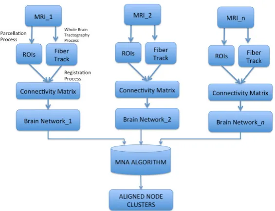
starting from the building of connectome from MRI images. The Figure1shows a workflow of 64
Methodology for the Brain Network Analysis from the building of representative network from 65
experimental data to the comparison of brain network applying multiple alignment algorithm. 66
2.1. Building a Brain Network 67
The building of brain network starts with a set of anatomical or physiological observations [16], 68
then the structural and functional connectivity data are processed into network model exploiting graph 69
theory. 70
However, the application of graph theory to the study of connectomes presents some challenges 71
related to the description of nodes and edges [17]. For example, an ideal definition of nodes should 72
group a set of neurons according to maximal functional homogeneity within nodes and the maximal 73
functional heterogeneity among different nodes. According to this, there is no clear evidence for the 74
optimal definition of both nodes and edges. A common approach to define the nodes of a brain network 75
consists of the subdivision of the brain into homogeneous, non-overlapping and large-scale, regions 76
respect to information provided, generally, by techniques based on magnetic resonance imaging (MRI) 77
[18], also known as “parcellation process”. Especially, MRI has allowed to obtain information about 78
anatomical connectivity, functional connectivity, or task-related activation. 79
Currently, there exist three different approaches applied to parcellation of connectome: 80
1. Parcellation of the brain by using predefined anatomical templates that consists of the 81
Figure 1.Building a representative network from experimental data: example of a workflow. Diffusion or functional MRI images are acquired for a subject according to the study to be conducted. The MRIs are used to perform whole-brain parcellation by selecting a suitable method. Starting from the parcelled whole brain the computation of connections is performed the connectivity matrix is constructed. Then, the resulting brain network is obtained. This process is preformed for each studied subject. A MNA algorithms takes as input the brain networks and produces aligned node clusters between more than two networks.
areas [19]. This approach enables to subdivide the whole brain into labeled regions according to 83
the different labels regions of the templates; 84
2. Parcellation of the brain by usingrandomly generated templates[20] that ensures to divide the 85
whole brain into parcels (brain region) of roughly equal size; 86
3. Connectivity-based parcellationsthat aim to delineate brain regions according to the similarities 87
in structural or functional connectivity patterns. 88
Due to the different approach, the choice of a parcellation scheme is fundamental for subsequent 89
analysis on brain network. In fact, each parcellation method presents some pitfalls. 90
For example, the parcellation of the brain by using predefined anatomical template raises the 91
question of the accuracy of mapping. Since atlas based on the Brodmann areas are originally defined 92
using cytoarchitectural differences between brain regions, in the registration step a mismatch among 93
the cortical surface analyzed and the borders of the Brodmann areas may occurs [10].Thus, this 94
approach is limited by inter-subject variability and can be especially problematic in the context of brain 95
maturation. In this paper, we focus on the random, atlas-free definition of nodes in individual subjects 96
(see [12] for a deep description), which can allow for a fully network-driven way of looking at the 97
brain and comparing brains of different subjects and, potentially, species [10]. 98
The definition of the edges is also currently an open challenge related to a) the type of connectivity 99
measured, and b) the method used to quantify it. As mentioned above, brain connectivity can refer 100
to different aspects of brain organization including (i)anatomical connectivityconsisting of axonal 101
fibers connecting cortical and subcortical regions inferred from diffusion imaging, and (ii)functional 102
connectivitydefined as the observed statistical correlations of the BOLD signal between brain regions. 103
Once the nodes and the edges are defined, the pattern of connections between brain regions 104
(nodes) can be stored into the Connectivity Matrix [21]. The Connectivity Matrix is symmetric matrix 105
(edge) between the regions. This representation lends itself to be mapped to a graphical model which 107
ensures to quantify different topological aspects of the connectome. 108
2.2. Comparison of Brain Network: Network Alignment 109
A crucial point in the connectome analysis regards the comparison of the brain networks. Thus, 110
the detection of an correct node mapping between atlas-free networks may uncover significant aspcets 111
on the comparison of brains or structure of groups of subjects, such as healthy versus diseased subjects. 112
Many different network alignment methods have been proposed in biological fields [22]. 113
Formally, a graph G is defined asG={V,E}, where V is a finite set of nodes and E is a finite set of 114
edges. LetG1={V1,E1}andG2={V2,E2}be two graphs, whereV1,2are sets of nodes andE1,2are sets 115
of edges, a graph alignment is the mapping between the nodes of the input networks that maximizes 116
the similarity between mapped entities. From a theoretical point of view, the graph alignment problem 117
consists of finding an alignment function (or a mapping) f :V1→V2that maximizes a cost function 118
Q. The similarity between the graphs is defined by a cost function,Q(G1,G2,f), also known as the 119
quality of the alignment. Let f be an alignment between two graphsG1andG2, given a nodeufrom 120
G1, f(u)is the set of nodes fromG2that are aligned under f tou. Q expresses the similarity among 121
two input graphs with respect to a specific alignment f and the formulation of Q strongly influences 122
the mapping strategy. 123
There exist different formulations of Q that fall into following the classes: 124
Topological Similarity: Graphs are aligned by considering only edge topology, so that the perfect 125
alignment is reached when input graphs are isomorphic. 126
Node Similarity: Such function considers the similarity among mapped nodes. Nodes of the 127
aligned graphs can be more or less similar to each other. Thus the alignment should align each node of 128
one graph to the most similar node of the other one given a node similarity functions,s(v1,v2)→R, 129
v1∈V1,v2∈V2. 130
Hybrid approaches: Some recent formulations of Q take into account of both of the approaches 131
by linear combination. 132
The network alignment problem can be formulated according to: i) the kind of input,pairwise or 133
multiple alignmentand ii) the scope of node mapping required,local or global alignment. In general, the 134
network alignment can be classified as local alignment or global alignment. Thelocal alignmenttypically 135
finds multiple and unrelated regions of isomorphism among the input networks, each region implying 136
a mapping independently of the others. Therefore, the computed correspondences may involve 137
overlapping subgraphs. The output of local network alignment is a set of pairs of possibly overlapping 138
subgraphs of the input networks. The literature contains many algorithms that address local graph 139
alignment problem. For example, AlignNemo [23] and AlignMCL [24] algorithms. Theglobal alignment 140
aims to find a mapping that should cover all of the nodes of the input networks. Global alignment 141
returns a unique overall alignment between the input networks, such that a one-to-one correspondence 142
is found between of a network with one node of the other network. Most popular existing methods of 143
global alignment are MAGNA [25], NETAL [26], GHOST [27], WAVE [28]. For a complete review on 144
global and local network alignment algorithms and their advantages or disadvantages see [29]. 145
Also, the network alignment methods can bepairwise or multiple alignment. 146
The pairwise network alignment (PNA) aligns two networks at a time and produces aligned node 147
pairs between two networks. The multiple network alignment (MNA) aligns three or more networks 148
to each other at once and produces aligned node clusters. PNA and MNA can be local or global, with 149
one-to-one or many-to-many node mappings. The difference between one-to-one and many-to-many 150
mapping in the pairwise alignment refers the previous discussion on global and local alignment. The 151
PNA can search the similar small subnetworks exploiting many-to-many mapping between nodes of 152
the compared network or can look for the best overlap of the whole compared networks exploiting 153
containing at most one node per network, whereas MNAs are many-to-many MNA methods when an 155
aligned cluster contains more than one node from a single network. 156
In literature, both PNA and MNA are applied to built the alignment protein interaction networks 157
(PINs) [30]. Since, MNA can capture functional knowledge that is common to multiple species, 158
it was detected that MNA leads to deeper biological information than PNA. However, MNA is 159
computationally much harder than PNA because the complexity of the network alignment problem 160
increases exponentially with the number of analyzed networks. 161
There exist different proposed multiple network alignment algorithms in literature such as 162
MultiMAGNA++ [13], GEDEVO-M [14] and IsoRankN [15]. 163
In this work, three multiple alignment algorithms were chosen to built the multiple alignment of 164
brain networks. We give hereafter a short conceptual description. 165
A popular existing method of multiple alignment is MultiMAGNA++ [13]. MultiMAGNA++ is a 166
a global one-to-one MNA aligner that simulates a population of alignments that evolves over time 167
by applying a genetic algorithm and a function for the crossover of two alignments into a superior 168
alignment. Since the genetic algorithm simulates the evolutionary process guided by the survival 169
of the fittest principle, only alignments, i.e. those that conserve the most edges, survive. Thus, 170
MultiMAGNA++ proceeds to the next generation, until the alignment accuracy cannot be optimized 171
further. 172
The second multiple aligner is GEDEVO-M [14] a global one-to-one MNA aligner. GEDEVO-M is 173
an extension of GEDEVO [31] tool for efficient global graph alignment. Underlying the GEDEVO-M 174
method is the Graph Edit Distance model (GED), where a graph is transferred into another one with a 175
minimal number of edge insertions and deletions. Thus, GEDEVO-M uses the GED as optimization 176
model for finding the best alignments and then minimizes the sum of GEDs between every pair of 177
input networks. 178
The last multiple aligner is IsoRankN [15], a global many-to-many MNA alignment tool based a 179
spectral clustering method to find dense and clique modules when the global alignment of multiple 180
networks is computed. 181
3. Results 182
3.1. Dataset 183
The dataset consisted of 24 diffusion MRI-derived structural networks of human brain: 12 184
networks with a number of nodes equal to 95 and the 12 networks with a number of nodes equal to 185
1000. The brain networks are related to three different stages of development by including newborns 186
(NE), six-month-old infants (6M), and adults (AD). SeeMaterials and Methods Sectionfor a complete 187
description. 188
3.2. Building of brain network multiple alignment 189
We built the multiple alignment of all networks with 95 and 1000 nodes (for convenience we call 190
the two datasetnetworks95andnetworks1000) related to same growth stages (NE, 6M, AD) by applying 191
MultiMAGNA++ [13], GEDEVO-M [14] and IsoRankN [15]. 192
We ran all MNA methods on the same Linux machine with Intel Core i5 and 4GB of RAM. We 193
selected the following MultiMAGNA++ parameters: CIQas measure of Edge Conservation, theα
194
parameter equal to 0, in order to consider only topology, whereas the population size, number of 195
generation, fraction of elite members were set to default values. We tested different parameters and 196
obtained best results with the default parameters for GEDEVO-M:popparameter that controls the 197
number of new individuals per iteration set equal to 1000 andmaxsamethat controls the stop after N 198
iterations without any score improvement were equal to 3000. To build the multiple alignment with 199
IsoRankN we set: the max number of iterationsKequals to 30, the thresholdthreshequals to 1e−4, 200
maxveclenequals to 1000000 and theαparameter equal to 1 in order to consider only network data.
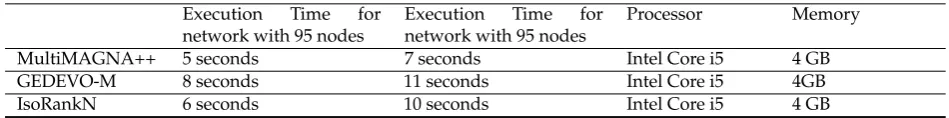
The Table1reports the execution time of MultiMAGNA++, GEDEVO-M and IsoRankN to build the 202
multiple alignment on the networks with 95 nodes and on the networks with 1000 nodes. 203
Table 1. Execution Time to build the multiple alignment with MultiMAGNA++, GEDEVO-M and IsoRankN for the networks with 95 nodes and the networks with 1000 nodes
Execution Time for network with 95 nodes
Execution Time for network with 95 nodes
Processor Memory
MultiMAGNA++ 5 seconds 7 seconds Intel Core i5 4 GB
GEDEVO-M 8 seconds 11 seconds Intel Core i5 4GB
IsoRankN 6 seconds 10 seconds Intel Core i5 4 GB
3.3. Topological alignment quality evaluation 204
Here, we aim to evaluate the quality of the multiple alignments built with MultiMAGNA++, 205
GEDEVO-M and IsoRankN algorithms. The topological quality is related to two alignment algorithm 206
capability as the reconstruction of the true node mapping and the conservation of as much as possible 207
edges. Typically, the Node Correctness (NC) is the measure widely used to evaluate how an alignment 208
reconstructs the true node mapping correctly. Instead, different measures are used to evaluate how 209
well the edges are conserved on an alignment, such as EC, ICS orS3(see the previous Section). In 210
general, the Edge Correctness is defined as the number of edges conserved under an alignment f with 211
respect to the total number of edges of input networks. Thus, once the multiple alignments were built, 212
we performed an evaluation of alignment quality by comparing the Edge Correctness (EC) [25] related 213
to the alignments built with MultiMAGNA++, GEDEVO-M and IsoRankN. 214
The Table2and Table3report the global Edge Correctness computed on the multiple alignment 215
of all networks with 95 nodes and with 1000 nodes related to same growth stages NE, 6M, AD by 216
applying MultiMAGNA++, GEDEVO-M and IsoRankN algorithms. 217
Table 2. Comparison the Edge Correctness of the multiple alignments built with MultiMAGNA++, GEDEVO-M and IsoRankN.
Edge Correctness NE 6M AD
MultiMAGNA++ 0.5 0.55 0.49
GEDEVO-M 0.441 0.441 0.48
IsoRankN 0.477 0.477 0.485
Table 3. Comparison the Edge Correctness of the multiple alignments built with MultiMAGNA++, GEDEVO-M and IsoRankN.
Edge Correctness NE 6M AD
MultiMAGNA++ 0.14 0.16 0.19
GEDEVO-M 0.089 0.091 0.099
IsoRankN 0.095 0.099 0.1
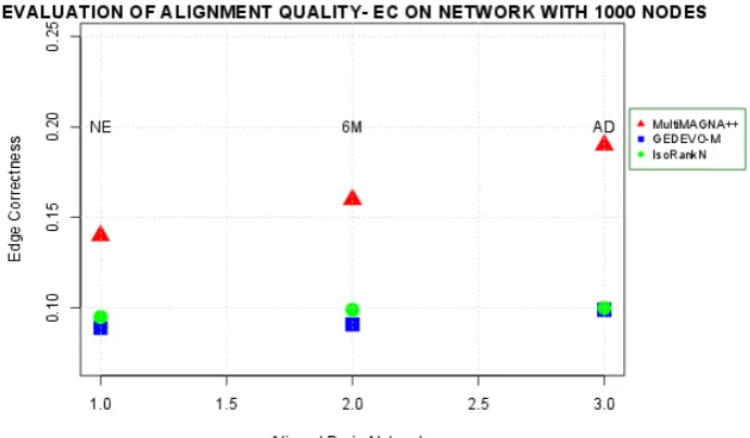
Figure2shows an overview of edge conservation comparison onnetworks95 whereas Figure 218
3 shows an overview of edge conservation comparison on networks1000. We note that the best 219
results in terms of edge conservation were obtained when applying MultiMAGNA++ as global 220
aligner both onnetworks95 andnetworks1000. In fact, the mean edge correctness values are higher 221
on the alignments built with MultiMAGNA++ than mean edge correctness scores on alignments 222
obtained with GEDEVO-M and IsoRankN. The reason is related to the strategy of MultiMAGNA++ to 223
construct the multiple alignment. In fact, MultiMAGNA++ is the unique multiple aligner that directly 224
optimizes edge conservation in addition to node conservation by using a genetic algorithm, whereas 225
MultiMAGNA++ results improved. This entails an inferior behavior of GEDEVO-M and IsoRankN 227
compared to the MultiMAGNA++. 228
We also note that values of EC fornetworks95are higher than EC fornetworks1000. 229
Figure 2. The topological evaluation of alignments built with MultiMAGNA++ (red marker), GEDEVO-M (blue marker), IsoRankN (green marker). The Figure shows the mean Edge Correctness scores of alignments built among the networks with 95 nodes by applying the selected three multiple aligners.
4. Discussion 230
The brain connectivity refers to different aspects of brain organization including i) anatomical 231
connectivity consisting of axonal fibers across cortical regions and ii) functional connectivity defined 232
as the observed statistical correlations of the BOLD signal between regions of interest. Understanding 233
brain connectivity can shed light on the brain cognitive functioning that occurs via the connections 234
and interaction between neurons. Brain connectivity can be modeled and quantified with a large 235
number of techniques. A useful formalism to represent the brain connectivity derives from graph 236
theory. The graph theoretical modeling of the human connectome has enabled important discoveries 237
by comparing the brain networks of studied subjects. In this study we proposed to apply three multiple 238
alignment algorithms MultiMAGNA++, GEDEVO-M and IsoRankN to align atlas-free human brain 239
networks at three developmental stages. We decided to apply MNA algorithms to the study of brain 240
networks because, in previous studies conducted on PINs, MNA were able to lead to deeper biological 241
compared to PNA, by capturing conserved network regions between multiple networks. We analyzed 242
the multiple alignment results in term of topological quality measures, by comparing the EC related to 243
each alignment. According to these analyses, MultiMAGNA++ resulted in the best alignment. The 244
reason is related to the strategy underlying MultiMAGNA++ to construct the multiple alignment 245
by optimizing simultaneously the edge conservation and node conservation. Our ongoing study is 246
focused on the implementation of an ad hoc algorithm for connectome alignment. Since there are 247
many conditions in which the classical parcellation is not useful, we retain that this seminal work may 248
Figure 3. The topological evaluation of alignments built with MultiMAGNA++ (red marker), GEDEVO-M (blue marker), IsoRankN (green marker). The Figure shows the mean Edge Correctness scores of alignments built among the networks with 1000 nodes by applying the selected three multiple aligners.
5. Materials and Methods 250
5.1. Dataset 251
The dataset consisted of diffusion MRI-derived structural networks of human brain at different 252
stages of development, starting with neonates [10]. Acquisition of the MRI data was compliant with 253
the Health Insurance Portability and Accountability Act (HIPAA) and the study was approved by 254
the Committee on Human Research (CHR) of the University of California, San Francisco. Three age 255
groups were included: 4 neonates imaged in the first 4-5 days of life (NE), 4 six-month-old infants 256
(6M), and 4 adults (age 24-31 years) (AD). The two pediatric groups had transient encephalopathy 257
at birth, but none of the patients had clinical or imaging evidence of brain injury. The subjects were 258
scanned on a 3T GE MR scanner using a spin echo (SE) echo planar imaging (EPI) diffusion tensor 259
imaging DTI sequence with parameter described in [10]. Tensor calculation, tractography, cortical 260
parcellation into N equal-area nodes (Figure??), and construction of the connectivity matrices was 261
performed as described previously [10]. All networks were binarized with a threshold of 1 streamline. 262
Starting from the images we obtained two different datasets. The first dataset consist of 12 networks 263
with number of nodes equal to 95 depending on parcellation step. For convenience we call this dataset 264
networks95. Table4shows the networks parameters. About the second dataset, the 12 networks were 265
constructed by setting the number of equal-area nodes for the cortical parcellation equal to 1000. Since 266
all cortical areas of the brain are connected, a fine parcellation should ensure the interconnectedness of 267
the whole brain, leaving no nodes isolated. In [10] the authors demonstrated that the highest number 268
of nodes at which this condition is fulfilled in equal to 95. For this reason, the networks of the second 269
dataset showed the isolated nodes that were not computed in the construction of the connectivity 270
matrices. For convenience we call this datasetnetworks1000even though the nodes number is different 271
Table 4.Details of brain networks with 95 nodes used for experiments
Network Nodes Edge
NE01 95 341
NE02 95 341
NE03 95 334
NE04 95 320
6M01 95 353
6M02 95 333
6M03 95 333
6M04 95 338
AD1 95 449
AD2 95 406
AD3 95 438
AD4 95 416
Table 5.Details of brain networks with 1000 nodes used for experiments
Network Nodes Edge
NE01 889 2555
NE02 904 2618
NE03 900 2585
NE04 899 2298
6M01 902 2458
6M02 849 2182
6M03 805 1928
6M04 851 2087
AD1 902 3146
AD2 869 2691
AD3 878 3262
AD4 853 2907
5.2. Alignment Algorithms 273
In this section we describe in detail the multiple alignment algorithms selected to align the 274
diffusion brain networks. 275
MultiMAGNA++ [13] is a global one-to-one MNA algorithm based on a genetic algorithm to 276
build an improved alignment. By simulating the evolutionary process, guided by the survival of 277
the fittest principle, the genetic algorithm directly optimizes both edge and node conservation while 278
the alignment is constructed. In details, MultiMAGNA++ uses the genetic algorithm to simulates a 279
population of alignments that evolves over time and then applies new function for the crossover of 280
parent alignments into a superior child alignment that allows for aligning multiple networks. 281
The genetic algorithm requires an initial population of a given number of members. In 282
MultiMAGNA++, the members of population are multiple alignments. A multiple network alignment 283
(MNA) ofknetworks, ordered in terms of the number of nodes from the smallest to the largest one, 284
is represented by usingk−1 permutations which are bijective mappings between pairs of networks 285
adjacent. The permutations are set of disjoint node clusters that cover nodes in theknetworks. So 286
MNA can be defined as multi permutation. The members of a population crossover with each other to 287
produce new members. Only the fitted members are more likely to crossover. Thus, the child alignment 288
resulting from a crossover function reflects each parent. In MultiMAGNA++, the crossover function is 289
defined as the midpoint of the shortest path between two permutations. In this way, the child MNA 290
shares the characteristics of each of the two parent MNAs. To avoid the size of the population to grow 291
without bound, the size is kept constant across all generations, with only the fittest members surviving 292
from one generation to the next. The fitness function is a combined measure of edge conservationSE 293
αSE+ (1−α)SN (1)
whereαcontrols the contribution of each node and edge conservation measures and takes the
295
values between 0 and 1. 296
The edge conservation measure used in MNA is Conserved Interaction Quality (CIQ). CIQ is a weighted sum of edge conservation between all pairs of alignedaandbclusters and is defined as:
SE=CIQ= ∑a,b
|Ea,b|cs(a,b)
∑a,b|Ea,b| (2)
where,|Ea,b|is the number of edges that connect the clusters, andcs(a,b)is edge conservation 297
between two clusters. Letr(a,b)be the number of networks that the edges which connect the clusters 298
belong to ands(a,b)be the number of networks that contain at least one node in both clusters,cs(a,b) 299
is equal to 0 ifr(a,b)≤1, alsocs(a,b)is equal tors((a,ba,b)). 300
The node conservation measure for MNA refers to internal cluster quality, i.e, the nodes in each cluster should be highly similar to each other with respect to some node cost function.
SN=
1 n∑
n i=1(|ai1|
2)
∑(u,v)∈P(ai)s(u,v) (3)
wheres(u,v)is the similarity between nodesuandvwith respect to some node cost function,ai 301
is a aligned clusters withi=1, ...,n,|ai|is the size ofaiandP(ai)is the set of all pairs of nodes inai. 302
The genetic algorithm produces newer generations until the alignment quality cannot be 303
optimized further. 304
GEDEVO-M [14] is a global one-to-one MNA algorithm based on an evolutionary algorithm that 305
uses the Graph Edit Distance (GED) as optimization model for finding the best alignments. The GED 306
is defined as the minimum insertions and deletions of edges required to transfer a graph into another 307
graph. GEDEVO-M applies the Graph Edit Distance to multiple graph models and considers the 308
alignment building as Topological Multiple one-to-one Network Alignment (TMNA). TMNA problem 309
aims to find a multiple mappingFon a set of graphsG, such that the multiple Graph Edit Distance 310
mGEDF is minimal over all possible multiple mapping onG. By minimizing themGEDF, the number 311
of edges that are aligned in multiple networks simultaneously is maximized. The GEDEVO-M builds 312
the alignment by generating an initial multiple mapping with random permutations. A one-to-one 313
MNA ofGgraphs consists of a set of disjoint clusters. Each cluster can be represented as a tuple. 314
Initially, GEDEVO-M fixes a threshold, defined as the average over all tuple scores and then it randomly 315
swaps the tuples that have scores higher than the threshold. The tuples with lower than the threshold 316
are also given a certain chance to be swapped. After that, GEDEVO-M uses a crossover operator to 317
construct a new multiple mapping from two or more parent individuals of the previous generation. At 318
first, GEDEVO-M computes the tuple scores for every possible subset ofG. Then, GEDEVO-M iterates 319
over the corresponding tuple scores by starting with larger subsets ofGand assigns some of these 320
tuples to a new multiple mapping until every subset is considered. Finally, GEDEVO-M evaluates the 321
quality of the multiple mapping by using the scoreS. The scoreSdepend on the multiple Graph Edit 322
Distance (mGED) and Graphlet-degree signature distance (GSD) of multiple mapping that computes 323
the difference in neighboring topologies of potentially matched nodes. 324
IsoRankN [15] is a global many-to-many MNA alignment tool based a spectral partitioning 325
method to find dense and clique clusters on multiple-network alignment. 326
IsoRankN builds a multiple network alignment by local partitioning the graph of pairwise 327
functional similarity scores. Initially, IsoRankN computes the functional similarity scores of every pair 328
of nodes ofknetworks. In this way, a functional similarity graph, where each edge is weighted by its 329
functional similarity score, is obtained. Then, IsoRankN applies a star spread method on functional 330
for each node, every neighbor connected with an edge whose weight is greater than a threshold; this 332
represent the star of a nodeS. 333
Then, IsoRankN orders the nodes according to the total weight of the starS. For each the starS, a 334
subset with highly weighted neighborhood is found. This subset represents a functionally conserved 335
interaction cluster. Finally, IsoRankN performed a merging stars process, by looking at the neighbors 336
of the neighbors of a node and by merging the stars of two nodes if every member of star related to a 337
node 1 has the node 2 as a neighbor and vice versa. The process is repeated until all nodes are assigned 338
to a cluster. 339
Acknowledgments: PHG,MM and MC have been partially supported by the following research project 340
funded by the Italian Ministry of Education and Research (MIUR): BA2Know-Business Analytics to Know 341
(PON03PE_00001_1). The authors wish to thank Olga Tymofiyeva for her suggestions to this research activity. 342
Author Contributions: PHG and MM conceived the main idea of the algorithm and designed the tests. MC 343
supervised the design of the algorithm. PHG and MM designed the functional requirements of the software tool. 344
All authors read and approved the final manuscript. 345
Conflicts of Interest:The authors declare no conflict of interest. 346
Abbreviations 347
The following abbreviations are used in this manuscript: 348
349
NA Network Alignment
PNA Pairwise Network Alignment MNA Multiple Network Alignment MRI Magnetic Resonance Imaging ROIs Region of Interest
DTI Diffusion Tensor Imaging PINs Protein Interaction Networks BOLD Blood Oxygenation Level Dependent
NE Newborns
6M Six-Month-Old
AD Adults
HIPAA Health Insurance Portability and Accountability Act CHR Committee on Human Research
S3 Symmetric Substructure Score EC Edge Correctness
SE Edge Conservation SN Node Conservation
CIQ Conserved Interaction Quality GED Graph Edit Distance
TMNA Multiple one-to-one Network Alignment mGEDF Multiple Graph Edit Distance
350
References 351
1. Kiani, R.; Cueva, C.J.; Reppas, J.B.; Peixoto, D.; Ryu, S.I.; Newsome, W.T. Natural grouping of neural 352
responses reveals spatially segregated clusters in prearcuate cortex. Neuron2015,85, 1359–1373. 353
2. Bargmann, C.I.; Marder, E. From the connectome to brain function. Nature methods2013,10, 483–490. 354
3. Sporns, O.; Tononi, G.; Kötter, R. The human connectome: a structural description of the human brain. 355
PLoS Comput Biol2005,1, e42. 356
4. Xia, M.; He, Y. Magnetic resonance imaging and graph theoretical analysis of complex brain networks in 357
neuropsychiatric disorders.Brain connectivity2011,1, 349–365. 358
5. Toga, A.W.; Clark, K.A.; Thompson, P.M.; Shattuck, D.W.; Van Horn, J.D. Mapping the human connectome. 359
6. Bullmore, E.; Sporns, O. Complex brain networks: graph theoretical analysis of structural and functional 361
systems.Nature Reviews Neuroscience2009,10, 186–198. 362
7. Cannataro, M.; Guzzi, P.H.; Veltri, P. Protein-to-protein interactions: Technologies, databases, and 363
algorithms. ACM Computing Surveys (CSUR)2010,43, 1. 364
8. Lesne, A. Complex Networks: from Graph Theory to Biology. Letters in Mathematical Physics2006, 365
78, 235–262. 366
9. Yap, P.T.; Wu, G.; Shen, D. Human Brain Connectomics: Networks, Techniques, and Applications [Life 367
Sciences]. IEEE Signal Processing Magazine2010,27, 131–134. 368
10. Tymofiyeva, O.; Ziv, E.; Barkovich, A.J.; Hess, C.P.; Xu, D. Brain without anatomy: construction and 369
comparison of fully network-driven structural MRI connectomes. PloS one2014,9, e96196. 370
11. Milano, M.; Tymofiyeva, O.; Xu, D.; Hess, C.; Cannataro, M.; Guzzi, P.H. Using Network Alignment for 371
Analysis of Connectomes: Experiences from a Clinical Dataset. Proceedings of the 7th ACM International 372
Conference on Bioinformatics, Computational Biology, and Health Informatics. ACM, 2016, pp. 649–656. 373
12. Milano, M.; Guzzi, P.H.; Tymofieva, O.; Xu, D.; Hess, C.; Veltri, P.; Cannataro, M. An extensive assessment 374
of network alignment algorithms for comparison of brain connectomes. BMC bioinformatics2017,18, 235. 375
13. Vijayan, V.; Milenkovic, T. Multiple network alignment via multiMAGNA++. arXiv preprint 376
arXiv:1604.017402016. 377
14. Ibragimov, R.; Malek, M.; Baumbach, J.; Guo, J. Multiple graph edit distance: simultaneous topological 378
alignment of multiple protein-protein interaction networks with an evolutionary algorithm. Proceedings 379
of the 2014 Annual Conference on Genetic and Evolutionary Computation. ACM, 2014, pp. 277–284. 380
15. Liao, C.S.; Lu, K.; Baym, M.; Singh, R.; Berger, B. IsoRankN: spectral methods for global alignment of 381
multiple protein networks. Bioinformatics2009,25, i253–i258. 382
16. Sporns, O.Networks of the Brain; MIT press, 2010. 383
17. Fornito, A.; Zalesky, A.; Breakspear, M. Graph analysis of the human connectome: promise, progress, and 384
pitfalls. Neuroimage2013,80, 426–444. 385
18. Thirion, B.; Varoquaux, G.; Dohmatob, E.; Poline, J.B. Which fMRI clustering gives good brain parcellations? 386
Frontiers in neuroscience2014,8, 167. 387
19. Geyer, S.; Weiss, M.; Reimann, K.; Lohmann, G.; Turner, R. Microstructural parcellation of the human 388
cerebral cortex–from Brodmann’s post-mortem map to in vivo mapping with high-field magnetic resonance 389
imaging.Frontiers in human neuroscience2011,5, 19. 390
20. Fornito, A.; Zalesky, A.; Bullmore, E.T. Network scaling effects in graph analytic studies of human 391
resting-state FMRI data.Resting state brain activity: Implications for systems neuroscience2010, p. 40. 392
21. Rubinov, M.; Sporns, O. Complex network measures of brain connectivity: uses and interpretations. 393
Neuroimage2010,52, 1059–1069. 394
22. Meng, L.; Striegel, A.; Milenkovic, T. Local versus Global Biological Network Alignment. arXiv preprint 395
arXiv:1509.085242015. 396
23. Ciriello, G.; Mina, M.; Guzzi, P.H.; Cannataro, M.; Guerra, C. AlignNemo: A Local Network Alignment 397
Method to Integrate Homology and Topology.PloS one2012,7, e38107. 398
24. Mina, M.; Guzzi, P.H. AlignMCL: Comparative analysis of protein interaction networks through Markov 399
clustering. Bioinformatics and Biomedicine Workshops (BIBMW), 2012 IEEE International Conference on. 400
IEEE, 2012, pp. 174–181. 401
25. Saraph, V.; Milenkovi´c, T. MAGNA: maximizing accuracy in global network alignment. Bioinformatics 402
2014,30, 2931–2940. 403
26. Neyshabur, B.; Khadem, A.; Hashemifar, S.; Arab, S.S. NETAL: a new graph-based method for global 404
alignment of protein–protein interaction networks.Bioinformatics2013,29, 1654–1662. 405
27. Patro, R.; Kingsford, C. Global network alignment using multiscale spectral signatures. Bioinformatics2012, 406
28, 3105–3114. 407
28. Sun, Y.; Crawford, J.; Tang, J.; Milenkovi´c, T. Simultaneous optimization of both node and edge conservation 408
in network alignment via WAVE. International Workshop on Algorithms in Bioinformatics. Springer, 2015, 409
pp. 16–39. 410
29. Guzzi, P.H.; Milenkovi´c, T. Survey of local and global biological network alignment: the need to reconcile 411
30. Stelzl, U.; Worm, U.; Lalowski, M.; Haenig, C.; Brembeck, F.H.; Goehler, H.; Stroedicke, M.; Zenkner, 413
M.; Schoenherr, A.; Koeppen, S.; others. A human protein-protein interaction network: a resource for 414
annotating the proteome. Cell2005,122, 957–968. 415
31. Ibragimov, R.; Malek, M.; Guo, J.; Baumbach, J. GEDEVO: an evolutionary graph edit distance 416
algorithm for biological network alignment. OASIcs-OpenAccess Series in Informatics. Schloss 417