c
Owned by the authors, published by EDP Sciences, 2015
Using Laplace transform to solve the viscoelastic wave problems in the
dynamic material property tests
Yuxuan Zheng and Fenghua Zhoua
MOE Key Laboratory of Impact and Safety Engineering, Ningbo University, Ningbo, Zhejiang, China
Abstract. In relation to the dynamic tests of materials, the approach to solve the viscoelastic wave propagations in a one dimensional viscoelastic rod was summarized. By conducting Laplace transform, the governing partial differential equations were transformed to ordinary differential equations for the image functions, which were solved analytically with suitable boundary equations. Inversely transforming these image functions gives the results of the stress, velocity, and strain in the bar. Two wave problems occurred in split Hopkinson pressure bar (SHPB) tests are analyzed: 1) the problem of evaluating the internal stress distributions in a viscoelastic specimen; and 2) the problem of stress wave propagations in a viscoelastic bar. Both problems were solved numerically by way of numerical inverse Laplace transform. For the first problem, the special case when the specimen is pure elastic was solved analytically, giving the exact solution to the problem of elastic wave propagation in a sandwich elastic media.
1. Introduction
Split Hopkinson Pressure Bar (SHPB, also known as Kolsky bar) test technique is widely used in the dynamic material properties tests under strainrate 102–104s−1. The exact analysis of SHPB experimental results is based on the two basic assumptions: one-dimensional stress wave propagation in the bar, the uniform stress/strain of the specimen along the length direction. While the specimen is viscoelastic material, the key of the problem is summed up in solving the viscoelastic wave propagation. Usually, the approach to solve the viscoelastic wave propagations is divided into two categories: the method of characteristic and the method of propagation coefficient. The first method is a finite difference method, solving the wave problem by the compatibility relationships along the characteristic lines [1–3]. The latter method is a analytical method by way of Fourier series. The stress wave is decomposed into different frequency harmonic wave. Then, considering the attenuation and dispersion of each harmonic wave in the process of propagating through media, we can restructure the harmonic wave [4,5]. Lili Wang has expounded 1-D viscoelastic wave theory [1]. He analyzes the linear and nonlinear viscoelastic constitutive relation.
Wave equations as a set of partial differential equation, can be solved solved numerically by way of some methods such as integral transform [6]. Laplace transform as a kind of common integral transform, can be used for the solving the wave propagation problems of SHPB or specimen. By conducting Laplace transform, we analyzed the viscoelastic wave propagation rule of short specimens in the SHPB experiment.
aCorresponding author:[email protected]
2. Laplace transform in the 1D
viscoelastic wave propagation
2.1. Control equations and initial conditions
Lagrange coordinate system is employed in the analysis where any mass point is identified by its original location X . At any time t (t≥0), the control equations of the 1D viscoelastic wave propagation are
kinematic equation : ∂v ∂t =
1 ρ
∂σ
∂x (1)
continuity equation : ∂v ∂x =ε˙=
∂ε
∂t (2)
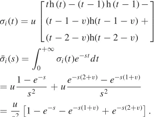
and constitutive equation: σ(t)=
t
−∞G (t−τ) ˙ε(τ) dτ (3) where σ,v, ε, ˙ε denote stress, mass velocity, strain and strain-rate.ρ and G(t) denote density of the material and the stress relaxation function. For generalized Maxwell viscoelastic solid, the stress relaxation function is
G (t)=Ee+ n
i=1 Eie−
t
θi. (4)
Where θi =ηi/Ei is the relaxation time of the each
Maxwell element, and the parameter Ee of the model
means that the solid materials cannot reduce the relaxation stress to zero.
As a simplified model, the stress relaxation function for a standard 3-element viscoelastic solid is
G (t)= E2 E1+E2
E1 +E2e−
t
θ
, θ= η E1+E2
· (5)
At time zero (t=0), the viscoelastic solid is static. The initial conditions are
σ(x,0)=0, ε(x,0)=0, v(x,0)=0, ˙ε(x,0)=0. (6) The boundary conditions will be depending on the different cases.
2.2. Solution of the image functions
For the time variable, we can transform the partial differential equation of the initial unknown function into ordinary differential equation of the image function by Laplace transforms method. The image function is denoted by the function with overline, whose transform variable is denoted by s. Combined with the initial conditions Eq. (6), the partial differential Eqs. (1)–(3) can be transformed to the follow equations:
¯ v= 1
ρs d ¯σ
d x (7)
¯˙
ε(s)= d ¯v
d x = 1 ρs
d2σ¯
d x2 (8)
¯ ε=1
s d ¯v d x =
1 ρs2
d2σ¯
d x2 (9)
¯
σ(s)=s ¯G(s)¯ε(s). (10) Where ¯G(s) denotes the stress function transformed by Laplace transform method. For the generalized Maxwell viscoelastic solid or the standard 3-element viscoelastic solid,
¯
G(s)= Ee
s +
n
i=1 Eiηi
Ei +ηis
· (11)
or,G(s)¯ = E2(E1 +ηs) s (E1+E2+ηs).
(12) The differential equation of the image function ¯σ(x,s) gives the result of the stress based on the Eqs. (7)–(10):
d2σ¯ d x2 =
ρs
G(s)σ.¯ (13)
In particular, for a standard 3-element viscoelastic solid, d2σ¯
d x2 =ρs
2E1+E2+ηs E2(E1+ηs) ¯
σ. (14)
The general solution of Eq. (13) is ¯
σ(x,s)=Ae(s)x+Be−(s)x (15) where(s)=√ρG(s)s is a root of the equation
2= ρs
G(s).For a standard 3-element viscoelastic solid, (s)=s√ρ
E2+(E1+ηs) E2(E1+ηs)
1 2
· (16)
Equation (15) gives the result of the stress for the image function ¯σ(x,s), where the coefficients A=A(s),B= B(s) would be solved with suitable boundary equations. More, we can confirm the image functions ¯v(x,s), ¯˙ε(x,s) and ¯ε(x,s) giving the results of the mass velocity, strainrate and strain. Then, the problems of the wave propagation would be solved numerically by way of numerical inverse Laplace transform.
3. 1D wave propagation in the
viscoelatic specimen occurred in SHPB
experiment
3.1. Derivation of the image function based on coupling boundary conditions
At time zero (t=0), the incident wave propagates to the left of the specimen along the right-bound characteristic line. According to the laws of the wave propagation along the right-bound characteristic line, we can confirm
σL(t)−σi(t)=ρ0c0[vL(t)−vi(t)]=
ρ0c0
vL(t)+ σρi(t)
0c0 .
Accordingly, the left boundary condition is
σL(t)=2σi(t)+ρ0c0vL(t). (17.1)
Whereρ0c0denotes wave impedance of the elastic bar. At the right of the specimen, the right boundary condition is σR(t)−0=−ρ0c0[vR(t)−0], which means
σR(t)=−ρ0c0vR(t). (17.2)
Combining with Eq. (7), Eq. (17) are transformed by Laplace transform to the follow image functions:
¯
σ(s,0)=2 ¯σi(s)+ ρρ0cs0σ¯x(s,0)
¯
σ(s,L)=−ρ0c0
ρs σ¯x(s,L)
· (18)
The general solution of image function for the stress Eq. (15) is substituted into the boundary condition Eq. (18). The coefficients A= A(s), B=B(s) would be solved:
A= 2 ¯σi(s) [1−1(s)] e −(s)L
[1−1(s)]2e−(s)L−[1+1(s)]2e(s)L B= −2 ¯σi(s) [1+1(s)] e
(s)L
[1−1(s)]2e−(s)L−[1+1(s)]2e(s)L· (19)
Where 1(s)= ρ0c0 ρs (s)=
ρ0√c0√s
ρ √G(s)1 . Especially, for
the standard 3-element elastic solid, the result is: (s)=s√ρ
E2 +(E1+ηs) E2(E1 +ηs)
1 2
1(s)= ρ√0c0 ρ
E2+(E1+ηs) E2(E1+ηs)
1 2 ·
Figure 1. A trapezoidal incident stress wave.
3.2. Exact solution to the problem of wave propagation in the elastic specimen
Due to space limitation, a special case when the specimen is pure elastic was solved analytically, giving the exact solution to the problem of elastic wave propagation in a sandwich elastic media. Here, the standard 3-element solid degrades into the pure elastic solid whose Young’s modulus is E2and elastic wave is
c=
E2
ρ.So, (s)=s
ρ
E2
= s
c, 1(s)= √ρ0c0
ρE2
= ρ0c0 ρc ·
The wave impedance ratio between the elastic bar and the specimen is denoted byλ=ρ0c0
ρc , and the elastic wave
propagation time in the specimen is denoted by T = Lc. Equation (20) is simplied:
A(s)= 2 1−λ
¯ σi(s)
1−µ2e2T s B(s)= −2
1−λ ¯
σi(s)µe2T s
1−µ2e2T s·
(21)
The image functions give the result of the stress of the two ends of the specimen:
¯
σLe f t= A(s)+B(s)=
2 ¯σi(s)
1−λ
1−µe2T s 1−µ2e2T s ¯
σRight =Ae(s)L +Be−(s)L =
−4λσ¯i(s)
(λ−1)2 eT s 1−µ2e2T s·
(22) In SHPB experiment, the incident wave is generally an approximate trapezoid. A incident wave is defined as Fig.1, and u, v denote the amplitude and width of the trapezoid wave. The rising and falling time is defined as 1 (non-dimensional value). The original function and image function of the incident wave are
σi(t)=u
t h (t)−(t−1) h (t−1)− (t−1−v)h(t−1−v)+ (t−2−v)h(t−2−v)
¯ σi(s)=
+∞
0
σi(t)e−stdt
=u1−e
−s
s2 +u
e−s(2+v)−e−s(1+v) s2
= u
s2
1−e−s−e−s(1+v) +e−s(2+v).
From the above equations, we can confirm the stress image functions of the two ends of the specimen. Using series expansion method, the problems was solved by way of inverse Laplace transform. The stress of the two ends of the elastic specimen is
σLe f t(t)=
2u 1−λ
∞
n=0
µ−2n−1(t−2nT )h(t−2nT )
−(t−2nT −1)h(t−2nT−1)
+(t−2nT −v−1)h(t−2nT −v−1)
+(t−2nT −v−2)h(t−2nT −v−2)
−µ−1(t−2nT −2T )h(t−2nT −2T )
−(t−2nT −2T −1)h(t−2nT −2T −1)
−(t−2n−2T −v−1)h(t−2nT−2T −v−1)
+(t−2nT −2T −v−2)h(t−2nT−2T −v−2) σRight(t)=(λ4u−1)λ2
∞
n=0 µ−2n−2
[(t−2nT −T )h(t−2nT −T )
−(t−2nT −T −1)h(t−2nT−T −1)
−(t−2nT −T −v−1)h(t−2nT −T −v−1)
+(t−2nT −T −v−2)h(t−2nT −T −v−2)]. (23) The analytical solution is compared with the numerical solution for the stress history at the left end of the specimen in Fig. 2a. Figure 2b shows the differences of the stress history between the two ends of the specimen.
If we define SHPB system as a wave propagation bar, the specimen between incident bar and transmission bar can be viewed as a impurity in the wave propagation bar which has imparity wave impedance. Figure 2b shows that the incident wave may change into the dispersive wave because of the transmission wave disturbed by the specimen when the incident wave pass through the elastic specimen. The phenomenon shows that the pure elastic may cause the dispersion.
3.3. Stress wave propagation in the viscoelastic specimen
0 2 4 6 8 10 0.000
0.005 0.010 0.015 0.020 0.025 0.030 0.035 0.040 0.045
FDM Analytical
Left side stress
Stress
Time
(a)
0 2 4 6 8 10
0.000 0.005 0.010 0.015 0.020 0.025 0.030 0.035 0.040 0.045
Left Right Incident
Time
(b)
Figure 2. (a) Stress profile on the left end of the specimen,
obtained by using series expansion method and finite difference simulation; (b) Stress profiles on both ends of the specimen.
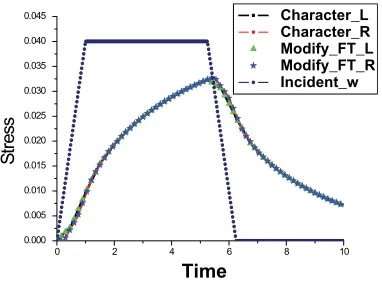
0 2 4 6 8 10
0.000 0.005 0.010 0.015 0.020 0.025 0.030 0.035 0.040
0.045 Character_L
Character_R Modify_FT_L Modify_FT_R Incident_w
St
re
ss
Time
Figure 3. Stress profile on both ends of the specimen, obtained
by using modified FT algorithm and finite difference simulation.
4. 1D stress wave propagation in the
semi-infinite viscoelatic bar
In the Laplace transform domain, the image functions at different positions in the bar are formulated by (15) and (16). Assuming that the viscoelastic bar is semi-infinited, we can ignore the effect of the right-end. It means
A=0. The boundary conditions of the left-end is σ(0,t )=σL(t), meaning B=σ¯(0,s)=σ¯L(s). The
im-age function of stress in the bar is
¯
σ(x,s)=σ0e −(s)x
s · (24)
Where (s)=√ρG(s)s , specially, for a standard 3-element viscoelastic solid,
(s)=s√ρ
E2+(E1+ηs) E2(E1+ηs)
1 2 .
In the case of strong discontinuity viscoelastic wave propagation in the Semi-Infinite bar, the image function of stress in the bar is
¯
σ(x,s)=σ0e −(s)x
s · (25)
For a standard 3-element viscoelastic solid, Eq. (25) is equivalent to
¯
σ(s)=σ0e−(s)x
s =
σ0 s exp
−T s
E2 +(E1+ηs) E1+ηs
= σ0
s e −T s
e
T s
1−
1+ E2
E1+ηs
(26) where, c=
E2
ρ, T =x/c denote the velocity of viscoelastic wave propagation and the time of the wave arriving at the location x. According to the lag theorem, the stress wave at the location x is
σ(x,t )=σ1(t−T ) h(t−T ). (27) The Laplace transform for theσ1(t) is
¯
σ1(s)= σ0
s exp
T s
1−
1+ E2 E1+ηs
· (28)
Assuming the time is infinite, we can get σ1(∞)=lim
s→0[s ¯σ1(s)]= σ0exp
lim
s→0T s
1−
1+ E2
E1+ηs =σ0.
(29)
At the time of the stress wave arriving the location x, the stress of the wavefront is
σ10+ = lim
s→∞[s ¯σ1(s)]=
σ0exp
!
lim
s→∞T s
1−
1+ E2
E1+ηs
"
· (30)
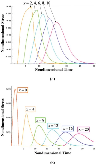
Figure 4. Stress histories at different sites of a viscoelastic bar
impacted at left end by (a) a trapezoidal stress pulse showed in Fig.1; (b) a half-sine stress pulse.
5. Summary
The viscoelastic wave propagation in the specimen of SHPB experiment was analyzed by Laplace transform
method. By conducting Laplace transform, the governing partial differential equations were transformed to ordinary differential equations for the image functions, which were solved analytically with the boundary equations of the two ends of the specimen. For viscoelastic specimen ,the problems was solved numerically by way of numerical inverse Laplace transform. For pure elastic specimen, it was solved analytically by Laplace transform.
The research was supported by National Science Foundation of China (11272163, 11390361). The part of the paper has been published in Chinese Journal of Theoretical and Applied Mechanics.
References
[1] Wang Lili. Stress Wave Foundation. Beijing: National Defense Industry Press, 2005 (in Chinese)
[2] Zhou Fenghua, Wang Lili, Hu Shisheng. On the effect of stress non-uniformness in polymer specimen of SHPB tests. Experimental Mechanics, 1992, 7(1):23– 29 (in Chinese)
[3] Wang L, Labibes K, Azari Z. Generalization of split Hopkinson bar technique to use viscoelastic bars. International Journal of Impact Engineering, 1994, 15: 669–686
[4] Zhao H, Gary G, Klepaczko JR. On the use of a viscoelastic splitHopkinson pressure bar. Inter-national Journal of Impact Engineering, 1997, 19: 319–330
[5] Subhash G, Liu Q, Gao XL. Quasistatic and high strain rate uniaxial compressive response of polymeric structural foams. International Journal of Impact Engineering, 2006, 32: 1113–1126