Design Wind Loads for Solar Modules Mounted Parallel to the Roof of a Low-rise Building

(1)

Scholarship@Western

Electronic Thesis and Dissertation Repository

4-17-2015 12:00 AM

Design Wind Loads for Solar Modules Mounted Parallel to the

Roof of a Low-rise Building

Sarah Elizabeth Stenabaugh

The University of Western Ontario

Supervisor Dr. G.A. Kopp

The University of Western Ontario

Graduate Program in Civil and Environmental Engineering

A thesis submitted in partial fulfillment of the requirements for the degree in Doctor of Philosophy

Follow this and additional works at: https://ir.lib.uwo.ca/etd

Part of the Civil Engineering Commons

Recommended Citation Recommended Citation

Stenabaugh, Sarah Elizabeth, "Design Wind Loads for Solar Modules Mounted Parallel to the Roof of a Low-rise Building" (2015). Electronic Thesis and Dissertation Repository. 2817.

https://ir.lib.uwo.ca/etd/2817

This Dissertation/Thesis is brought to you for free and open access by Scholarship@Western. It has been accepted for inclusion in Electronic Thesis and Dissertation Repository by an authorized administrator of

(2)

DESIGN WIND LOADS FOR SOLAR MODULES MOUNTED PARALLEL TO

THE ROOF OF A LOW-RISE BUILDING

(Thesis format: Monograph)

by

«Sarah Elizabeth Stenabaugh»

Graduate Program in Civil and Environmental Engineering

A thesis submitted in partial fulfillment of the requirements for the degree of

Doctor of Philosophy

The School of Graduate and Postdoctoral Studies The University of Western Ontario

London, Ontario, Canada

(3)

ii

Abstract

The focus of this study was to assess the wind induced pressures on an array of solar modules mounted parallel to the roof surface of a low-rise building. Wind tunnel studies were conducted on an array on a 1/20 scale building model with either a flat roof or a 30° roof slope. Specific attention was made to determine the effect of the spacing between individual modules, G, and the mounting height above the roof surface, H, resulting in a dataset of 80 configurations. Large G yielded improved wind resistance by lowering the external peak suctions and peak net suctions. Large H beyond a small cavity depth was determined to be detrimental for wind resistance as the peak external suctions were higher in magnitude and the cavity pressures more uniform (resulting in larger magnitude net suctions). Pressure equalization between the external and cavity pressures resulted in the net pressures being typically lower than the external pressures. The pressure

(4)

iii

Keywords

(5)

iv

Co-Authorship Statement

Dr. Gregory Kopp has been a very supportive and involved supervisor. He encouraged me through the process of defining the research problem and seeing through my plan. Under his guidance I designed and instrumented the wind tunnel model, supervised the tests and analyzed the data including the writing of all MATLAB code. The preparation of figures and text was done by me, aided by questions and input from Dr. Kopp. I received valuable design input from the University Machine Shop Services, who fabricated the model, and assistance from fellow students with testing the numerous configurations.

Selected elements from the work presented herein have been published in the Journal of Wind Engineering and Industrial Aerodynamics. The article, “Wind loads on

photovoltaic arrays mounted parallel to sloped roofs on low-rise buildings”, was

published online on the 30th_{of January, 2015. It presents a validation of the sloped roof} model, pressure coefficients, and pressure equalization coefficients (elements of chapters 3 & 5). This article was coauthored by Yumi Iida, Dr. Gregory Kopp and Dr. Panagiota Karava. Yumi Iida was an exchange student at the Boundary Layer Wind Tunnel Laboratory in 2007 and 2008. She assisted with conducting the wind tunnel studies and was instrumental in making the sheer number of configurations manageable. Dr. Kopp as my supervisor aided with the overall direction, theme and message of the paper through many discussions. Dr. Karava was my undergraduate thesis supervisor and started me on this subject. Her guidance in the initial stages is very much appreciated.

(6)

v

Acknowledgments

My experience at the Boundary Layer Wind Tunnel Laboratory at the University of Western Ontario has been a positive one, largely due to the assistance and encouragement I received from a number of individuals associated with the lab and facilities.

Thank you to my supervisor, Dr. Greg Kopp, for providing me with opportunities to gain knowledge and experience. Thank you to the wind tunnel technicians, Mr. Gerry Dafoe and Mr. Anthony Burggraaf, for their assistance and patience. The staff at University Machine Shop Services fabricated my experimental model and their attention to detail and design capabilities were instrumental to my research. Mrs. Karen Norman is nothing short of amazing and has been a continuous source of support and guidance. Thank you to my fellow students, most notably Dr. Adam Kirchhefer and Dr. Maryam Refan, for their advice and perspective, for lending a helping hand and for their friendship. I look forward to maintaining these connections throughout our careers, wherever they take us.

(7)

vi

List of Tables

Table 1: Gap, height and array dimensions ... 31

Table 2: G/H and Phi values calculated using the equation and definition for the single cavity for multiple H data adapted from Oh and Kopp 2015 ... 76

Table 3:Phi values a small cavity depth from Oh and Kopp 2015 G = 1 mm; H = 1.2 mm and the current study G = 12 cm; H = 2 cm on the flat roof ... 81

Table 4:Phi values for a large cavity system from Oh and Kopp 2015 G = 1 mm; H = 15 mm and the current study G = 12 cm; H = 20 cm on the flat roof ... 83

Table 5: Roof edge zone widths from design standards and literature for flat roof model ... 123

Table 6: Analysis cases representing combinations of array and roof zones considered for the development of the roof zone factor, γR, and the array zone factor, γE ... 132

Table A1: Sloped-roof configurations (base configurations, original 42) ... 158

Table A2 : Flat-roof configurations ... 159

Table A3 : Shroud sloped-roof configurations ... 159

Table A4: Shroud flat-roof configurations ... 160

(11)

x

List of Figures

Figure 1-1: Sketch of the conical vortices from a cornering wind direction with secondary separation and reattachment lines (adapted from Holmes, 2007 and Bienkiewicz and Sun, 1992) ... 7

Figure 1-2: Roof zones and external pressure coefficients for 27 – 45° gable roof slopes adapted from ASCE 7-10 (2010) ... 15

Figure 1-3: Roof zones and nominal net pressure coefficients adapted from SEAOC PV2-2012 (PV2-2012) ... 19

Figure 1-4: Sketch of edge and sheltered modules with array edge factors adapted from SEAOC PV2-2012 (2012) ... 20

Figure 2-1: Photo of sloped roof model ... 27

Figure 2-2: Mean wind speed and streamwise turbulence intensity profiles ... 28

Figure 2-3: Longitudinal spectrum measurements from the wind tunnel for z0 = 0.01 m 29

Figure 2-4: Drawings of the array denoting the gap, G, and height, H, variables ... 31

Figure 2-5 Scale model of a) the flat-roof model and b) the sloped model with the shroud surrounding the array ... 32

Figure 2-6 Photos of the array taped in the 2x2 set-up (left) and 4x4/3x4 (right) ... 33

Figure 2-7: Simulated larger module dimensions ... 34

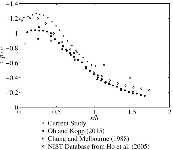
Figure 3-1: Mean point pressure coefficients from the sloped roof model - comparison with previous studies ... 41

(12)

xi

Figure 3-3: Contour map of instantaneous external point pressures resulting in peak external suction G≈ 0; H≈ 0 (left) and mean external point pressures for the peak wind direction of 112.5° (right) ... 44

Figure 3-4: Contour map of instantaneous external point pressures resulting in peak external suction G≈ 0; H = 20 cm (left) and mean external point pressures for the peak wind direction of 292.5° (right) ... 45

Figure 3-5: Contour map of instantaneous external point pressures resulting in peak external suction G = 12 cm; H≈ 0 (left) and mean external point pressuresfor the peak wind direction of 315° (right) ... 46

Figure 3-6: Contour map of instantaneous cavity point pressures at the instant of peak external suction for the G = 12 cm; H≈ 0 configuration (left) and mean cavity point pressuresfor the peak (external) wind direction of 315° (right) ... 46

Figure 3-7: Contour map of instantaneous cavity point pressures resulting in peak cavity suction G≈ 0; H≈ 0 (left) and mean cavity point pressuresfor the peak wind direction of 67.5° (right) ... 48

Figure 3-8: Contour map of instantaneous cavity point pressures resulting in peak cavity suction G≈ 0; H = 20 cm (left) and mean cavity point pressures for the peak wind

direction of 90° (right) ... 49

Figure 3-9: Contour map of instantaneous cavity point pressures resulting in peak cavity suction G = 12 cm; H = 20 cm (left) and mean cavity point pressures for the peak wind direction of 90° (right) ... 50

(13)

xii

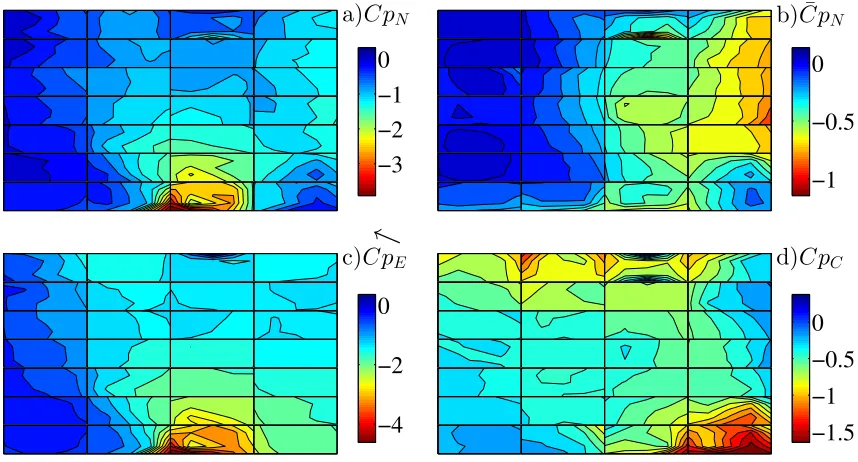
Figure 3-11: Contour map of a) instantaneous net point pressures resulting in peak net suction G≈ 0; H≈ 0, b) mean net point pressures for the peak wind direction of 112.5°, c) instantaneous external and d) cavity point pressures that resulted in peak net suction 53

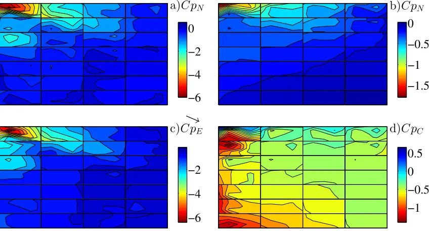
Figure 3-12: Contour map of a) instantaneous net point pressures resulting in peak net suction G≈ 0; H = 20 cm, b) mean net point pressures for the peak wind direction of 292.5°, c) instantaneous external and d) cavity point pressures that resulted in peak net suction ... 54

Figure 3-13: Contour map of a) instantaneous net point pressures resulting in peak net suction G = 12 cm; H≈ 0, b) mean net point pressures for the peak wind direction of 315°, c) instantaneous external and d) cavity point pressures that resulted in peak net suction ... 55

Figure 3-14: Distribution of the external-cavity point pressure correlation coefficients for the peak wind direction of 112.5° (G≈ 0; H≈ 0) ... 56

Figure 3-15: Distribution of the external-cavity point pressure correlation coefficients for the peak wind direction of 292.5° (G≈ 0; H = 20 cm) ... 57

Figure 3-16: Distribution of the external-cavity point pressure correlation coefficients for the peak wind direction of 315° (G = 12 cm; H≈ 0) ... 58

Figure 3-17: The worst case values of the peak (suction) external area-averaged over a single module on (a) the external, upper, surface, (b) in the cavity, and (c) net with respect to H ... 60

Figure 3-18:The worst case values of the peak (suction) external area-averaged over a single module on (a) the external, upper, surface, (b) in the cavity, with respect to G .... 60

Figure 3-19: Contour map of instantaneous external point pressure coefficients resulting in peak external uplift G = 12 cm; H≈ 0 (left) and mean external point pressure

(14)

xiii

Figure 3-20: Contour map of instantaneous cavity point pressure coefficients resulting in peak cavity suction G = 12 cm; H≈ 0 (left) and mean cavity point pressure coefficients for the peak wind direction of 45° on the flat roof (right) ... 64

Figure 3-21: Contour map of instantaneous cavity point pressure coefficients resulting in peak cavity suction G = 12 cm; H = 20 cm (left) and mean cavity point pressure

coefficientsfor the peak wind direction of 180° on the flat roof (right) ... 64

Figure 3-22: Distribution of the external-cavity point pressure correlation coefficients for the peak wind direction of 45° on the flat roof (G = 12 cm; H≈ 0) ... 65

Figure 3-23 Contour map of a) instantaneous net point pressures resulting in peak net uplift for the G = 12 cm; H≈ 0 flat roof configuration, b) mean net point pressure coefficient for the same (peak) wind direction of 45°, c) instantaneous external and d) instantaneous cavity point pressures that resulted in peak net uplift ... 66

Figure 3-24: Contour map of a) instantaneous net pressure resulting in peak net point pressure for the G = 12 cm; H = 20 cm flat roof configuration, b) mean net point pressure coefficient for the same (peak) wind direction of 45°, c) instantaneous external and d) instantaneous cavity point pressures that resulted in peak net uplift ... 67

Figure 3-25: The worst case values of the peak (suction) external area-averaged over a single module on (a) the external, upper, surface, (b) in the cavity, and (c) net with respect to H for the sloped roof model (grey) and the flat roof model (black) ... 68

Figure 4-1: Sample external (black) and cavity (grey) pressure time histories, area-averaged over a single module for a) a sampling period of 10 seconds and b) ½ second before and after the largest measured external suction ... 71

(15)

xiv

Figure 4-3: External and cavity RMS values for module 1 (upper) and module 14 (lower) with respect to wind direction for G = 12 cm; H = 20 cm and G = 12 cm; H = 2 cm on the sloped roof ... 73

Figure 4-4: Sketch of external and cavity pressure distributions for φ < 1 and φ > 1 ... 75

Figure 4-5: External and cavity pressures along a line of taps for a single cavity for multiple H (adapted from Oh and Kopp 2015) ... 76

Figure 4-6: Mean external and cavity pressures along multiple modules; G = 1 mm; various H from Oh and Kopp (2015) ... 78

Figure 4-7: Comparison of mean external and cavity pressures along a single tap line from G = 1 mm; H = 1.2 mm (Oh and Kopp, 2015) and G = 12 cm; H = 2 cm flat roof configuration (270°) from the current study with respect to x/h ... 79

Figure 4-8: Comparison of mean external and cavity pressures along a single tap line from G = 1 mm; H = 1.2 mm (Oh and Kopp, 2015) and G = 12 cm; H = 2 cm flat roof configuration (270°) from the current study normalized over module length ... 81

Figure 4-9: External and cavity pressures along a line of taps for a multiple modules for G = 15 mm; H = 1.2 mm (adapted from Oh and Kopp 2015) ... 82

Figure 4-10: Comparison of mean external and cavity pressures along a single tap line from G = 1 mm; H = 15 mm (Oh and Kopp, 2015) and G = 12 cm; H = 20 cm flat roof configuration (270°) from the current study normalized over module length ... 83

Figure 5-1: Pressure equalization coefficient for single modules with respect to H ... 87

Figure 5-2: Pressure equalization coefficient for single modules with respect to G ... 88

(16)

xv

Figure 5-4: Pressure equalization coefficients with respect to the G/H ratio for four tributary areas from the sloped roof (open markers) and flat roof (solid markers) models ... 91

Figure 5-5: Pressure equalization coefficients with respect to the G/H ratio simulating three module sizes from the sloped roof (left) and flat roof (solid right) models ... 93

Figure 5-6: Worst, peak, cavity (suction) coefficients area-averaged over three areas simulating different module sizes plotted with respect to the G/H ratio from the sloped roof (left) and flat roof (solid right) models ... 94

Figure 5-7: Worst, peak, external (suction) coefficients area-averaged over three areas simulating different module sizes plotted with respect to the G/H ratio from the sloped roof (left) and flat roof (solid right) models ... 94

Figure 5-8: Worst, peak, net (suction) coefficients area-averaged over three areas simulating different module sizes plotted with respect to the G/H ratio from the sloped roof (left) and flat roof (solid right) models ... 95

Figure 5-9: Pressure equalization coefficients with respect to the G/H ratio simulating three module sizes from the sloped roof (left) and flat roof (solid right) models with values from the sealed data plotted with respect to effective (lower) G/H superimposed in red ... 96

Figure 5-10: Peak net suctions (left) and pressure equalization coefficients (right) with respect to G/H for two different aspect ratios ... 97

Figure 5-11: Peak net suctions (left) and pressure equalization coefficients (right) with respect to G/H for three different aspect ratios ... 98

Figure 6-1: Plan view of the flat roof model ... 100

(17)

xvi

Figure 6-3: Conceptual flow patterns on the external (upper) surface of the array and in the cavity for a range of H (inspired by from Malavasi and Trabucchi, 2008; Blois and Malavasi, 2007; Martinuzzi et al., 2003; and Auteri et al., 2008) ... 104

Figure 6-4: External peak suctions, mean and RMS pressure coefficients measured along the top row of pressure taps on the middle row of modules for the 270° wind direction for the G = 12 cm configurations on the flat roof ... 107

Figure 6-5: External mean and RMS pressure coefficients measured along the top row of pressure taps on the middle row of modules for the 270° wind direction for the G = 12 cm configurations on the flat roof ... 108

Figure 6-6: Cavity mean and RMS pressure coefficients measured along the top row of pressure taps on the middle row of modules for the 270° wind direction for the G = 12 cm configurations on the flat roof ... 109

Figure 6-7: External mean and RMS pressure coefficients measured along the bottom row of pressure taps on the bottom (field) row of modules for the 225° wind direction for the G = 12 cm configurations on the flat roof ... 110

Figure 6-8: External mean and RMS pressure coefficients measured along two tap lines on the column of modules adjacent to the field of the roof for the 225° wind direction for the G = 12 cm configurations on the flat roof ... 111

Figure 6-9: External mean and RMS pressure coefficients measured along two tap lines on an interior column of modules for the 180° wind direction for the G = 12 cm

configurations on the flat roof ... 112

(18)

xvii

Figure 6-11: External mean and RMS pressure coefficients measured along the top row of pressure taps on the middle row of modules for the 270° wind direction for the G ≈ 0 configurations on the sloped roof ... 115

Figure 6-12: Cavity mean and RMS pressure coefficients measured along the top row of pressure taps on the middle row of modules for the 270° wind direction for the G ≈ 0 configurations on the sloped roof ... 115

Figure 6-13: Array edge zone as approximated by ≈ 1(H + t) to 2(H + t) (left) and as used for developing design recommendations (right) ... 116

Figure 6-14: The worst case values of the peak (suction) (a) external, (b) cavity, and (c) net pressure coefficients, area-averaged over a single solar module and (d) the pressure equalization coefficient (Ceq) with respect to H; considering only the interior modules. ... 118

Figure 6-15: The worst case values of the peak (suction) (a) external, (b) cavity, and (c) net pressure coefficients, area-averaged over a single solar module and (d) the pressure equalization coefficient (Ceq) with respect to G; considering only the interior modules. ... 119

Figure 6-16: The peak maxima pressure equalization coefficient (Ceq) for the edge and interior zones for the single module area (0.73m2) with respect to G/H for the sloped and flat roof models ... 120

Figure 6-17: Peak net (suction) pressure coefficients with respect to H measured in each roof zone on the flat roof model (G = 12 cm) ... 122

Figure 6-18: The peak net (suction) coefficient measured on each module for the G = 12 cm; H = 20 cm (left) and G = 12 cm; H≈ 0 (right) configurations on the flat roof model ... 123

(19)

xviii

Figure 6-20: The pressure equalization coefficient (left) and the mean net pressure coefficient (right) for open and shrouded array for G = 12; H = 20 cm and G = 12; H = 2 cm on the flat roof model ... 126

Figure 6-21: The mean external (left) and the mean cavity (right) pressure coefficient for open and shrouded array for G = 12; H = 20 cm and G = 12; H = 2 cm on the flat roof 127

Figure 6-22: Mean external point pressure contours for the a) G = 12 cm; H = 20 cm open array, b) G = 12 cm; H = 2 cm open array, c) G = 12 cm; H = 20 cm shrouded array and d) G = 12 cm; H = 2 cm shrouded array on the flat roof model ... 128

Figure 6-23: Mean cavity point pressure contours for the a) G = 12 cm; H = 20 cm open array, b) G = 12 cm; H = 2 cm open array, c) G = 12 cm; H = 20 cm shrouded array and d) G = 12 cm; H = 2 cm shrouded array on the flat roof model ... 129

Figure 6-24: Schematic of potential aerodynamic shroud to mitigate array edge effects ... 130

Figure 7-1: Schematic of modules used to evaluate the pressure equalization coefficient for the different array and roof zone cases considered for design for the flat roof model ... 134

Figure 7-2: Schematic of modules used to evaluate the pressure equalization coefficient for the different array and roof zone cases considered for design for the sloped roof model... 135

Figure 7-3: Pressure equalization coefficients with respect to tributary area and design factor γR for a); roof zone 1 and G/H < 1, b) roof zone 1 and G/H≥ 1, c) roof zone 2 and G/H < 1, d) roof zone 2 and G/H≥ 1 ... 137

(20)

xix

Figure 7-5: Pressure equalization coefficients with respect to tributary area and design factors γR and γR·γE where γE is a separate value for a) roof zone 1 and G/H < 1, b) roof

zone 1 and G/H≥ 1, c) roof zone 2 and G/H < 1, d) roof zone 2 and G/H≥ 1 ... 139

Figure 7-6: Possible design figure to evaluate γR and table to determine γE ... 140

Figure 7-7: Pressure equalization coefficients with respect to tributary area and design factors γR and γR·γE for a) roof zone 1 and G/H < 1, b) roof zone 1 and G/H≥ 1, c) roof zone 2 and G/H < 1, d) roof zone 2 and G/H≥ 1 ... 141

Figure 7-8: Design factor, γ, for solar installations mounted parallel to roof surfaces of low-rise buildings to be applied to the external pressure coefficient from the components and cladding procedure in existing design standards ... 142

Figure A1 : Model dimensions - sloped roof model ... 156

Figure A2 : Model dimensions - flat roof model ... 157

Figure A3 : Tap labels for pressure taps on the upper surface of the array ... 161

Figure A4 : Tap labels for pressure taps on the lower surface of the array ... 161

Figure A5: Tap labels for pressure taps on the roof surface (G=0 roof piece shown) .... 162

Figure A6 : Tap locations on the individual modules ... 162

Figure B1: Instantaneous external pressure coefficients resulting in the peak external suction, area-averaged over a single module for the G≈ 0; H≈ 0 configuration on the sloped roof model ... 164

(21)

xx

Figure B3: Instantaneous external pressure distribution, evaluated for the individual modules, which results in the peak external suction, area-averaged over a single module for the G≈ 0; H≈ 0 configuration on the sloped roof model ... 166

Figure B4: Instantaneous external pressure coefficients resulting in the peak external suction, area-averaged over a single module for the G≈ 0; H = 20 cm configuration on the sloped roof model ... 166

Figure B5: Instantaneous external pressure distribution, evaluated for the entire array, which results in the peak external suction, area-averaged over a single module for the G≈ 0; H = 20 cm configuration on the sloped roof model ... 167

Figure B6: Instantaneous external pressure distribution, evaluated for the individual modules, which results in the peak external suction, area-averaged over a single module for the G≈ 0; H = 20 cm configuration on the sloped roof model ... 168

Figure B7: Instantaneous cavity pressure coefficients resulting in the peak cavity suction, area-averaged over a single module for the G≈ 0; H = 20 cm configuration on the sloped roof model ... 168

Figure B8: Instantaneous cavity pressure distribution, evaluated for the entire array, which results in the peak cavity suction, area-averaged over a single module for the G≈ 0; H = 20 cm configuration on the sloped roof model ... 169

Figure B9: Instantaneous cavity pressure distribution, evaluated for the individual

modules, which results in the peak cavity suction, area-averaged over a single module for the G≈ 0; H = 20 cm configuration on the sloped roof model ... 170

(22)

xxi

Figure B11: Instantaneous external pressure distribution, evaluated for the entire array, which results in the peak external suction, area-averaged over a single module for the G = 12 cm; H≈ 0 configuration on the sloped roof model ... 171

(23)

xxii

List of Appendices

Appendix A: Wind tunnel testing details ... 156 Appendix B: Different contouring approaches for peak pressure coefficient

distributions ... 164

(24)

xxiii

List of Nomenclature

The nomenclature used throughout the thesis is listed below. The source for design code parameters is indicated in parenthesis where applicable.

A tributary area

a parameter to set the dimensions of roof zones (ASCE 7-10) ai weighted area for area-averaged pressure

apv parameter to set the dimensions of roof zones (SEAOC PV2-2012)

B length of the model

c combination of modules Ceq pressure equalization coefficient CL orifice loss coefficient

instantaneous external (upper surface) pressure coefficient

̅ _{mean external (upper surface) pressure coefficient}

area-averaged external (upper surface) pressure coefficient

̅ _{area-averaged, mean external pressure coefficient}

area-averaged, Lieblein-fitted, peak (suction) external pressure coefficient instantaneous cavity (upper surface) pressure coefficient

area-averaged cavity pressure coefficient

̅ _{area-averaged, mean cavity pressure coefficient}

area-averaged, Lieblein-fitted, peak (suction) cavity pressure coefficient instantaneous net (upper surface) pressure coefficient

area-averaged net pressure coefficient

̅ _{area-averaged, mean net pressure coefficient}

area-averaged, Lieblein-fitted, peak (suction) net pressure coefficient dx module set-back from roof edge (SEAOC PV2-2012)

E array edge factor (SEAOC PV2-2012)

f frequency

fH cavity friction coefficient

ft orifice friction coefficient

(25)

xxiv

G/H system relative permeability

(GCp) external pressure coefficient (ASCE 7-10) (GCpi) internal pressure coefficient (ASCE 7-10)

(GCrn) combined net pressure coefficient (SEAOC PV2-2012)

(GCrn)nom nominal net pressure coefficient (SEAOC PV2-2012)

H cavity depth

h mean roof height for sloped-roof model; eave height for flat roof model hc characteristic height (SEAOC PV2-2012)

h1 height between roof surface and lower end of module (SEAOC PV2-2012)

kz exposure factor (ASCE 7-10)

kzt topography factor (ASCE 7-10)

kd directionality factor (ASCE 7-10)

L module length

Lc effective cavity length

n point pressures considered for area-averaged pressures p design wind pressure (ASCE 7-10)

qh velocity pressure (ASCE 7-10)

Re Reynolds number

ReH Reynolds number in the cavity

t module thickness

mean streamwise velocity in the wind tunnel mean streamwise velocity in the cavity

mean streamwise velocity at mean or eave roof height V basic wind speed (ASCE 7-10)

WL width of building on longer building side (SEAOC PV2-2012)

z0 roughness length

γ proposed design multiplication factor γC chord factor (SEAOC PV2-2012) γE array zone factor

(26)

xxv

∆ ̅ mean pressure drop through the cavity

∆ ̅ mean pressure drop through the orifice θ wind direction

length scale velocity scale

kinematic viscosity of air

φ parameter to predict of cavity pressure distribution ω module tilt angle (SEAOC PV2-2012)

(27)

1

Introduction

Awareness of our energy consumption as a society is increasing, as is the desire to locally produce energy using so-called “green technologies”. One possible source of green energy is roof-mounted solar, photovoltaic (PV), modules. These modules (sometimes referred to as panels) cover roof surfaces and, thus, are exposed to the elements,

including wind. To ensure that the system is adequately designed to withstand the forces expected to act on it during its lifetime, the wind loading on these modules needs to be determined. The majority of building-mounted solar arrays are placed on the roofs of low-rise buildings, so it is the wind field above such structures which control the wind loads. The flow environment and aerodynamics of low-rise buildings are complex due to the interactions of the turbulence in the wind with the turbulence and vortices generated by the large-scale flow separations from the buildings themselves. This leads to large uplift forces on low-rise building roofs, but is also a challenging flow environment for roof-mounted equipment such as solar arrays. Boundary layer wind tunnels can be used to test scale models of roof-mounted solar systems in a multitude of configurations to determine the effect of multiple design variables in an economical and timely fashion and ultimately develop design standards.

1.1 Background and Motivation

(28)

1.2 Previous testing of tilted solar arrays mounted on

flat roofs

Over the past decade, roof-mounted solar systems have tended to be tilted arrays of multiple modules installed on the large, low-slope, commercial roofs of low-rise

structures. The lack of design provisions in building codes for these initial installations, coupled with their magnitude in size and cost of installation, justified wind tunnel studies to examine the aerodynamics, as well as to quantify the loads. Some of the notable studies include Geurts and van Bentum 2006, 2007; Kopp et al., 2012; Banks, 2013; Kopp 2013; Kopp and Banks; 2013, Cao et al.; 2013; Maffei et al., 2013; and Pratt and Kopp, 2013; although early studies were conducted by Tieleman et al., (1980). These studies identified the role of the building geometry (i.e., building height, plan dimensions, parapet height) and array geometry (panel tilt angle, chord, tributary area, gaps between rows, clearance of panel above roof surface, distance from edge of roof, etc.) in setting the wind loads.

Kopp (2013) noted that the determination of aerodynamic forces, uplift in particular, is crucial for the design of tilted arrays installed on the flat roof of low-rise buildings as they govern the required ballast, or roof penetration, to resist uplift. The forces can be complicated since the wind field is influenced not only by the natural turbulence of wind but also from vortices and separation along building edges (Kopp et al., 2012). It has been established that building size, which controls the size of vortices on the roof, plays an important role in setting the wind loads on low-profile, tilted, roof-mounted arrays (Kopp et al., 2012; Banks, 2013; Pratt and Kopp, 2013). This is due to the conical vortices from cornering wind directions which are strengthened by vortex stretching and continuous separation along the building walls; as such larger wind loads are measured on larger buildings (Kopp et al., 2012, Banks, 2013). The strength of the vortex is

(29)

tilt and swirl direction of the corner vortex. The corner vortices have also been noted to increase the wind loads on the array when there is a parapet (Browne et al., 2013; Banks, 2013).

While the building on which the array is mounted plays a significant role in determining the array wind loads, so too does array geometry. Kopp et al. (2012) found that larger modules were associated with an increase in the wind loads for the higher tilt models, but that module dimensions had minimal impact on the lower tilt systems. The same study reported that the loading mechanisms were different depending on the tilt angle of the modules. They reported that wind pressures on low-tilt arrays (5°) were governed by pressure equalization across the modules from the building generated (roof) pressures, while higher tilt arrays (30°) were influenced by generated flow. The array-generated flow served to augment the loads caused by pressure equalization with the 2° tilt angles having loads approximately 30 – 40% smaller than for 10° tilt (and larger) angles (Kopp, 2013). The same study also found that neither the row spacing nor the minimum height above the roof surface (when kept below 0.41m) had an impact on the net wind loads.

(30)

With the pressures on the array sensitive to the building induced vortices, it can be

deduced that the aerodynamics of roof mounted systems differ from those that are ground mounted. This is due to the fact that they would not be subjected to the

building-generated flow field. This was confirmed with simultaneous pressure measurements and particle image velocimetry (PIV) to measure the flow field in an experiment performed by Pratt and Kopp (2012). They noted that it was the vertical velocity component in the vortex, caused by the separated flow off the building edge, which caused the largest uplift on the solar panels.

Wind loads from some of these studies are beginning to appear in design standards such as NEN 7250 (2013) and SEAOC PV2-2012 (2012). However, another fairly common type of roof-mounted array, those with modules parallel to the surface of pitched roofs, usually houses, has received less attention even though such systems are relatively common in some jurisdictions. Design standards specific to solar modules mounted parallel to roof slopes are still underdeveloped with additional wind tunnel studies required to solidify our understanding of the wind loading mechanisms.

1.3 Previous testing of solar modules mounted parallel

to roofs

(31)

(due to positive pressures acting on the underside of the panel near the ridge), consistent with the findings of Aly and Bitsuamlak (2014) who also studied scale models of solar modules mounted parallel to a sloped gable roof surface.

Geurts and Blackmore (2013) conducted full-scale and model-scale tests of a single solar module mounted on a hip roof. Since this study was of a single module there were no modeled gaps, just as for the studies of Stenabaugh et al. (2010, 2011) and Ginger et al. (2011), although the module was of a considerably smaller size. Geurts and Blackmore found that while the effect is small, external peak pressures on the upper surface are higher for larger H. On the underside of the module, peak positive cavity pressures were found to be larger with larger H, while peak suctions were found to be smaller in

magnitude over the range they examined. They found strong correlations between the external and cavity pressures which resulted in relatively small net wind loading due to pressure equalization. Levels of pressure equalization were significantly different from those found in the studies of Stenabaugh et al. (2010, 2011) and Ginger et al. (2011), whose modules were much larger in size. Thus, the generality of the conclusions is not clear for arrays made up of many modules, where gaps between individual modules could alter the local flow-field and influence cavity and net wind pressures, as they do for roof pavers (e.g., Bienkiewicz and Sun, 1992, 1997; Asghari Mooneghi et al., 2014) and other roof-mounted systems (Oh and Kopp, 2014). The omission of modeled gaps could possibly yield substantially different aerodynamics and net wind loads on the panels than what exists in reality.

1.4 Loose-laid paving systems

The most relevant work on both the effects of gaps between modules and the cavity depth has been done on loose-laid paver systems installed on flat-roofed, low-rise, buildings (Kind and Wardlaw, 1982; Bienkiewicz and Sun, 1992, 1997; Asghari Mooneghi et al., 2014). Loose-laid pavers are part of double-layer roofing systems, which are sometimes used on flat-roofed, low-rise, commercial structures. Kind and Wardlaw (1982)

(32)

opposed to tight fitting joints). Bienkiewicz and Sun (1992, 1997) studied scaled paver installations on the flat roof of a low-rise building in a wind tunnel for a cornering wind direction. Of particular interest to them were the cavity pressures. They found that a cavity beneath the modules, even a small one (i.e., ¼ paver thickness, t), significantly reduced the peak and mean cavity pressures. The cavity pressure distributions with relatively larger cavity depths (i.e., ½ t) were found to be more uniform due to reduced flow resistance. Larger cavity depths (i.e., ≥ ¼ t) were not found to have a large impact on either the cavity pressure distributions or the peak suctions once they are over a particular size. In particular, a cavity that was a ¼ of the paver’s thickness yielded a significant reduction in the peak cavity suction with no increased reduction for cavities up to the paver thickness.

Conical vortices are produced from a cornering wind, causing lines on the roof where the flow reattaches (R) and separates (S) for a second time due to the rotation of the vortex (i.e., Bienkiewicz and Sun, 1992 and Holmes, 2007). A schematic of these vortices has been adapted from existing literature and is shown in Figure 1-1. Bienkiewicz and Sun found that the correlation coefficients between the external (upper surface) and cavity pressures were close to unity (with the exception of three pavers near the roof corner) when the pavers were installed without a cavity (H≈ 0) and influenced by the

(33)

F se B A tu m sp n w w w p ob eq in sy re up at ra b an

Figure 1-1: S econdary se Bienkiewicz

A related stu unnel studies model and set pecifically e

oted that wh was in the Bie were installed wind uplift ca ermeability bserved that qualization i ncreasing an ystem with t educed to ⅔

plift was fou t the Wall of atios leading e noted the s nd Asghari M

Sketch of th eparation an

and Sun, 19

udy published s of loose-lai

t-up as the p xpanded the hile there wa enkiewicz an d with some an be reduce (G) and the t with larger increased, as d approachin tightly packe

of the extern und to be onl f Wind, whic g to reduced

studies by B Mooneghi et

he conical vo nd reattachm 992)

d by Bienkie id paver syst previous pav e scope to inc as no mention nd Sun studi

gap, rather t ed with large flow resistan

values of th s indicated b ng the limit ed modules ( nal pressure ly ½ the exte ch confirmed net loads (A ienkiewicz a t al., 2014 on

ortices from ment lines (

ewicz and En tems on flat er studies by clude the eff n of what th ies (1992, 19 than sealed. er G and that

nce in the ca he system rel by the magni of the extern (small G) an

. If the cavit ernal pressur d the depend Asghari Moon

and Sun (199 nly consider

m a cornerin (adapted fro

ndo (2009) a roofs. They y Bienkiewic fect of gaps b

e experimen 997), it can b

Bienkiewic t the reductio avity (contro lative perme itude of the t nal (upper su nd some cavi

ty depth was re. Large-sc dence on the

neghi et al., 92, 1997), B red a single,

ng wind dire om Holmes,

also focused y used the sa cz and Sun ( between pav ntal gap, G, b be inferred th cz and Endo

on depends o olled by H).

ability, G/H transmitted ( urface) press ity depth, the

s further red cale studies w e G/H ratio, w 2014). How Bienkiewicz

cornering, w

ection with , 2007 and

d on the wind ame wind tun (1992, 1997) vers. It shou between pav hat the pave (2009) note on the

They furthe H, pressure

(cavity) pres sure. For a e net uplift w duced, the ne

were perform with higher wever, it sho

(34)

While it is known that a cornering wind is typically associated with the peak suction wind loads on the roof, it is possible that the presented pressure coefficients may not have captured the worst cases needed for design.

(35)

cavity. It is clear that the gap between modules and cavity depth for roof-mounted solar arrays are significant parameters that need to be considered in the design wind loads for arrays mounted parallel to the roof surface. Together they influence the degree of pressure equalization, which has been noted for its significance in setting the wind loads for both (low) tilted solar arrays and loose-laid pavers on flat roofs of low-rise structures.

1.5 Pressure

equalization

Roof mounted solar arrays can be considered a double layer system – with the roof as the inner layer and the modules as the outer layer just as roof pavers are. The external (upper) surface and cavity (lower surface of the modules) are exposed to wind flow since there is a void beneath the roof and the underside of the modules. Pressure equalization is a wind loading process that can occur; with the cavity pressure partially approaching that on the upper (external) surface of the array. Perfect pressure equalization is unlikely in practice (since it could only happen for static, uniform, external pressures), however, net pressures on roof-mounted pavers have been found to be less that what would be expected on the bare roof due to this process (Bienkiewicz and Endo, 2009). As such, pressure equalization can play a crucial role in reducing the (net) design wind loads for the outer layer of double layer systems (see Bienkiewicz and Endo, 2009 for roof pavers and Kopp, 2014 for tilted solar installations on flat roofs). The process of pressure equalization is not limited to roof pavers and solar modules, but also impacts cladding systems such as curtain walls, brick veneer or vinyl siding walls, and rainscreen walls (Kumar, 2000).

(36)

addition to the dimensions of both the cavity and the vented openings, are key design parameters. Small, deep vents lead to laminar flow, with turbulent flow associated with vents that are large in cross-section, yet shallow in depth (Cook, 1990). Smaller cavities require less airflow to achieve equalization and thus yield a faster response time – important when designing for the short duration peaks across the rainscreen (Kumar, 2000).

While vents are beneficial in ensuring pressure equalization for rainscreens, a similar statement can be made regarding gaps for loose-laid pavers. As previously mentioned, Kind and Wardlaw (1982) found that the inclusion of gaps between individual paver elements could actually prevent the failure when performing blow-off tests. This indicates that resistance to failure of individual pavers was increased when the pavers were not flush with one another but separated by an air gap. In 1991, Okada and Okabe tested failure wind speeds of paver systems with two different cavity depths. They found that a cavity depth (not loose-laid, but mounted with an offset from the roof) resulted in lower failure wind speeds due to relatively poorer pressure equalization. Thus, while gaps are beneficial, relatively large cavity depths are detrimental to pressure equalization, consistent with the discussion on pavers in section 1.4 where pressure equalization is noted to be improved with higher values of G/H.

While large cavity depths may not be optimal with respect to increasing pressure equalization, they are a required component of dual-layer wall or roof systems which have many uses in the design and construction industries. As such, a number of research studies have highlighted methods to maximize pressure equalization by modifying the cavity.

Kumar (2000) noted that continuous cavities are not always efficient and that compartmentalization improves pressure equalization. He notes that pressure

equalization is highly dependent on the spatially-varying, external, pressure variations. Dividing the cavity into compartments can reduce the external pressure gradients and reduce cross-flow between adjacent cavities, improving pressure equalization and

(37)

around the corner of buildings which can experience large pressure gradients, in fact Morrison and Hershfield Ltd (1990) went so far as to say that compartmentalization is absolutely necessary at the corners of buildings when studying a vinyl siding clad wood-framed wall. Introducing small compartments in these regions can reduce the pressure drop across the outer surface as well as the volume of air required for equalization, reducing the response time of the cavity pressures (Kumar, 2000). Larger compartments can be used in the interior region of a building façade where the external pressure

gradients are smaller.

Another way to increase the pressure equalization would be to increase the flow resistance in the cavity. Gerhardt and Janser (1994) noted that increasing the flow resistance within the cavity by adding batten or wire nets has a similar effect to compartmentalization, improving the pressure equalization and reducing the net wind loading on the outer layer.

(38)

Oh and Kopp (2014, 2015) conducted wind tunnel studies to characterize cavity pressures in a double-layer system and developed an analytical model, validated with experimental results. Their analytical model was developed noting the many similarities between the double-layer systems of wall systems (rainscreens) and solar arrays. Their parameter, φ, is the ratio of cavity flow pressure drop to the orifice flow pressure drop. φ is dependent on a number of parameters including the G/H ratio as well as the Reynolds number, such that

(1)

where fH is the friction coefficient through the cavity, L is the module length, ft is the

friction loss through the orifice or gap, t is the module thickness and the CL is the orifice

loss coefficient. Equation 1 was developed based on a model with a single cavity with a gap before and after the module, limiting the flow to one direction. The friction losses through the orifice are significantly lower than the total loss coefficient, allowing the simplification of Equation 2, yielding,

. 2

where Lc is an effective cavity length, ReH is the cavity Reynolds number. A φ value

(39)

unclear how the equations to evaluate φ could be used to predict the cavity flow of systems with multiple cavities, multi-directional flows, or even how to precisely define the effective cavity length.

1.6 Design

Standards

Design wind loads on the external surfaces of low-rise buildings (walls and roof) are well defined in existing standards such as ASCE 7-10 (2010). In that code the design wind pressure, , on low-rise building component and cladding (C&C) elements is determined using

(3)

where is the velocity pressure evaluated at the mean roof height, is the external pressure coefficient and is the internal pressure coefficient. The velocity pressure is based on the basic wind speed, determined geographically using figures in the code. Higher velocities are given for costal and mountainous regions. The velocity pressure is also designed to account for directionality, exposure (a measure of how built-up the surroundings are), and velocity speed-up due to topography. For metric units it is evaluated using

0.613 (4)

(40)

specific to the surface(i.e., wall, roof). For example, the for roof surfaces are dependent on roof slope, roof zone (corner, edge or interior) and effective wind area. The corner zones have the largest magnitude and the interior the smallest, with separate

(41)

10% of the least horizontal dimension where a is the least of 0.4h where h is the mean roof height

but greater than 4% of the least horizontal dimension

0.9 m

INTERIOR ZONE ASCE 7 ROOF ZONE 1

EDGE ZONE ASCE 7 ROOF ZONE 2 CORNER ZONE ASCE 7 ROOF ZONE 3

a

Figure 1-2: Roof zones and external pressure coefficients for 27 – 45° gable roof slopes adapted from ASCE 7-10 (2010)

-1.4 -1.2 -1 -0.8 -0.6 -0.4 -0.2 0

0.1 1 10 100

External Pr

essur

e Coefficient, GCp

Effective Wind Area (m2₎

(42)

External pressure coefficients in current design standards are largely based on series of wind tunnel studies conducted in the 1970s (see Stathopoulos et al., 2000 for more

information). Although Stathopoulos et al. are referring to the National Building Code of Canada (NBCC 10, 2010) in their work, the Canadian and American standards are similar in approach and ASCE 7-10 (2010) references the same studies conducted by Davenport et al. (1977). To compare their results with those in the code, Stathopoulos et al.

extracted the most critical experimental peak pressure coefficients from their wind tunnel experiments, which they multiplied by a factor of 0.8 to account for directionality. They note that this approach was the same used for the development of the code itself. The worst peak values from each wind tunnel configuration were used develop a simplified

(or equivalent external pressure coefficient) vs. tributary area design curve that “envelopes” the (majority of) experimental results. The design curve needs to strike a balance between covering the experimental values and being both simple and clear for ease of use. As such, it is possible that not all critical, peak, wind tunnel coefficients will be under the design curve, as seen in Stathopoulos et al. (2000). A value is

(43)

Design procedures pertaining to roof-mounted solar arrays have recently started appearing in building codes in some jurisdictions. Some of them are based on existing Components and Cladding design procedures already present in the standards and use a multiplication factor applied to the external pressure coefficient (see NEN 7250, 2013). Alternatively, SEAOC PV2-2012 (2012) presents design loads in a familiar format based on the C&C approach in ASCE 7-10 (2010), taking advantage of the established

procedure, but tailoring it for solar modules. SEAOC PV2-2012 uses a different equation to evaluate the wind design pressure, p such that

(5)

where is the velocity pressure (consistent with ASCE 7-10) and is the combined net pressure for solar modules. It was designed with future incorporation into ASCE 7-10 in mind, using many of the existing procedures and variables, such as the velocity pressure (including exposure, topography, and directionality factors as well as the basic wind speed). Specific to the solar modules is the combined net pressure coefficient for solar panels, , where

(6)

(44)

range of module tilt angles. A sketch based on the roof zone definitions and an example curve is shown in Figure 1-3 (based on SEAOC PV2-2012, 2012). The chord and parapet effect factors are straight multiplication factors, evaluated and applied in a manner similar to the topographic factor.

The array edge factor, E, was developed to account for higher pressures on leading edge, exposed, modules and lower pressures on interior, sheltered modules. Interior, sheltered, modules have a factor of 1 while edge (exposed), modules can have a factor up to 2. Edge modules can have a different factor for different wind directions as the value is based on the setback distance and a characteristic height (dependent on building height, module length and module tilt). The maximum E value evaluated for any wind direction is used in Equation 6. As such, E could increase the pressures on selected modules by a factor of 2. A sketch defining sheltered and interior modules and potential array edge factors is shown in Figure 1-4. Once the array edge, chord and parapet factors have been evaluated and the nominal net pressure coefficient has been determined, the

(45)

where apv is 0.5√(hWL) (not exceeding mean roof height, h) and WL is the width of the longer building side

Figure 1-3: Roof zones and nominal net pressure coefficients adapted from SEAOC PV2-2012 (2012)

0 0.5 1 1.5 2 2.5

1 10 100 1000 10000

Nominal Net Pr

essur

e Coefficient,

(GC

rn

)nom

Normalized Wind Area

Corner

Edge

Interior

Far Interior

ZONE 1: INTERIOR

ZONE 2: EDGE ZONE 3 :CORNER

2apv

NOT TO SCALE

ZONE 0: FAR INTERIOR

(46)

F fr D lo T re si pr lo d w (N d

Figure 1-4: S rom SEAOC Design recom oading acting This becomes eductions to implifying th

ractices in th ose some red iscussed abo whether it be NEN 7250, 2

esign wind p

Sketch of ed C PV2-2012

mmendations g on the mod s a balance b

loading that he procedure he standard. ductions in lo ove, there are simply mod 2013) or pre pressure equ

dge and shel 2 (2012)

s need to be r dules, yet ge between acco

t are benefic e as much as If the desig oading and l e multiple w difying exter

serving the p uation with c

ltered modu

robust enoug eneric enoug

ounting for a ial in terms s possible an gn procedure lead to overl ways to prese rnal pressure procedure ou

ombined net

ules with arr

gh to accoun gh to be appl

as many cha of lower ma nd keeping it e is over simp ly conservati ent new desig e coefficients

utlined in a c t pressure co

ray edge fac

nt for the cha licable for an anges as poss agnitude desi t consistent w

plified it cou ive design lo gn recomme s with a mul code but dev oefficients an

ctors adapt

ange in wind ny installatio sible (namely

ign loads) an with other uld potential oads. As endations,

(47)

parameters (SEAOC PV2-2012, 2012). Either method is effective, as they are both presented in a manner that is consistent with existing provisions, thus facilitating easy adoption. This study focuses on the multiplication approach, assessing its feasibility and developing values. A multiplication factor, γ, would be applied to the existing external pressure coefficients, , in the current design standards such that

(7)

where the design net wind pressure, is still a function of the velocity pressure, , as defined by the code. The factor would account for combined effects of both the external (upper) surface and the cavity beneath the modules being exposed to flow (negating the need for an internal pressure coefficient in Equation 3). The external pressure coefficient is evaluated in the same manner as already established and accounts for parameters such as roof slope, roof zones and tributary area. The multiplication factor approach is familiar as it is already used to account for the effects of exposure and topography. Still unknown is how best to present the factor, accounting for array-specific parameters such as G, H, and module size. Truly understanding the wind loading on the solar modules and how it is influenced by key design parameters will aid in developing the most

effective design recommendations. As such, the current study strives not only to quantify the wind loads measured, but to add to the current understanding pertaining to wind loads on roof-mounted solar modules, ultimately aiding in the development of effective design recommendations.

1.7 Objectives

(48)

loading of an array of solar modules that are mounted parallel to roofs, as opposed to systems with tilted modules or roof pavers. While building dimensions (plan dimensions and mean or eave height) have been noted to have an effect on the wind pressures on tilted arrays, they were not control variables for the current study. Truly defining the effects of just two geometric array parameters (G and H) requires a large number of configurations – many of these would have to be repeated numerous times for varying building dimensions if they too were specifically studied. This is simply beyond the scope of the current study. Instead, two roof slope models were constructed (30° and flat), each representing a generic, low-rise, building. This study serves to fill the identified gap and determine the effect on wind loading of varying array geometries including;

 Gap between individual modules, G  Cavity height, H

 Tributary area of array, A  Roof slope

 Module dimensions

(49)

2

Experimental set-up and analysis procedure

2.1 Choice of model scale

Selection of the model length scale is one of the first design decisions for a wind tunnel study with the best choice not always being clear. The model scale must strike a balance between the physical limitations of the wind tunnel and the ability to manufacture and instrument the scale model while respecting numerous scaling parameters.

Typical boundary layer wind tunnels were built and designed to accommodate high-rise buildings at scales of 1/300 to 1/500, with the full depth of the atmospheric boundary layer (ABL) being simulated. The process of determining wind-induced pressures through wind tunnel tests is well established through guidelines in various design standards (i.e., ASCE 7-49, 2012). The accurate determination of full-scale wind loads requires the assumption that the flow around sharp-edged, bluff bodies in turbulent boundary layers is largely independent of the Reynolds number, Re, effects provided that value is above a threshold of approximately 2 x 104 to 3 x 104 (Lim et al., 2007). Re is a ratio of inertial to viscous forces (Schlichting and Gersten, 2000) and can be used to characterize the flow regime. Lim et al. note that the Re independence was established with limited data, when the experiments and analysis were not an extensive study of Re effects but rather conducted to highlight the critical importance of appropriately modeling the ABL in the wind tunnel (i.e., thick enough to encompass the model). The Re

(50)

If a low-rise structure were to be built at the typical boundary layer wind tunnel model scales it is probable that its height would be close to, or even less than, some of the roughness blocks used to simulate the ABL. This would not be appropriate due to the increased measurement errors associated with the lowest elevations within the tunnel. In addition, the relatively small nature of low-rise buildings at the standard wind tunnel length scales leads to challenges in the manufacturability of the models. Architectural details, which can be important for wind loading, are lost when their scaled down dimensions make them too challenging to replicate. Wind tunnel pressure models use pressure transducers to measure the pressure acting at a given point on the model and consequently the loading at that particular point. There are hundreds of these taps on any given model, as each tap can only tell us what is happening at that particular location on the model. In order to accurately determine the overall wind loading acting on the structure, engineering judgement is used to lay out a dense array of taps to measure the point pressures with specific attention made to ensure the worst-case peak pressures are measured. Each measurement location requires surface area on the model to install a pressure tube as well as internal space to connect the tubing to the transducer. Small-scale models severely limit the number of taps which can be installed. This can lead to an underrepresentation of the wind loads, even missing the peak pressures that drive the highest loads. Had 1/300 been chosen as a model scale the current study the model of a low-rise building would have been approximately the size of a deck of cards, with the solar modules less than a half centimeter, much too small to manufacture, instrument and measure accurately in the wind tunnel.

To account for some of the difficulties associated with the testing of low-rise buildings larger models have been used with modification to the modelling of the ABL. This involves only modeling the lower section of the ABL within the wind tunnel. Results from wind tunnel testing at these scales, typically 1/50 to 1/100, have been used to develop design codes and databases (Ho et al., 2005). However, for this study,

constructing the model at such a scale would still not provide the resolution required to determine the wind loads accurately and especially the change in loads due to the

(51)

scale of 1/100, which is not practical. Since gaps of this size are reasonable for the practical application under consideration, larger models are required. At 1/20, the 1 cm gap is 0.5 mm which is more feasible to manufacture and install reliably in the wind tunnel.

The profiles used, discussed in more detail in the next section, were developed for use with 1/50 scale models resulting in a mismatch of scales. While testing with scale mismatches is not ideal, it has been done before and is discussed in Ho et al. (2005). Lin and Surry (1998) noted that the scale mismatch may not be critical when the pressures are averaged over small areas and when they are dominated by local flow separations (such as those at the eaves height). However, Surry (1982) reports that the scale mismatch could be more relevant when the spatial correlation of the loads is important – indicating that the error could be in the 5 - 10 % range for a scale mismatch of a factor of 2.

At 1/20, the larger model scale increases the Reynolds number, which should help the flow simulation, especially in the cavity beneath the modules. While the flow field beneath the modules is not known in full-scale for cases of extreme wind loading, clearly the Reynolds number of the cavity flow, , where is the mean velocity in the cavity, H is the cavity depth (i.e., the clearance between the roof surface and underside of the solar module) and υ is the kinematic viscosity of air, should be greater than the creeping flow range (i.e., much larger than 1). For example, Oh and Kopp (2014)

estimated the model-scale _, 5, where the subscript “ms” indicates “model-scale”, which puts the cavity flow in the laminar regime. Since the full-scale _, is

, ⁄ , where the subscript “fs” indicates “full-scale”, larger Reynolds numbers clearly help the simulation. For a length scale, 20 and velocity scale, 3,

, 60 , which may keep both flows in the laminar range of 1 ≪ ≪

(52)

cavity flows, it is clearly desirable to have as large a model as possible. However, from the perspective of simulation of the atmospheric surface layer, large scales are not desirable since integral scales are limited by the size of the wind tunnel. In addition, the blockage ratio should be kept at or below 5 % (Holmes, 2007; ASCE 49-12, 2012).

As a result of these considerations most wind tunnel studies on roof-mounted solar arrays use scales of 1/20 to 1/50 (e.g., Stenabaugh et al., 2010, 2011; Ginger et al., 2011; Kopp et al., 2012; Banks, 2013) as was the Bienkiewicz and Sun (1997) study on roof-pavers. A length scale of 1/20 was chosen for the current study. Full-scale validation of wind loads for roof-mounted solar arrays is needed and is hoped to be the focus of future studies.

2.2 Terrain simulation

(53)

F

F (s h fi ar d

Figure 2-1: P

igure 2-2 de streamwise) ave been nor igures show

re in reasona istance abov

Photo of slop

epicts the me velocity and rmalized to t that both the able agreeme ve, the roof h

ped roof mo

easured and t d turbulence the mean roo e experimen ent with the height of eac

odel

target (ESDU intensity pro of height (7. ntal mean vel target profil ch model.

B = 15 m

U) open cou rofiles. The .8m), using a locity and tu les from ESD m

untry mean lo mean wind s a model scal urbulence int DU up to, an

ongitudinal speed profile le of 1/20. T tensity profil nd for a shor

es The

(54)

Figure 2-2: Mean wind speed and streamwise turbulence intensity profiles

Figure 2-3 depicts the longitudinal wind spectra measured by an X-wire probe in the 1/20 scale wind tunnel simulation, along with the target (ESDU) spectra. The reduced

frequency is evaluated using the length of the model, B, and the mean streamwise velocity at h, Uh. It can be noted that the terrain simulation does not have enough large

scale disturbances but that it matches well the energy in the small-scales of turbulence. A good match in the small scales is desired, and while it would be ideal to match the large scales it often is not possible to simulate large length scales in standard boundary layer wind tunnels. If there is a mismatch it is important to assess the drop-off of the measured spectrum as it is proportional to the largest size turbulent structure that is accurately modeled. If the low-frequency cut-off is too far to the right on Figure 2-3, it could indicate that there is not enough large scale turbulence in the simulation which can alter the aerodynamics acting on the model. The cut-off is related to the wave length and the building dimensions. For the current model the cut-off occurs at approximately 0.2 f/U, which signifies that the modeled turbulence is likely adequate for disturbances up to 5 time the length of the building model. This would result in scales of turbulence of approximately 75 m (in full scale) which is believed to be more than sufficient to

0 2 4 6 8 10 12 14

0 0.2 0.4 0.6 0.8 1 1.2

Elevation (m

)

Turbulence Intensity / Wind Speed

ESDU Turbulence Intensity

ESDU Normalized Mean Velocity WT Normalized Mean Velocity WT Turbulence Intensity