Chaotic behavior of the Compound Nucleus, open Quantum
Dots and other nanostructures
M. S. Hussein1 2and J. G. G. S. Ramos
1Instituto de Estudos Avançados, Universidade de São Paulo, C.P. 72012, 05508-970, São Paulo, SP, Brazil 2Departamento de Fisica Matemática, Instituto de Física da Universidade de São Paulo, C. P. 66318,
05314-970, São Paulo, SP, Brazil
3Departamento de Física, Universidade Federal da Paraíba, 58051-970, João Pessoa, PB, Brazil
Abstract. It is well established that physical systems exhibit both ordered and chaotic behavior. The chaotic behavior of nanostructures such as open quantum dots has been confirmed experimentally and discussed exhaustively theoretically. This is manifested through random fluctuations in the electronic conductance. What useful information can be extracted from this noise in the conductance? In this contribution we shall address this question. In particular, we will show that the average maxima density in the conductance is directly related to the correlation function whose characteristic width is a measure of the energy- or applied magnetic field- correlation length. The idea behind the above was originally discovered in the context of the atomic nucleus, a mesoscopic system. Our findings are directly applicable to graphene.
1 Introduction
It is by now well proven that complex quantum systems exhibit fluctuation behavior that can be de-scribed using statistical methods. The compound nucleus is one such system. One resorts to energy averaging or ensemble averaging to obtain the averaged cross section. Further, the case of overlap-ping resonances requires the study of the correlation function in order to obtain information about the lifetime of the compound nucleus. The resulting theory of the compound nucleus hinges on the Hauser-Feshbach expression for the average cross section [1] and the Ericson correlation function [2]. There is a vast body of literature on compound nucleus theory. The techniques employed found their way to other physical systems. In particular nanostructures, such as quantum dots, have been discussed using the compound nucleus theory techniques.
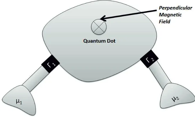
In nanosystems, one has control over their behavior through the changes of external parameters. Further, in the case of an open quantum dot (QD), a nanosystem of zero dimension, where the elec-trons enter and exit the dots through the leads, one has an analog computer of the compound nucleus, since resonances in the electron conductance are in general overlapping and resemble very much the behavior of complex chaotic systems. Other nanosystems of higher dimensions are fabricated and studied. Quantum wires have a dimension of 1, while graphene has a dimension of 2. In the follow-ing, we study the statistical properties of QDs, depicted in Fig. [1]. It consists of a chaotic quantum dot connected to two electron reservoirs via ideal leads with a number of open channels. Electron
C
Owned by the authors, published by EDP Sciences, 2014
This is an Open Access article distributed under the terms of the Creative Commons Attribution License 2.0, which permits unrestricted use, distribution, and reproduction in any medium, provided the original work is properly cited.
Figure 1.A schematic diagram showing a quantum dot coupled to two leads.
reservoirs have a temperatureT and electrochemical potentialsμ1 andμ2, generating a potential
dif-ferenceeV. The injected electrons have a finite probability of tunneling for entrance and exit due to the presence of barriersΓ1andΓ2. The QD can couple the spin and orbital degrees of freedom through
relativistic corrections owing to the band structure and/or asymmetries in interfaces of heterostrutures. There is an extensive literature devoted to the study of the statistical properties of the electronic conductance in ballistic open quantum dots containing a large number of electrons.[15] In such sys-tems, it is customary to assume that the underlying electronic dynamics is chaotic to statistically describe the electron transport properties using random matrix theory (RMT) [3–5] and the Landauer conductance formula[16, 17] Within this framework, the conductance fluctuations are universal func-tions that depend on the quantum dot symmetries, such as time-reversal, and on the number of open modes N connecting the QD to its source and drain reservoirs. In the semiclassical limit of large N, the statistical transmission fluctuations are accurately modeled by Gaussian processes. In practice, it has been experimentally observed [21] and theoretically explained [22] that, even for small values of N and at very low temperatures, dephasing quickly brings the QD conductance fluctuations close to the Gaussian limit. The electronic conductance in open ballistic QDs exhibits random fluctuations as an external parameter, such as a magnetic fieldBor an applied gate voltageVg, is varied. So far, the
2 Ericson Fluctuations
The average value of fluctuating quantities of a physical system are calculable with available theo-ries. This is the case of the average compound nucleus cross section, which is given by the Hauser-Feshbach theory. The same holds for open quantum dots. A more stringent measure of the nature of these fluctuating observables can be best quantified with the aid of the correlation function. The resulting function is Lorentzian in shape as demonstrated by Ericson [2]. Consider the conductance in QDs. It is given by the Landauer-Büttiker formula [16, 17],
G= 2e h T =
2e hTr(t
†t) (1)
whereT is the dimensionless conductance given in terms of the transmission matrix, which appears in the S-matrix as [20],
S=
r t
t r
(2)
The usual decomposition ofT into an average part plus a fluctuation part is made,
T =T+Tf l (3)
Then the correlation function is given by
C(δZ)=Tf l(Z+aδZ)Tf l(Z−bδZ), (4)
whereZcan be the energy or any other quantity that may modify the Hamiltonian. The above correla-tion funccorrela-tion does not depend on the choice ofaandb, provided thata+b=1. In nuclear physics the only quantity that is available for change and study is the energy. In QD, on the other hand, besides the energy, one may apply a magnetic field or change the shape, both of which are treated as exter-nal parameters. For the caseZ = E, the result of the average above is given by Ericson correlation function,
C(ε)= T
f lTf l
1+(εγ)2 (5)
In the case of a variation of an external parameter,X, Efetov [6, 7], has shown that the correlation function is a squared Lorentzian,
C(δX)= T
f lTf l
[1+(δXX c)
2]2 (6)
In the above equations, the averageTf lTf lis the variance. In the case of the compound nucleus,
this quantity is the square of the Hauser-Feshbach cross section. Further, if direct reactions are present, the generalized correlation function for the transition from channelcto channelcis then given by,
Ccc(ε)=
2σdccσccf l+(σccf l)2
1+(εγ)2 (7)
parameter having a more complicated structure. It has been proven thatγis related to the density of states of the system,ρ=1/D, , whereDis the average resonance spacing, through the formula,
γ= D
2πT rP (8)
wherePis the transmission probability (or the tunneling probability) matrix. This is usually calculated with the optical potential in the nuclear case. In the case of QD, theP’s are coefficients that are varied
externally. In the case ofP=1, we have the interesting sum rule for QD,
γ= D
2πN (9)
whereNis the number of open channels.
Through the above sum rule, one can determine the density of states, once the correlation analysis is performed andΓis extracted. A simple formula forXcis more difficult to obtain. However it can
be shown thatXcdepends on the number of open channels, asXc∼ √N
A general correlation function for QD can be derived in the case of a tunneling probability,Γ, smaller than one (all the above results assumeΓ =1). One finds [14], using the stub model [18],
C(ε)=Tf lTf l
3Γ(2−Γ)−2 1+(ε/Γ)2 +
4[1+ Γ(Γ−1)] [1+(ε/γ)2]2
(10)
and,
C(δX)=Tf lTf l
2Γ(1−Γ) 1+(δX/Xc)2 +
2+ Γ(3Γ−4) [1+(δX/Xc)2]2
(11)
The above correlation functions reduce to the ones in Eqs. (5) and (6), in the limit of fully open QDs. Further, the energy correlation function,C(ε) above exhibits an anti-correlation (negative cor-relation function). In fact, in the limit of very small tunneling (Γ→0), one has,
C(ε)=Tf lTf l 1−(ε/γ) 2
[1+(ε/γ)2]2 (12)
Ericson-type analysis has been extensively used in compound nuclear reaction studies. Further-more, it has been employed by researchers in other areas to characterize chaotic scattering systems in general, and has become an integral part of the theoretical investigation of complex chaotic systems.
3 Number of maxima method
The un-averaged cross section in compound nucleus reactions or electron conductance in QDs exhibits energy fluctuations that show the characteristics of noise. One may wonder whether something useful can be extracted from such a chaotic function. Since the underlying S-matrix is random in nature, one could trace some features of the fluctuating observable to this randomness. In the following we calculate the average density of maxima in the un-averaged, fluctuating, observable and show that it is directly related to the correlation function. This added information sheds more light on the nature of chaotic scattering systems.
The condition that the random observable has a maximum at energyEis,
We call,τ1=Tf l(E), τ2=Tf l(E+ε0), τ3=Tf l(E−ε0), with,
τ1> τ2> τ3. (14)
We now introduce the joint probability distribution of the three random numbers,τ1, τ2,andτ3. We
do this by first recalling the Gaussian distribution of a single variable,x,
P(x)= 1 2πx2
exp [−1 2
x2
x2] (15)
wherex2is the variance or second moment of the distribution,
x2=
∞
−∞x
2dxP(x) (16)
Of courseP(x) is normalized by construction,
∞
∞
dxP(x)=1. (17)
The above Gaussian distribution can be obtained from the principle of maximum information entropy subjected only to constraints given by conditions Eqs. (16, 17), namely,
δ S +λ1<x2>+λ2<1>
=0 (18)
where the information entropyS, is given by,
S =−
dxP(x) lnP(x). (19)
Performing the variational calculation of Eq. (19), we get,
[lnP+1+λ1x2+λ2]δP=0, (20)
which yields,
P(x)=e1−λ2exp [−λ1x2] (21)
The generalization of the above to the distribution of the components of a 3-vector is now straightfor-ward,
P(τ1, τ2, τ3)=
1
(2π)3/2D1/2 exp
−1
2X
TAX
, (22)
where the vectorXT =(τ1, τ2, τ3), is its transpose ofX, andD=detC, with C being the correlation
matrix, whosek jelement is just the S-matrix two point correlation function,
C=
⎛ ⎜⎜⎜⎜⎜
⎜⎜⎜⎝ ττ12ττ11 ττ12ττ22 ττ21ττ33 τ3τ1 τ3τ2 τ3τ3
⎞ ⎟⎟⎟⎟⎟
⎟⎟⎟⎠ (23)
Ck j=τkτj=| Tf l
1+i(k−j)ε0 γ
The matrixA = C−1. With the above, we can calculate the average number of maxima, through
integration over the three variables, under the constraint of Eq. (14),
ρE=
2
ε0
∞
−∞dτ2
τ2
−∞dτ1
τ1
−∞dτ3F(τ1, τ2, τ3) (25)
Integrating the above equation yields,
ρE=πε1
0
tan−1
4 C(0)−C(ε0)
C(0)−C(2ε0)
−1 (26)
Using the explicit form of the correlation function,C(ε)=(Tf l)2/(1+ε2/γ2), we get,
ρE=
1
πε0
tan−1
3 ε
2 0 γ2+ε2
0
(27)
In the limit ofε0 =0, the above relation reduces to,
ρE=
√
3
πγ =
0.55
γ (28)
Therefore, by counting the average number of maxima in theun-averagedcross section in a compound nucleus reaction, or in the electron conductance in a chaotic open QD, one obtains the correlation width, also obtainable from Ericson analysis of the correlation function, Eq. (5). This supplies a powerful double checking of the whole idea of statistical processes in quantum systems, namely being described by a random S-matrix.
The average density of maxima in the case of the external parameter variation, namely
C(δX)= T
f lTf l
[1+(δXX c)
2]2,
is
ρX=
3
π√2Xc
= 0.68
Xc (29)
The formulae for the average density of maxima can be cast in different forms if the condition for a maximum is changed into a condition on the first and second derivative of the fluctuating observable. Here one defines the maximum inTf l(Z) asTf l(Z)>0, andTf l(Z+δZ)<0, in the interval [Z,Z+δZ],
providedδZis sufficiently small. Expanding inδZ, the condition for a maximum is then,
−Tf l(Z)δZ >Tf l(Z)>0 (30)
The average density of maxima is then given by integrating the joint probability distribution,
P(T,T), over the random variables,T,T, subject to the above constraint.
0
−∞dT −T
0
dTP(T,T)=−δZ
0
−∞dT
TP(0,T)≡δZρZ (31)
An appropriate Gaussian distribution function for the the three assumed random variables,T,T,
C=
⎛ ⎜⎜⎜⎜⎜ ⎜⎜⎜⎝ |T|
2 0 T T
0 |T|2 0
TT 0 |T|2
⎞ ⎟⎟⎟⎟⎟
⎟⎟⎟⎠ (32)
is then constructed. The zero elements in the above correlation matrix are a direct consequence of the correlation function when expanded in powers ofδZ. In fact, the non-zero elements, are obtained from the CF as,
|T|2=− d2
d(δZ)2C(δZ)|δZ=0, (33)
T T= d 2
d(δZ)2C(δZ)|δZ=0, (34)
and
|T|2= d 4
d(δZ)4C(δZ)|δZ=0 (35)
.
The average density of maxima, Eq. (31), involves an integral of onlyTandT, and what we need at the end isP(0,T). This distribution is easily obtained fromP(T,T,T) by integrating over the redundant variableT, and settingT=0, getting
P(0,T)= 1 2π
1
[T]2 [T]2exp
−1
2 [T]2
[T]2
. (36)
One can then obtain the average density of maxima as,
ρ= 1 2π
|T|2
|T|2 (37)
The average density of maxima in the case of energy fluctuations, is then
ρE=
√
3
πγ (38)
and for the variation of the external parameter, where the correlation function is a squared Lorentzian,
ρX=
3
π√2Xc (39)
Equations, (38) and (39) coincides with Eqs. (28) and (28), attesting to the equivalence of the two manners of defining a maximum.
The above results are valid for open quantum dots. In the general case of partially open QD. where the tunneling probability (assumed to be equal for all the channels),Γ, is less than one the formulae for the average densities were recently derived [14], and they are given by,
ρE= √
3
πγ
9Γ2−18Γ +10
5Γ2−10Γ +6 (40)
ρX=
√
3
π√2Xc
7Γ2−10Γ +6
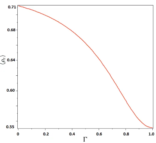
Figure 2.The figure shows the average density of maximum dependence on the tunneling rates for parametric variations of energy. Notice the asymptotically decreasing behavior up to the limiting value of 0.55 atΓ =1.
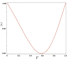
The dependence ofρEandρXonΓare exhibited in Figs. (2) and (3).
The above formulae reduce to the former ones in the completely open QD,Γ =1. In the opposite limit,Γ =0, we get,
ρE=
√
5
πγ (42)
Surprisingly, for the case of an external parameter variation, we obtain exactly the same result as in the caseΓ =1,
ρX=
3
π√2Xc
(43)
Clearly, in this latter case, there is a an extremum (minimum) in the dependence ofρXonΓ. This
happens forΓ∼0.6
4 Random matrix simulations
In this section we present the results of a random matrix simulation based on a random Hamiltonian based S-matrix used extensively by Weidenmüller and collaborators [3–5],
Figure 3. The figure shows the average density of maxima dependence on the tunneling rates for parametric variations of a magnetic field. Notice the presence of a minimum and the asymptotically equal values (atΓ=1.0, and 0.0).
member of the Gaussian orthogonal (unitary) ensemble for the symmetric (broken) time-reversal case. The matrixWof dimensionM×(N1+N2) contains the channel-resonance coupling matrix elements.
Specifically, for a QD in the chaotic universal regime, the eigenvaluesWofWW†are connected with the tunneling probabilityΓthrough the formula [15]W=MD(2−Γ±2√1−Γ)/(π2Γ). Since theH
matrix is statistically invariant under orthogonal or unitary transformations, the statistical properties ofS depend only on the mean resonance spacingD, determined byH, and onW†W.
We consider a non-ideal coupling (finite tunneling probabilities), i.e, an arbitrary interaction be-tween the open channels and long-range resonant modes of the QD. We separate the matrixW into blocks corresponding to the respective couplings of QD with the two leads,W = (W1,W2), where Wi is a M ×Ni matrix. We disregard the direct processes requiring the orthogonality condition
Wi†Wj = ωiMDδi j/π2 withωi = diag(ωi,1, ωi,2, . . . , ωi,Ni). The tunneling probability (barrier)Γi,c of the channelc and leadi can be written in terms of the diagonal matrixω through the relation Γi,c = sech2(τi,c/2) with τi,c = −ln(ωi,c). We consider equivalent couplings, Γi,c = Γi, symmetric
contacts, and a large number of resonances in the QD. Without loss of generality, we choose the pure unitary ensemble for numerical simulation of the previously mentioned Landauer-Büttiker conduc-tance CF (identified with the covariance ofT(ε) =Tr(t†(ε)t(ε))) using the transmission sub-matrix of Eq.(2 ), which can be written ast(ε) = −2πiW1†(ε−H+iπWW†)−1W2. The numerical
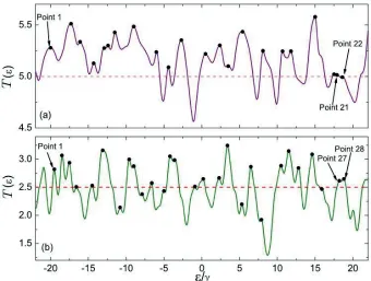
Figure 4.Typical dimensionless conductanceT as a function ofε/γforN=60 channels coupled to resonances through finite tunneling probabilities. The continuous lines indicate the numerical results for a single realization ofH, the dots indicate the maxima ofTand the dashed line is theε-independent conductance average.
nicely confirms an auto-correlation lengthγ=NΓD/(2π). The discrepancies are very small and stay within the statistical precisionNr−1/2.
We have verified the accuracy of our expressions for the average density of maxima by comparing them with a direct counting of these maxima in Fig.[1]. The results are very good. We have also con-firmed the accuracy of the expressions for the correlation functionsC(ε) andC(X) using the results of the random matrix simulations, Fig.[2]. Again, the results are very good, and confirm the correctness or our analytical results.
5 Discussion and conclusions
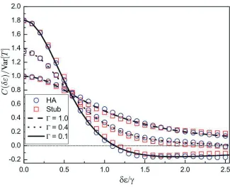
Figure 5. Correlation function (normalized covariance) as a function of a parametric variation of the energy showing a transition from a Lorentzian (long dashed line) to an anti-correlation (continuous line) as a function of the symmetric tunneling probabilityΓ. The labels "HA" and "stub" refer to results of simulations performed using the random Hamiltonian model of the S-matrix, Eq. (44), and the stub model of Ref. [18].
research. The limitΓ = 1 refers to overlapping resonances (strong absorption), whileΓ ∼0 corre-sponds to isolated resonances (weak absorption). In fact, Ref. [12] presented data for the reaction p +35Cl→α+32S that shows the anti-correlation effect. We are currently pursuing this line of research.
References
[1] W. Hauser and H. Feshbach, Phys. Rev.87, 366 (1952).
[2] T. Ericson, Phys. Rev. Lett.,5, 430 (1960), and T. Ericson, Ann. Phys. (NY),23, 390 (1963). [3] G. E. Mitchell, A. Richter, and H. A. Weidenmüller, Rev. Mod. Phys.,82, 2845 (2011). [4] J. J. M. Verbaarschot, H. A. Weidenmüller, and M. R. Zirnbauer, Phys. Rep.129, 129 (1985). [5] T. Guhr, A. Müller-Groeling, and H. A.Weidenmüller, Phys. Rep.299, 189 (1998).
[6] K. B. Efetov, Phys. Rev. Lett.,74, 2299 (1995).
[7] M. Martínez-Mares, C. H. Lewenkopf, and E. R. Mucciolo, Phys. Rev. B69, 085301 (2004). [8] R. O. Vallejos and C. H. Lewenkopf, J. Phys. A34, 2713 (2001)
[9] D. M. Brink and R. O. Stephen, Phys. Lett.,577 (1963).
[12] Y. Alhassid, Rev. Mod. Phys.,72, 895 (2000).
[13] J. G. G. S. Ramos, D. Bazeia, M. S. Hussein, and C. H. Lewenkopf, Phys. Rev. Lett.,107, 176807 (2011).
[14] A. L. R. Barbosa, M. S. Hussein, and J. G. G. S. Ramos, Phys. Rev. E88, 010901(R) (2013). [15] C. W. J. Beenakker, Rev. Mod. Phys.69, 731 (1997).
[16] R. Landauer, IBM Journal of Research and Development1, 223 (1957). [17] M. Büttiker, Phys. Rev. Lett.57, 1761 (1986).
[18] P. W. Brouwer, and C. W. J. Beenakker, J. Math. Phys.37, 4904 (1996).
[19] J. G. G. S. Ramos, A. L. R. Barbosa, and A. M. S. Macêdo, Phys. Rev. B84, 035453 (2011). [20] P. A. Mello and N. Kumar,Quantum transport in mesoscopic systems(Oxford University Press,
2004).
[21] A. G. Huibers, S. R. Patel, C. M. Marcus, P. W. Brouwer, C. I. Duruöz, and J. S. Harris, Phys. Rev. Lett.81, 1917 (1998)
[22] E. R. P. Alves and C. H. Lewenkopf, Phys. Rev. Lett.88, 256805 (2002). [23] B. Dietz, A. Richter, and H. A. Weidenmüller, Phys. Lett. B697, 313 (2011). [24] Y Ujiie et al., J. Phys. Condens. Matter21, 382202 (2009).
[25] F. V. Tikhonenko, A. A. Kozikov, A. K. Savchenko, and R. V. Gorbachev Phys. Rev. Lett.103, 226801 (2009).