FPGA Implementation of CORDIC Based DHT for Image Processing Applications

FPGA Implementation of CORDIC Based

DHT for Image Processing Applications

Shaik Waseem Ahmed

, Sudhakara Reddy.P

P.G. Student, Department of Electronics and Communication Engineering, SKIT College, Srikalahasti, India1

Associate Professor, Department of Electronics and Communication Engineering, SKIT College, Srikalahasti, India2

ABSTRACT: Digital image processing(DIP) is the use of computer algorithms to perform image processing on digital images. The basic operation performed by a simple digital camera is, to convert the light energy to electrical energy, then the energy is converted to digital format and a compression algorithm is used to reduce memory requirement for storing the image. This compression algorithm is frequently called for capturing and storing the images. This leads us to develop an efficient compression algorithm which will give the same result as that of the existing algorithms with low power consumption. Image compression is useful as it helps in reduction of the usage of expensive resources, such as memory, or the transmission bandwidth required. But on the downside, compression techniques result in distortion and also additional computational resources are required for compression-decompression of the medical image data.

In this, we proposed DHT based image compression technique. The computational complexity is further reduced by

using pipelined CORDIC architecture for computation of sin and cos terms in DHT. The CORDIC based DHT is

partially simulated and synthesized by using Xilinx ISE design suite and the same was implemented on targeted FPGA. The hardware requirements and gate delay values are observed and noted down.

KEYWORDS: CORDIC, DHT, FPGA, Image Processing.

I. INTRODUCTION

Compression, the art and science of reducing the amount of data required to represent an image, is one of the most useful and commercially successful technologies in the field of digital image processing. Digital image and video compression is now very essential. Bio-Medical Image Compression would not be feasible unless a high degree of compression is achieved. Compression is useful as it helps in reduction of the usage of expensive resources, such as memory ( hard disks), or the transmission bandwidth required. In today’s Age of competition where everything is reducing its size every minute, the smaller is the better. But on the downside, compression techniques result in distortion and also additional computational resources are required for compression-decompression of the data. Compression ratio (C) is defined as the ratio of the size of compressed data to that of the uncompressed data.

𝐶 = 𝑠𝑖𝑧𝑒 𝑜𝑓 𝑐𝑜𝑚𝑝𝑟𝑒𝑠𝑠𝑒𝑑 𝑑𝑎𝑡𝑎

𝑠𝑖𝑧𝑒 𝑜𝑓 𝑢𝑛𝑐𝑜𝑚𝑝𝑟𝑒𝑠𝑠𝑒𝑑 𝑑𝑎𝑡𝑎 (1) Redundancy is the reduction in size in comparison of the uncompressed size.

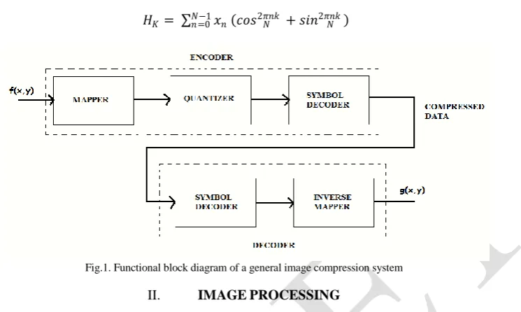
𝑅 = 1 – 𝐶 (2) In image compression process the image 𝑓(𝑥, 𝑦) is mapped to a format to reduce spatial redundancy. The Discrete Hartley transform is used for mapping Next quantization is done, where the loss of information takes place. Since it is an irreversible process, we can omit this step for a lossless coding technique. The final step is symbol coding, where various coding techniques can be used to represent the information in minimum possible number of bits[1] This is shown in figure 1.

The discrete Hartley transform is a linear, invertible function 𝐻: 𝑹 → 𝑹 (where R denotes the set of real numbers).

𝐻𝐾= 𝑁−1𝑛=0𝑥𝑛 𝑐𝑜𝑠 𝑁2𝜋𝑛𝑘 + 𝑠𝑖𝑛 𝑁2𝜋𝑛𝑘 (3)

Fig.1. Functional block diagram of a general image compression system

II. IMAGEPROCESSING

Image processing involves minimizing the size in bytes of a graphics file without degrading the quality of the image to an unacceptable level. The reduction in file size allows more images to be stored in a given amount of disk or memory space. It also reduces the time and bandwidth required for images to be sent over the Internet or downloaded from Web pages.

There are several different ways in which image files can be compressed. For Internet use, the two most common compressed graphic image formats are the JPEG format and the GIF for mat. The JPEG method is more often used for photographs, while the GIF method is commonly used for line art and other images in which geometric shapes are relatively simple.

The steps involved in image compression are as follows:

1. First of all the image is divided into blocks of 8x8 pixel values. These blocks are then fed to the encoder from

where we obtain the compressed image.

2. The next step is mapping of the pixel intensity value to another domain. The mapper transforms

images into a (usually non- visual) format designed to reduce spatial and

3. Temporal redundancy. It can be done by applying various transforms to the images. Here discrete Hartley

transform is applied to the 8x8 blocks.

4. Quantizing the transformed coefficients results in the loss of irrelevant information for the specified

purpose.

5. Source coding is the process of encoding information using fewer bits (or other information- bearing

units) than an unencoded representation would use, through use of specific encoding schemes.

Fig .2. Energy quantization based image compression encoder

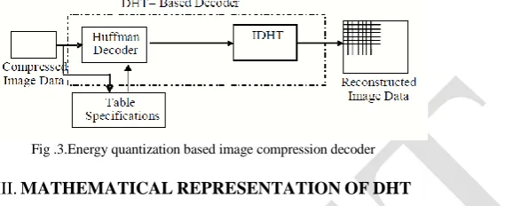
decoder. Next inverse transform (IDHT) is calculated to get the 8x8 blocks. These blocks are then connected to form the final image. From the reconstructed image pixel values it is clear that some of the high frequency components are preserved. This indicates that the edge property of the image is preserved.

Fig .3.Energy quantization based image compression decoder

III.MATHEMATICALREPRESENTATIONOFDHT

The Hartley transform is an integral transform closely related to the Fourier transform, but which transforms real- valued functions to real-valued functions. It was proposed as an alternative to the Fourier transform by R. V. L. Hartley in 1942. Compared to the Fourier transform, the Hartley transform has the advantages of transforming real functions to real functions and of being its own inverse. The discrete version of the transform, the Discrete Hartley transform, was introduced by R. N. Bracewell in 1983. Discrete Hartley Transform is the real valued transform which gives only real transform coefficients for real input stream. It has the main advantage over DCT of reducing the memory content up to 50% since the inverse transform is identical to the forward transform. Also, it retains the higher frequency components, which restores the detailing of the image. Since it is a real valued function unlike DFT, the computational complexities are also lower than in DFT algorithms [2].

Formally, the discrete Hartley transform is a linear, invertible function 𝐻: 𝑹 → 𝑹 (where 𝑹 denotes the set of real

numbers). The 𝑁 real numbers 𝑥0𝑥1. . . 𝑥𝑁−1 are transformed into 𝑁 real numbers 𝐻0𝐻1. . . 𝐻𝑁−1 according to the formula:

for 𝑘 = 0, 1 … 𝑁 − 1

𝐻𝐾 = 𝑁−1𝑛=0𝑥𝑛 𝑐𝑜𝑠 𝑁2𝜋𝑛𝑘 + 𝑠𝑖𝑛 𝑁2𝜋𝑛𝑘 (4) The inverse transform is given by: for 𝑛 = 0,1 … 𝑁 − 1

𝑥𝑛 = 1

𝑁 𝐻𝑛

𝑁−1

𝑘=0 𝑐𝑜𝑠 𝑁2𝜋𝑛𝑘 + 𝑠𝑖𝑛 𝑁2𝜋𝑛𝑘 (5) The cas function is given by:

𝑐𝑎𝑠 𝑁2𝜋𝑛𝑘 = 𝑐𝑜𝑠 𝑁2𝜋𝑛𝑘 + 𝑠𝑖𝑛 𝑁2𝜋𝑛𝑘 (6) and one of the properties of cas function is:

2𝑐𝑎𝑠(𝑎 + 𝑏) = 𝑐𝑎𝑠(𝑎)𝑐𝑎𝑠(𝑏) + 𝑐𝑎𝑠(−𝑎)𝑐𝑎𝑠(𝑏) + 𝑐𝑎𝑠(𝑎)𝑐𝑎𝑠(−𝑏) − 𝑐𝑎𝑠(−𝑎)𝑐𝑎𝑠(−𝑏) (7) 2 –Dimensional DHT of an array 𝑥 (𝑚, 𝑛) of size MxN may be defined as:

X k, l = M

m=0 Nn=0 x m, n cas(

2πmk

m +

2πnl

n ) (8) For 𝑘 = 0,1 … 𝑀 − 1 & 1 = 0,1 … 𝑁 − 1

The inverse transform is given by the same formula along with a scaling factor of 1/𝑀𝑁 i.e. 𝑋 𝑘, 𝑙 = 1

𝑀𝑁 𝑀

𝑚 =0 𝑁𝑛=0 𝑥 𝑚, 𝑛 𝑐𝑎𝑠(

2𝜋𝑚𝑘

𝑚 +

2𝜋𝑛𝑙

𝑛 ) (9) for 𝑘 = 0, 1 … 𝑀 − 1 & 𝑙 = 0,1 … . . 𝑁 − 1

The real and imaginary parts of the Fourier transform are given by the even and odd parts of the Hartley transform, respectively

𝐹 𝑊 =𝐻 𝑤 +𝐻(−𝑤 )

2 −

𝑖(𝐻 𝑤 −𝐻(−𝑤 ))

2 (10)

There is also an analogue of the convolution theorem for the Hartley transform. If two functions 𝑥 ( 𝑡 ) and

𝑦 ( 𝑡 ) have Hartley transforms𝑋 ( ) 𝑎𝑛𝑑 𝑌 ( ), respectively, then their convolution 𝑧 ( 𝑡 ) = 𝑥 ∗ 𝑦 has the Hartley transform:

𝑍 𝑤 = 𝐻 𝑥 ∗ 𝑦 = 2𝑝𝑖 (𝑋 𝑤 𝑌 𝑤 +𝑌 −𝑤 +𝑋(−𝑤 [𝑌 𝑤 −𝑌(−𝑤 )])

2 (11)

IV.8-POINT DHT SIGNAL FLOW

The signal-flow graph for 8- point DHT with pipelined stages with delays is shown in figure.4. The DHT of a real-

valued-point input vector𝑥0𝑥1. . . 𝑥𝑁−1, may be defined as

𝑋𝑘= 𝑁−1𝑛=0𝑥𝑛𝐶𝑁(𝑘, 𝑛) (12)

Where 𝐶𝑁 𝑘, 𝑛 = 𝑐𝑎𝑠 2𝜋𝑛𝑘 𝑁 = 𝑐𝑜𝑠 2𝜋𝑛𝑘 𝑁 + 𝑠𝑖𝑛 2𝜋𝑛𝑘 𝑁 (13)

for 𝑘, 𝑛 = 0,1 … . 𝑁 − 1 , Supposing 𝑁 to be an even number, the sequence 𝑥𝑛 is divided into two sub-sequences 𝑥1 and 𝑥2 length 𝑁/2 each, such that 𝑥1= {𝑥0, 𝑥2… . 𝑥𝑁−2} contains all even-indexed terms and 𝑥2= {𝑥1, 𝑥3… . 𝑥𝑁−1} contains all odd-indexed terms of the input sequence 𝑥. Then the DHT can be defined as: 𝑋𝑘 = 𝑥1𝐶𝑁 𝑘, 2𝑛 + 𝑥2𝐶𝑁(𝑘, 2𝑛 + 1) 𝑁 2−1 𝑛=0 𝑁 2−1 𝑛=0 (14)

Let 𝑋1𝑘 and 𝑋2𝑘 represent the (𝑁/2) –point DHT coefficients of sequences 𝑥1 and 𝑥2 of length (N/2) respectively. Using the symmetry properties of sine and cosine functions, the N-point DHT may be expressed as the following set of equations: 𝑋𝑘= 𝑋1𝑘+ 𝐸𝑘 (15)

𝑋𝑚 +𝑘 = 𝑋1𝑘− 𝐸𝑘 (16)

𝐸𝑘= 𝑋2𝑘cos 𝜋𝑘 𝑀 + 𝑋2 𝑀−𝑘 𝑠𝑖𝑛( 𝜋𝑘 𝑀) (17)

For 𝑘 = 1, 2 … 𝑀 − 1 where 𝑀 =𝑁 2.Hence for computing 8-point DHT from 4-point DHT the set of equations are shown in equations 18 to 25, which are obtained from equation 17 1. 𝑋0= 𝑋10+ 𝑋20 (18)

2. 𝑋1= 𝑋11+ (𝑋21+ 𝑋23)/ 2 (19)

3. 𝑋2= 𝑋12+ 𝑋22 (20)

4. 𝑋3= 𝑋13+ (𝑋21− 𝑋23)/ 2 (21)

5. 𝑋4= 𝑋10− 𝑋20 (22)

6. 𝑋5= 𝑋11− (𝑋21+ 𝑋23)/ 2 (23)

7. 𝑋6= 𝑋12− 𝑋22 (24)

8. 𝑋7= 𝑋13− (𝑋21− 𝑋23)/ 2 (25)

Fig.4. Flow chart of the 8-point DHT in pipelined approach with delays

adders perform the addition. It computes DHT in 5 pipelined stages. For first two stages, it consists of two 4-pointDHT

modules that receive the odd and even indexed subsequence 𝑥1 and 𝑥2 and from the input buffer. In the third pipelined

stage, multiplication with 1/ 2 is done for the required coefficients i.e. 𝑋21 𝑎𝑛𝑑 𝑋23. Next they are added and

subtracted in the fourth stage. During 3𝑟𝑑 _{and 4}𝑡𝑕 _{stages the rest of the coefficients are passed through a delay. Delay}

consists of simply registers i.e. they are stored in different registers and passed to the next stage. Finally the fifth pipelined stage is a parallel adder block which adds/subtracts the coefficients to give the desire output.[3] The block diagram of the described method is given in figure 2.

V. CORDICBASEDDHT

The CORDIC means Coordinate Rotation Digital Computer. CORDIC use simple shift and add operations for several computing tasks. It is generally faster than the other approaches when no hardware multiplier is available. In recent years, the CORDIC algorithms have been in use extensively for various applications, especially in FPGA implementation. The CORDIC provide an iterative solutions to perform vector rotations by arbitrary angles using only

shifts and adds. The CORDIC algorithm can be operated in either vectoring mode or rotation mode.[4]

Generalization of the CORDIC algorithm: The generalized CORDIC is formulated as follows

𝑥𝑖+1= 𝑥𝑖− 𝑚𝜎𝑖. 2−𝑖. 𝑦𝑖 (26)

𝑦𝑖+1= 𝑦𝑖+ 𝜎𝑖. 2−𝑖. 𝑥𝑖 (27)

𝑧𝑖+1= 𝑧𝑖− 𝜎𝑖. 𝛼𝑖 (28)

Where

𝜎𝑖 =

𝑠𝑖𝑔𝑛 𝑧𝑖 𝑓𝑜𝑟 𝑟𝑜𝑡𝑎𝑡𝑖𝑜𝑛 𝑚𝑜𝑑𝑒

−𝑠𝑖𝑔𝑛 𝑦𝑖 𝑓𝑜𝑟 𝑣𝑒𝑐𝑡𝑜𝑟𝑖𝑛𝑔 𝑚𝑜𝑑𝑒

(29)

For m= 1,0 or -1 which is suitable to perform rotations in circular , hyperbolic & linear coordinate system and α represents the angle. We have proposed an 8-point CORDIC based DHT with six CORDIC rotations to realize multiplier less approximation. They are circular rotation mode, circular vectoring mode, linear rotation mode, linear vectoring mode, hyperbolic rotation mode and hyperbolic vectoring mode

The CORDIC is hardware-efficient algorithms for computation of trigonometric and other elementary functions that use only shift and add to perform. The CORDIC set of algorithms for the computation of trigonometric functions was designed by Jack E. Volder in 1959 Later, J. Walther in 1971 extended the CORDIC scheme to other functions. Depending on the configuration, the resulting module implements pipelined parallel-pipelined, word-serial, or bit-serial architecture in one of two modes: rotation or vectoring. In rotation mode, the CORDIC rotates a vector by a certain angle. This mode is used to convert polar to Cartesian coordinates. For eg consider the multiplication of two complex

numbers 𝑥 + 𝑗𝑦 and (𝑐𝑜𝑠()  𝑗 𝑠𝑖𝑛()) .The result 𝑢 + 𝑗𝑣, can be obtained by calculating the final coordinate after

rotating a 2x2 vector [x y]T through an angle ( ) and then scaled by a factor r. This is achieved in CORDIC via a

three-stair procedure: angle conversion, Vector rotation and scaling. The radix 2 system is taken because it avoids the use of multiplications while implementing the above equation. Hence a CORDIC iteration can be realized using shifters and adders only.

The figure 5 shows the structure of a processing element which implements one CORDIC iteration the rotation mode and vectoring mode are two schemes for the CORDIC algorithm. In rotation mode, the aim is to rotate the given input

vector (𝑥 , 𝑦)𝑡 with a given angle. After n no’s of iterations, 𝑍𝑛 is driven to zero and the total accumulated rotation

angle is equal to desired angle Parallel pipelined architecture for CORDIC represents a version of the sequential CORDIC algorithm. Instead of reusing the same hardware for all iteration stages, the parallel architecture provides a separate processor for every iteration.

Fig.6. Parallel pipelined architecture for CORDIC

An example of the parallel CORDIC architecture for rotation mode is shown in figure 6. Each of the n processors present in the block performs a specific iteration, and a particular processor always performs the same iteration. All the shifters perform the fixed shift, so that it can be implemented in FPGA.[5] Every processor utilizes a individual arc tan value that can also be hardwired to the input of every angle accumulator in the absence of a state machine which provides simplicity to this type of architecture. The parallel architecture is much faster than the sequential architecture described in the “iterative Word-serial architecture” in figure 6. It takes new input data and puts out the results at every clock cycle, introducing a latency of n clock cycles. The architecture which is used in the design of the DHT is this parallel-pipelined architecture because this architecture which provides high throughput and low power consumption. Then we can apply the above conditions to the DHT equation.

The DHT is given

𝐻𝐾 = 𝑁−1𝑛=0𝑥𝑛 𝑐𝑜𝑠 𝑁2𝛱𝑛𝑘 + 𝑠𝑖𝑛 𝑁2𝛱𝑛𝑘 , 𝑘 = 0, 1 … 𝑁 − 1 (30) In this equation we have we have one multiplication and adder.

The equation (30) can be implemented by CORDIC as follows. In order to compute the 𝑐𝑎𝑠𝜃 term makes the initial

condition 𝑥𝑖𝑛 = 1/𝑘𝑚 , 𝑦𝑖𝑛 = 0 and 𝑧𝑖𝑛 = 𝜃. In this block diagram apply the above condition we get the 𝐶𝑎𝑠𝜃 term

as shown in figure 7.

𝑥[𝑛] Multiplied with 𝜃 , and its summation according to above equation are shown figure 8.

Fig.8. Block diagram of a N-bit adder

VI. RESULTSANALYSISANDIMPLEMENTATION

The real and imaginary parts of the Fourier transform are given by the even and odd parts of the Hartley transform, respectively

𝐹 𝑊 =𝐻 𝑤 +𝐻(−𝑤 )

2 −

𝑖(𝐻 𝑤 −𝐻(−𝑤 ))

2 (31)

There is also an analogue of the convolution theorem for the Hartley transform. If two functions 𝑥 ( 𝑡 ) and

𝑦 ( 𝑡 ) have Hartley transforms 𝑋 ( ) and 𝑌 ( ), respectively, then their convolution 𝑧 ( 𝑡 ) = 𝑥 ∗ 𝑦 has the Hartley transform:

𝑍 𝑤 = 𝐻 𝑥 ∗ 𝑦 = 2𝑝𝑖 (𝑋 𝑤 𝑌 𝑤 +𝑌 −𝑤 +𝑋(−𝑤 [𝑌 𝑤 −𝑌(−𝑤 )])

2 (32)

Similar to the Fourier transform, the Hartley transform of an even/odd function is even/odd, respectively. Hence DHT is a better option for compression algorithms and is used for mapping the input image pixels and quantization Normally the performance of a data compression scheme can be measured in terms of three parameters. These are Compression efficiency, Complexity and Distortion measurement for lossy compression. The Mean square error for a 1-D DHT data is given by:

𝑀𝑆𝐸 =1

𝑁 ⃓𝑥(𝑛)

𝑁−1

𝑛=0 − 𝑥′(𝑛)⃓ 2 (33) Where N is the number of pixels in the image, x (n) is the original data and x '(n) is the compressed data. The Peak Signal to Noise ratio (PSNR) is given by:

𝑃𝑆𝑁10𝑙𝑜𝑔 10255 2

𝑀𝑆𝐸′ (34) Where MSE is calculated for 2-D block as:

𝑀𝑆𝐸′= 1

𝑀𝑁 ⃓ 𝑥(𝑚, 𝑛)

𝑁−1 𝑛=0 𝑀−1

𝑚 =0 − 𝑥′(𝑚, 𝑛)⃓ 2 (35)

Fig 9 Simulation results

VII. CONCLUSION

In the present work, Discrete Hartley Transform for input matrix was implemented in FPGA using VHDL as the synthesis tool. The DHT was also calculated for 8-point input using two algorithms and their effectiveness were discussed, this primarily focuses on image compression with less computation and low power. The simulation results and design summary of DHT was obtained and it was shown that the architecture implemented is an efficient method which uses limited space and time. The hardware utilization is quite optimum and power analysis shows that the power requirement is also optimum. However if the input contents are large, they tend to overflow from the registers and hence error occurs. It can be rectified by saving the transformed coefficients in larger registers. Also due to quantization in the contents of the ROM, even-number outputs are more deviated from the desired results than the odd-numbered outputs.

REFERENCES

[1] S.K.Pattanaik and K.K.Mahapatra, “DHT Based JPEG Image Compression Using a Novel Energy Quantization Method” IEEE International conference on industrial technology, pp. 2827 – 2832, Dec 2006.

[2] RN.Bracewell, 0.Buneman, H. Hao and J. Villasenor, “Fast two-dimensional hartley transform” Proceedings of IEEE, Vol 74, No. 9, Sept1986. [3 ] C. H. Paik and M. D. Fox, “Fast Hartley transform for image processing,” IEEE Trans. Med. Image, vol. 7 , no. 6, pp. 149–153, Jun. 1988 [4 ] P.K.Meher, S. Thambipillai and J.C. Patra, “Scalable and modular memory-based systolic architectures for discrete hartley transform” IEEE Transactions on circuits and systems-I: regular papers, Vol53, pp. 1065-1077, May 2006

[5] A. Amira, “An FPGA based system for discrete hartley transforms. “IEEE publication, pp. 137-140, 2003 [6] R.C. Gonzalez, R.E. Woods, Digital Image Processing, Pearson Education 3rd Edition 2008

[7] CR. Baugh and BA. Wooley, “A two’s complement parallel array multiplication algorithm” IEEE Transactions on computers, Vol C-22, pp. 1045- 1047, Dec 1973

[8] Bracewell, Ronald N. “The Hartley transform” New York: Oxford university press 1986 [9] Ranjan Bose, Information theory coding and Cryptography, Tata McGraw-Hill 2003.

[10] F.Vahid and T. Givargis, Embedded system design: A unified hardware/software introduction, Wiley India (P.) Ltd, 3 𝑟𝑑_{edition 2009.} [11] H.S. Hou, “The fast Hartley transform algorithm,” IEEE Transactions on Computers, vol. C-36, no. 2, pp. 147–156, Feb. 1987.

[12] L.W. Chang and S.W. Lee, “Systolic arrays for the discrete Hartley transform,” IEEE Transactions Signal Processing, vol. 39, no. 11, pp. 2411– 2418, Nov. 1991.