over Prime Fields by Efficiently Computable
Formulas
Saud Al Musa and Guangwu Xu?
Department of EE & CS, University of Wisconsin-Milwaukee, USA,
{salmusa,gxu4uwm}@uwm.edu
Abstract. This paper addresses fast scalar multiplication for elliptic curves over finite fields. In the first part of the paper, we obtain sev-eral efficiently computable formulas for basic elliptic curves arithmetic in the family of twisted Edwards curves over prime fields. Our 2Q+P
formula saves about 2.8 field multiplications, and our 5P formula saves about 4.2 field multiplications in standard projective coordinate systems, compared to the latest existing results. In the second part of the paper, we formulate bucket methods for the DAG-based and the tree-based ab-stract ideas. We propose systematically finding a near optimal chain for multi-base number systems (MBNS). These proposed bucket methods take significantly less time to find a near optimal chain, compared to an optimal chain. We conducted extensive experiments to compare the per-formance of the MBNS methods (e.g., greedy, ternary/binary, multi-base NAF, tree-based, rDAG-based, and bucket). Our proposed formulas were integrated in these methods. Our results show our work have an impor-tant role in advancing the efficiency of scalar multiplication.
Keywords: twisted Edwards curves, Edwards curves, scalar multiplication, ef-ficient formulas, DBNS, MBNS
1
Introduction
Elliptic curve cryptography (ECC) is a type of public key cryptography that was initially introduced by Koblitz and Miller [22, 32]. ECC has an efficiency advantage over other public key cryptographies. For instance, a key length of 283-bit in ECC is regarded as secure as 3072-283-bit in RSA public key cryptography [25]. Scalar multiplication (tP) is the most expensive ECC operation that is extensively used in cryptographic protocols. It is an operation that adds P to itself t times such that tP =P+P+...+P
| {z }
t times
where P is a point on an elliptic
?Research supported in part by the National Key Research and Development Program
curve over finite fields and t is a large positive integer. Scalar multiplication efficiency in our framework relies on the method (e.g., binary, NAF) and the cost of formulas (e.g., point doubling (2P), point addition (P +Q)). The cost of 2P andP +Qformulas varies in different coordinate systems over different finite fields.
We express the cost of formulas by the number of field inversions (I), mul-tiplications (M), and squarings (S). We discuss a class of specific curves over prime fields called twisted Edwards curvesEa,d, as represented by Equation (1) and Equation (3). We express the notationsMa orMd to represent field multi-plication with one of the multiplicands to be twisted Edwards curves coefficient aor d. Addition/subtraction operations are ignored since they are cheap oper-ations over both prime and binary fields. We express the conjugate ofT by ¯T. To obtain the conjugate of a binomial, we need to change the sign between the two terms. For example, letT =Y +X. Then ¯T =Y −X.
We use the squaring to multiplication (S/M) ratio to measure the squaring cost. This is because the S/M ratio varies in different devices over different finite fields. The cost of one squaring operation is less than or equal to one multiplication operation. For prime fields, theS/M ratio is a high ratio and it is closer to one. For binary fields, it is a low ratio and the squaring is closer to a free operation [19, 8]. To simplify the comparison over prime fields, we assume 1S = 0.8M, Md = 1M, and Ma is a free operation as will be seen later, a is usually a small number. An inversion operation is more expensive than a multiplication operation over both binary and prime fields. We use the inversion to multiplication (I/M) ratio to measure the inversion cost. TheI/Mratio also varies in different devices over different finite fields [19, 8].
One technique to speed up scalar multiplication is to use projective coordi-nate systems. When we use projective coordicoordi-nates, we avoid inversion operations completely. First, we convert an affine point to a projective point. Then, we per-form scalar multiplication without any inversion operations. Lastly, we reverse a projective point to an affine point. The cost of converting an affine point to a projective point or vice versa is very minor in comparison to the cost of a scalar multiplication operation. As a result, the number of operations can be significantly reduced, especially for a high I/M ratio device. For this reason, numerous studies proposed projective coordinate systems for different elliptic curves [2, 5, 35, 24, 23, 20]. For Weierstrass curves over prime fields, Jacobian co-ordinates in our framework are the most efficient projective coco-ordinates [20]. For twisted Edwards curves over prime fields, standard projective coordinates in our framework are the most efficient projective coordinates [2].
Another technique to speed up scalar multiplication is to use double-base number system (DBNS) forms [13]. Integer t is represented in the DBNS in the form of t =
l P
i=1
multiplication since point addition is an expensive operation in comparison to other formulas. Multi-base number system (MBNS) is a natural extension of the DBNS [33]. When integer t is represented in the MBNS, the number of point additions continues to minimize.
The MBNS requires optimized point tripling (3P) and point quintupling (5P) formulas to be fast and practical. Therefore, numerous studies proposed optimized 3P and 5P formulas in different elliptic curves over different finite fields. The state of the art 3P and 5P formulas are described as follows. For Weierstrass curves, Yu, Kim, and Jo derived 3P formulas in affine coordinates over both binary and prime fields [38]. Longa and Miri derived a 3P formula and Giorgi, Imbert, and Izard derived a 5P formula in Jacobian projective coordi-nates over prime fields [28, 17]. Al Musa and Xu derived 3P and 5P formulas in λ-projective coordinates over binary fields [1]. For twisted Edwards curves over prime fields, Bernstein, Chuengsatiansup, and Lange derived a 3P formula and Li, Yu, and Wang derived a 5P formula in standard projective coordinates [4, 26].
For efficiency reasons, when integert is represented in the DBNS, it has to be represented as a double-base chain. In a double-base chain, the sequence of the exponents ai and bi decreases. Therefore, other studies proposed methods that convert integer t to a double-base chain. Dimitrov, Imbert, and Mishra proposed the greedy method [11]. Ciet, Joye, Lauter, and Montgomery proposed the ternary/binary method [9]. Longa and Gebotys proposed the multi-base NAF method [27]. Doche and Habsieger proposed the tree-based method [15]. Bernstein et al. proposed the rDAG-based method [4]. These methods can be extended to convert integert to a multi-base chain [33, 39].
1.1 Our Contribution
In this paper, we consider the efficiency problem of scalar multiplication for el-liptic curve cryptography and present three main contributions. The first part of our contribution is to derive formulas for twisted Edwards curves. We derive 2Q+P and 5P formulas in standard twisted Edwards coordinate systems over prime fields. To the best of our knowledge, our 2Q+P is the first proposed dedicated formula for twisted Edwards curves. It saves 1M+ 1Md+ 1Ma+ 1S
≈2.8Min comparison to a non-dedicated formula. It saves 3Sin comparison to 2Q+Pin Jacobian Weierstrass (a=−3) coordinates. Our 5Pformula costs 15M + 1Ma + 3S≈17.4M. It saves 4.2M in comparison to the state of the art 5P formula [26]. It saves approximately 2Min comparison to 5Pin Jacobian Weier-strass (a=−3) coordinates. We also improve the P+Q formula by using the pre-computation concept. This proposedP +Q formula with pre-computation saves 1Md + 1Ma ≈1Mover theP+Qformula without pre-computation.
are the first study that proposes systematically finding a near optimal chain for the MBNS methods. Moreover, these proposed methods show that the tree-based method is far from producing a near optimal chain.
The third part of our contribution is to conduct experimental comparison between the MBNS and the NAF methods. We utilize our formulas in these MBNS methods. The investigated MBNS methods are greedy, ternary/binary, multi-base NAF, tree-based, rDAG-based, and bucket methods. We use three types of measurements to compare the methods: the chain length, the chain cost, and the running time. The running time takes into consideration the conversion cost. Other experimental results in [4, 9, 11, 15, 27] were conducted without con-sidering the running converting time. Our experimental results show that the MBNS methods without pre-computation had an approximately 12% to 16% lower average chain cost in comparison to the NAF method. Except for the greedy method, they gave an approximately 12% to 18% faster average running time. They also show that the chain cost could be further improved if the MBNS methods with pre-computation were considered. However, this pre-computation could lead to extra time to find the chain.
1.2 ECC Applications
ECC is appropriate for an application that requires higher security and efficien-cy. One application for ECC is the Internet of Things (IoT). IoT can be seen as many embedded systems and sensors connected through an insecure chan-nel. These embedded systems and sensors have restricted resource capabilities. For example, He and Zeadally suggested ECC authentication schemes for radio-frequency identification (RFID) chips [21]. This is because ECC is more efficient for the computing resources than other public-key cryptographic systems. An-other practical application for ECC is within a blockchain. The blockchain is formed from distributed systems that work together to verify transactions [10]. For example, Bitcoin blockchain uses ECC digital signature schemes to verify digital currency transactions [34]. In addtion, computer network protocols use ECC in key agreement and digital signature schemes. For example, the latest version of the Transport Layer Security (TLS 1.3) protocol includes ECC in the supported cipher suite list [36].
The rest of the paper is organized into five sections. The proposed 2Q+P and 5Pformulas are presented in Section 2. In Section 3, we introduce the MBNS and proposed the bucket methods. In Section 4, we conducted experiments to com-pare the performance of the MBNS methods with and without pre-computation. Finally, we conclude our work in Section 5.
2
Twisted Edwards Curves
Bernstein, Birkner, Joye, Lange, and Peters introduced twisted Edwards curves over prime fieldsFp [2]. Twisted Edwards curvesEa,d are represented by
where a, d∈Fp, p >3 is a prime number,a6=dand a, d6= 0. The denotation Ea,d(Fp) is the set of all points (x, y) where x, y ∈ Fp that satisfies the above equation.Ea,d(Fp) is an abelian group under the point addition operation. The identity point for the group is the point (0,1). The negative of pointP= (x, y)∈
Ea,d(Fp) is another point−P = (−x, y)∈Ea,d(Fp).Ea,d has a unified formula for bothP+Qand 2P. LetP = (x1, y1)∈Ea,d(Fp) andQ= (x2, y2)∈Ea,d(Fp). ThenP+Q= (x3, y3)∈Ea,d(Fp) can be computed by
x3=
x1y2+y1x2 1 +dx1y1x2y2 y3=
y1y2−ax1x2 1−dx1y1x2y2
.
Edwards curves are a special class of twisted Edwards curves. Edwards curves Ed are represented by
Ed:x2+y2= 1 +dx2y2 (2)
where d∈ Fp andd 6={0,1}. In other words, Edwards curves are twisted Ed-wards curves with the coefficienta= 1 [6, 5].
2.1 Standard Projective Coordinates
Bernstein et al. also introduced two main representations for twisted Edwards curves in projective coordinates: standard twisted Edwards coordinates and in-verted twisted Edwards coordinates [2]. A projective point in standard twisted Edwards coordinates is represented as (X, Y, Z). An affine point can be convert-ed to projective point by using the relation (X, Y, Z) = (x, y,1). A projective point can be converted to an affine point by using the relation (x, y) = (XZ,YZ) where Z 6= 0. The curve equation in standard twisted Edwards coordinates is represented by
(aX2+Y2)Z2=Z4+dX2Y2. (3) 2P in standard twisted Edwards coordinates saves 1Mdin comparison to 2P in inverted twisted Edwards coordinates. It saves approximately 0.8Min com-parison to 2P in Jacobian Weierstrass coordinates (a=−3), as Table 1 shows. In our framework of scalar multiplication methods, 2P is used more frequently than other formulas (e.g., P +Q, 3P). Therefore, 2P has a greater impact on the performance than other formulas. As a result, more efforts were made to derive efficient formulas in standard twisted Edwards coordinates and this is the reason we derive efficient formulas in standard twisted Edwards coordinates.
2.2 A Proposed P +Q Formula
Table 1.The Cost of Efficient Formulas in Twisted Edwards and Jacobian Weierstrass Coordinates overFp
Standard twisted Edwards (a= 1) Jacobian Weierstrass (a=−3) MixedP+Q 9M+ 1S≈9.8M(this work) 7M+ 4S≈10.2M[28]
P+Q 10M+ 1S≈10.8M(this work) 11M+ 5S≈15M[28]
2P 3M+ 4S≈6.2M[2] 3M+ 5S≈7M[28]
3P 9M+ 3S≈11.4M[4] 7M+ 7S≈12.6M[28, 12] Mixed 2Q+P 11M+ 4S≈14.2M(this work) 11M+ 7S≈16.6M[29] 5P 15M+ 3S≈17.4M(this work) 9M+ 13S≈19.4M[17, 33, 30]
≈means 1S= 0.8M.
comparison toP+Qin Jacobian Weierstrass coordinates [28]. See Appendix A for theP+Qfromula in standard twisted Edwards coordinates.
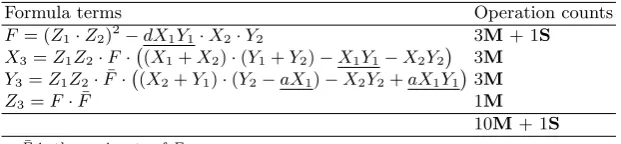
LetP = (X1, Y1, Z1) ∈Ea,d(Fp) be the base point andQ= (X2, Y2, Z2)∈ Ea,d(Fp) be a temporary derived point. Then,P+Qcan be improved by using our proposed steps. First, pre-compute the valuesX1·Y1, d·X1Y1, a·X1, and a·X1Y1. This pre-computation step costs 1M+ 1Md + 2Ma ≈2M. Then, the pre-computed values can be used with the proposedP+Qformula during scalar multiplication, as Table 2 shows. As a result,P+Qwith pre-computation saves 1Md + 1Ma ≈1M in comparison to P+Qwithout pre-computation. We say thatP+Qis mixedP+QwhenZ1= 1. The cost of mixedP+Qis 9M+ 1Md + 1Ma + 1S≈10.8M. It saves approximately 0.4M in comparison to mixed P+Qin Jacobian Weierstrass coordinates [28].
Table 2. Operation Counts for P +Q with pre-computation in Standard Twisted Edwards Coordinates overFp
Formula terms Operation counts
F = (Z1·Z2)2−dX1Y1·X2·Y2 3M+ 1S X3=Z1Z2·F· (X1+X2)·(Y1+Y2)−X1Y1−X2Y2
3M Y3=Z1Z2·F¯· (X2+Y1)·(Y2−aX1)−X2Y2+aX1Y13M
Z3=F·F¯ 1M
10M+ 1S ¯
F is the conjugate ofF.
Underlined terms are pre-computed.
2.3 A Proposed 2Q+P Formula
Theorem 1 Let P = (X1, Y1, Z1)∈Ea,d(Fp)andQ= (X2, Y2, Z2)∈Ea,d(Fp).
Then 2Q+P = (X3, Y3, Z3) in standard twisted Edwards coordinates is
repre-sented by
T =Y22+aX22
F =Z12T(T−2Z22) +dX1Y1 2X2Y2T¯ G= 2X2Y2(T −2Z22)
X3=F −TT X¯ 1Z1+Y1Z1G
Y3= ¯F −TT Y¯ 1Z1−aX1Z1G
Z3=FF¯
whereT¯ andF¯ are the conjugates ofT andF respectively.
Remark 1. 1. The cost of the proposed 2Q+P formula with pre-computation is 12M + 1Ma + 4S ≈ 15.2M, as Table 3 shows. It saves 1M + 1Md + 1S≈2.8M in comparison to a non-dedicated 2Q+P formula. The pre-computed values areZ2
1, X1·Y1, d·X1Y1, X1·Z1, Y1·Z1, X1Z1·Y1Z1, a·X1Z1, anda·X1Z1Y1Z1. This pre-computation step costs 4M + 1Md + 2Ma + 1S≈5.8M.
2. The cost of the proposed mixed 2Q+Pformula with pre-computation is 11M + 1Ma+ 4S≈14.2M. It saves 1M+ 1Md+ 1S≈2.8Min comparison to a non-dedicated mixed 2Q+P formula. It saves 3Sin comparison to 2Q+P in Jacobian Weierstrass (a= −3) coordinates, as Table 1 shows [29]. The cost of the proposed mixed 2Q+P formula without pre-computation is 12M + 1Md + 3Ma + 4S≈16.2M. It trades 1Swith 2Ma in comparison to a non-dedicated mixed 2Q+P formula. To the best of our knowledge, we are the first to propose a 2Q+P formula in twisted Edwards coordinates.
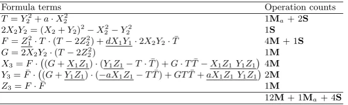
Table 3. Operation Counts for 2Q+P with Pre-computation in Standard Twisted Edwards Coordinates overFp
Formula terms Operation counts
T =Y2
2 +a·X22 1Ma + 2S
2X2Y2= (X2+Y2)2−X22−Y22 1S F =Z2
1·T·(T−2Z22) +dX1Y1·2X2Y2·T¯ 4M+ 1S
G= 2X2Y2·(T−2Z22) 1M
X3=F· (G+X1Z1)·(Y1Z1−T·T¯) +G·TT¯−X1Z1 Y1Z1
4M Y3= ¯F· (G+Y1Z1)·(−aX1Z1−TT¯) +GTT¯+aX1Z1 Y1Z12M
Z3=F·F¯ 1M
12M+ 1Ma + 4S ¯
T and ¯Fare the conjugate ofTandFrespectively. Underlined terms are pre-computed.
2.4 A Proposed 5P Formula
+ 3Ma + 9S ≈ 25.2M and the cost of 2P + 3P is 22M + 1Md + 3Ma + 8S≈29.4M. However, many studies show a dedicated 5P formula has a lower cost. Bernstein, Birkner, Lange, and Peters initially proposed two dedicated 5P formulas in standard Edwards coordinates with cost 17M + 7S≈22.6M and 14M + 11S≈ 22.8M [3]. Recently, Rao proposed a dedicated 5P formula in standard Edwards coordinates with cost 15M + 9S≈22.2M [37]. Li, Yu, and Wang proposed a 5P formula in standard Edwards coordinates with cost 12M + 12S≈21.6M[26]. We propose the most efficient 5P formula. See Theorem 2 for the proposed 5P formula and Appendix B for the proof.
Theorem 2 Let P = (X1, Y1, Z1)∈Ea,d(Fp). Then5P = (X5, Y5, Z5)in
stan-dard twisted Edwards coordinates is represented by
T =Y2 1 +aX12 A=TT¯+ 2Y2
1(T −2Z12) B =TT¯−2aX2
1(T−2Z12) C=−TT A¯ A¯+ 2Y2
1(T−2Z12)BB¯ D=TT B¯ B¯+ 2aX2
1(T−2Z12)AA¯ X5=X1CC¯
Y5=Y1DD¯ Z5=Z1CD
whereT ,¯ A,¯ B,¯ C,¯ andD¯ are the conjugates ofT, A, B, C, andD respectively.
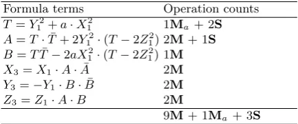
Remark 2. 1. The cost of the proposed 5P formula is 15M + 1Ma + 3S ≈ 17.4M, as Table 4 shows. It saves 4.2Mover Li et al.’s formula. Also, it saves approximately 2M in comparison to 5P in Jacobian Weierstrass (a=−3) coordinates, as Table 1 shows [17, 33, 30].
2. The proposed 5P formula needs only 2 temporary variables. This means that it can be performed using the same number of temporary variables as the 3P formula. See Appendix A for the cost of 3P in standard twisted Edwards coordinates and Appendix C for our proposed steps to perform the 3P and the 5P formulas with the fewest temporary variables.
3
MBNS Methods
3.1 Introduction
Table 4.Operation Counts for 5P in Standard Twisted Edwards Coordinates overFp
Formula terms Operation counts
T =Y12+a·X 2
1 1Ma+ 2S
A=T·T¯+ 2Y12·(T −2Z12) 2M+ 1S B=TT¯−2aX12·(T−2Z12) 1M C=−TT¯·A·A¯+ 2Y2
1(T−2Z12)·B·B¯4M D=TT¯·BB¯+ 2aX12(T−2Z12)·AA¯ 2M
X5=X1·C·C¯ 2M
Y5=Y1·D·D¯ 2M
Z5=Z1·C·D 2M
15M+ 1Ma + 3S ¯
T ,A,¯B,¯ C,¯ and ¯Dare the conjugates ofT , A, B, C,andDrespectively.
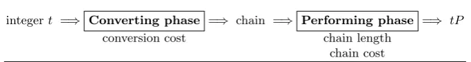
The converting phase The first phase of a method is to convert integert to a chain. A chain can be a single-base chain or a multi-base chain. We focus on three types of chains: a single-base chain with{2}-integers, a double-base chain with{2,3}-integers, and a multi-base chain with{2,3,5}-integers.
Definition 1 A positive integer t is represented in a multi-base chain with
{2,3,5}-integers in the form of
t= l X
i=1
si 2ai 3bi 5ci
where si ∈ {−1,+1} ,l is the chain length,a1 >a2 >· · · >al>0, b1 >b2>
· · ·>bl>0, andc1>c2>· · ·>cl>0.
Other studies proposed many methods that convert integert to single-base chains or multi-base chains. The binary and the NAF methods convert integert to a single-base chain with{2}-integers [20]. The greedy, the ternary/binary, the multi-base NAF, the tree-based, and the rDAG-based methods convert integer tto a multi-base chain [11, 33, 9, 27, 15, 39, 4]. These methods use different tech-niques to convert integert to a chain. Therefore, we use the converting cost to measure the converting phase of a method. We express the converting cost by the time complexity of converting integert to a chain. For example, the conversion cost of the binary method isO(log2t) and of the rDAG-based method is approx-imatelyO (log2t)2
. It is important to note that that the time complexity of the converting phase might not be an accurate evaluation. This is because the
integert =⇒ Converting phase =⇒ chain =⇒ Performing phase =⇒ tP
conversion cost chain length
chain cost
time complexity ignores the constant. The constant can affect the running time of the methods. It is hard to know the conversion cost of some methods, such as the greedy method. Therefore, we use our experimental results to determine the conversion cost of these methods.
The performing phase The second phase of a method is to perform a chain by executing a number of point addition (ADD), doubling (DBL), tripling (TPL), and quintupling (QPL) operations. The performing phase highly depends on a chain that is provided by the converting phase. We use the chain length and the chain cost to measure the performing phase. The chain length shows a broad indication of how good a chain is. It considers only the number of ADD to evaluate a chain. The chain cost shows an accurate indication of how good a chain is. It considers the number of ADD,DBL, TPL, andQPL to evaluate a chain.
Remark 3. Our theoretical studies and experimental results show that when integer t is represented by a multi-base chain, on average, we have a shorter length and a lower cost than a single-base chain.
The question is, why do the multi-base chains have a lower average cost than the single-base chain? In other words, why, when we replaceADD withDBL, TPL, or QPL, do we have lower average chain cost? We can explain that by the following reason. The cost of ADDis higher than the cost ofDBLin many coordinate systems. Even though the cost of ADD is lower than the cost of TPLandQPLin many coordinate systems, we still preferTPLandQPLover ADD because they are the least costly way to do three and five jumps. See Table 1 for the cost of ADD,DBL, TPL, andQPL in twisted Edwards and Jacobian coordinates.
An optimal chain There are no agreements among researchers on the definition of an optimal chain that represents integer t. However, we define an optimal chain as a chain that represents t with the lowest cost, as Definition 2 shows. The question is, do we have a method that generates an optimal chain? We know, as Experiment I shows, the greedy, ternary/binary, multi-base NAF, and tree-based methods do not produce an optimal chain. However, two methods were proposed by other studies to find an optimal chain: the enumeration approach and the rDAG-based method.
Definition 2 An optimal chain for integer tis a chain that representst, and it is the least costly in a particular coordinate system.
In the first study, Doche proposed the enumeration approach to find an opti-mal chain with respect to the length [14]. This is a type of brute force approach that takes exponential time to find an optimal chain. In the second study, Bern-stein, Chuengsatiansup, and Lange proposed the rDAG-based method to find an optimal chain with respect to the cost [4]. The conversion cost in the rDAG-based method is approximately O (log2t)2
. Even though the conversion cost of the rDAG-based method is much better than the conversion cost of the enumeration approach, the rDAG-based method seems impractical for applications that re-quire the converting phase to be on-the-fly, as Experiment II shows. We propose a solution to improve the rDAG-based method. We develop bucket methods to find a near optimal chain with the advantage of taking significantly less time than the rDAG-based method for an optimal chain. See Definition 3 for a near optimal chain definition and see the third result of Experiment II for a near optimal chain example.
3.2 Proposed Bucket Methods
DAG/bucket method The idea for this newly proposed method is to create buckets that are indexed by chain cost. A bucket contains nodes that are ordered by t. A node is represented in the form of (t,(s, a, b),(cost, seq),(prei, prej)) where :
t positive integer
(s, a, b) s2a3bwheres∈ {+1,0,−1}anda, b∈ {0,1} (cost, seq) costis chain cost
seqis a node sequence number in Bucket[i], andseq∈ {0, ..., bucket-size−1} (pre i, pre j)pre iis an index of the previous bucket
pre jis an index of the previous node in Bucket[pre i]
Algorithm 1 shows the steps of the DAG/bucket method. First, this method investigates nodes in a bucket with the lowest chain cost. Then, the method moves to the next bucket with the next lowest chain cost and investigates nodes. The method repeats the steps until it finds a node with t = 1. Finally, the method stops and returns the chain. Returning the chain is accomplished by get-chain, which traces (pre i, pre j) of nodes that are necessary for the chain. See Appendix D for an example of the DAG/bucket method.
An investigated node creates two or three nodes that are inserted into new buckets with a higher cost. This is because this method follows the DAG-based abstract idea, as Definition 4 shows. A node is inserted into a bucket accord-ing to its cost. The chain cost of nodes monotonically increases. This property guarantees that the method investigates all nodes and no node is skipped. Definition 4 The DAG-based abstract idea states that ift is odd, three options are investigated: (t−1)/2,(t+ 1)/2, and(t−s)/3. Iftis even, two options are investigated: t/2and(t−s)/3 wheres∈ {−1,0,+1}.
following way. The objective of the rDAG-based method is to find an optimal chain without paying much attention to the time it takes to reach it [4]. The objective of the DAG/bucket method is to provide flexibility to control the chain quality and the time to find the chain. The flexibility is obtained by bucket-size, a value which balances the chain quality and the time to find the chain.
Algorithm 1DAG/bucket Method Input:positive integert
Output:(s1, a1, b1), ...,(sl, al, bl) wherelis expansion length initializeBucket[bucket-max]
insert newnode(t,(0,0,0),(0,0),(0,0)) in Bucket[0]
fori←0tobucket-maxdo
if (Bucket[i] is empty)then continue for eachnodein Bucket[i]
if (node.t= 1)then returnget-chain(Bucket,i, node.seq)
for eachs∈ {+1,0,−1}
if ((node.t−s) (mod 2)≡0)then t←(node.t−s)/2
cost←node.cost+DBL+|s|ADD
insert newnode(t,(s,1,0),(cost, seq),(i, node.seq)) in Bucket[round(cost)]
removeany redundant nodes with respect tot
keepthe smallest nodes with respect totwithinbucket-size if ((node.t−s) (mod 3)≡0)then
t←(node.t−s)/3
cost←node.cost+TPL +|s|ADD
insert newnode(t,(s,0,1),(cost, seq),(i, node.seq)) in Bucket[round(cost)]
removeany redundant nodes with respect tot
keepthe smallest nodes with respect totwithinbucket-size
Tree/bucket method The idea of the tree/bucket method is to create buckets that are indexed by chain length. A bucket contains nodes that are ordered by t. A node is represented in the form of (t,(s, a, b),(seq, pre)) where:
t positive integer
(s, a, b) s2a3bwheres∈ {+1,0,−1}anda, b≥0
(seq, pre)seqis a node sequence number in Bucket[i], andseq∈ {0, ..., bucket-size−1}
preis an index of the previous node in Bucket[i−1]
which tracespreof nodes that are necessary for the chain. See Appendix D for an example of the tree/bucket method.
An investigated node always creates two new nodes that are inserted into the next bucket. This is because the tree/bucket method follows the tree-based abstract idea, as Definition 5 shows. A node is inserted into a bucket according to its length. The chain length of nodes monotonically increases. This property guarantees that the method investigates all nodes and no node is skipped.
Definition 5 The tree-based abstract idea states that if t is coprime with 6, then two options are investigated: (t+ 1)/(2a3b) and (t−1)/(2a3b) where a, b
are 2-adic and3-adic valuations of(t+ 1) or(t−1).
The similarity between the DAG/bucket and tree/bucket methods is that they both use bucket-size to control the chain quality and the time to find a chain. The main difference between them is that the tree/bucket method utilizes the tree-based abstract idea, and the DAG/bucket method utilizes the DAG-based abstract idea. As a result, the DAG/bucket method generates a higher chain quality than the tree/bucket method, and the tree/bucket method generates a chain faster than the DAG/bucket method, as Experiment II shows.
Algorithm 2Tree/bucket Method Input:positive integert
Output:(s1, a1, b1), ...,(sl, al, bl) wherelis chain length initializeBucket[bucket-max]
t←t/(2a3b) wherea, bare 2-adic and 3-adic valuations oft insert newnode(t,(0, a, b),(0,0)) in Bucket[1]
fori←1tobucket-maxdo
if (Bucket[i] is empty)then continue for eachnodein Bucket[i]
if (node.t= 1)then returnget-chain(Bucket,i, node.seq) for eachs∈ {+1,−1}
t←(node.t−s)/(2a3b) wherea, bare 2-adic and 3-adic valuations of (node.t−s) insert newnode(t,(s, a, b),(seq, node.seq)) in Bucket[i+ 1]
removeany redundant nodes with respect tot
keepthe smallest nodes with respect totwithinbucket-size
The second factor that impacts the chain quality in the bucket methods is bucket-max. Bucket-max determines the number of buckets that are needed at maximum to find a chain. Experimentally, we found that when buckets are indexed by chain cost, bucket-max does not exceed the average chain cost of the NAF method. When buckets are indexed by chain length, bucket-max does not exceed the average chain length of the NAF method. This is with the assumption that the DAG/bucket method rounds the chain cost to the nearest integer. As a result, the average chain length and the average chain cost of the NAF method can estimate the value of bucket-max in the bucket methods. The average chain length of the NAF method is approximately (log2t)/3. The average chain cost of the NAF method is approximatelylog2t(1/3ADD +DBL).
4
Experimental Results
In this section, we show the results of two experiments. Experiment I compares the multi-base methods with the single-base methods. Experiment II compares the DAG/bucket method with the tree/bucket method. We incorporated our ef-ficient formulasP+Q,2Q+P and 5P in these MBNS methods. We conducted these experiments in standard twisted Edwards coordinates over prime fields. We used three types of measurements to compare the methods: the average chain length, the average chain cost, and the average running time.
The advantage of the chain length and the chain cost measurements is that they give the same results if we test the methods in different devices. This is because the chain length is affected by the integer bit size and the method. The chain cost is effected by the integer bit size, the method, the coordinate system, and the S/M ratio assumption. For the chain cost, we ignored addi-tion/subtraction operations since they are cheap operations. We assumed 1S= 0.8M over prime fields. We did not use inversion operations since we worked in projective coordinates.
The advantage of the running time measurement is that it evaluates all the implementation aspects of the methods. It takes into consideration, unlike other measurements, the time to convert integertto a chain. The disadvantage of the running time measurement is that it gives different results if we test the methods in different devices. This is because the running time is affected directly by var-ious factors such as the CPU specification, the number of temporary variables, and the finite field arithmetic library (e.g., GMP, MIRCAL) [18, 31].
4.1 Experiment I
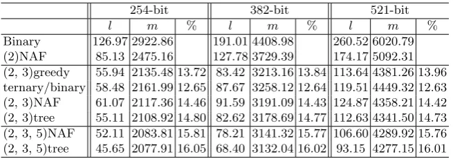
The goal for Experiment I was to compare the single-base methods with the multi-base methods. We wanted to measure the obtained improvement if the multi-base methods were used over the single-base methods. For the single-base methods, we implemented the binary and the NAF methods [20]. For the multi-base methods, we implemented the greedy, the ternary/binary, the multi-multi-base NAF, and the tree-based methods [11] [9, 27, 15]. We assumed bound-size = 1 in the tree-based method because we did not consider the pre-computation option in Experiment I. However, we considered the pre-computation option in the converting phase in Experiment II. We present the results of Experiment I in Table 5 and Table 6. It shows the comparison results of the single-base and the multi-base methods with respect to the average chain length (l), the average chain cost (m), and the average running time (t).
Table 5.Theoretical Comparison Between Single-base and Multi-base Methods
254-bit 382-bit 521-bit
l m % l m % l m %
Binary 126.97 2922.86 191.01 4408.98 260.52 6020.79
(2)NAF 85.13 2475.16 127.78 3729.39 174.17 5092.31
(2, 3)greedy 55.94 2135.48 13.72 83.42 3213.16 13.84 113.64 4381.26 13.96 ternary/binary 58.48 2161.99 12.65 87.67 3258.12 12.64 119.51 4449.32 12.63 (2, 3)NAF 61.07 2117.36 14.46 91.59 3191.09 14.43 124.87 4358.21 14.42 (2, 3)tree 55.11 2108.92 14.80 82.62 3178.69 14.77 112.63 4341.50 14.73 (2, 3, 5)NAF 52.11 2083.81 15.81 78.21 3141.32 15.77 106.60 4289.92 15.76 (2, 3, 5)tree 45.65 2077.91 16.05 68.40 3132.04 16.02 93.15 4277.15 16.01
l:The average chain length. m:The average chain cost.
%:The improvement percentage with respect tomin comparison to (2)NAF.
Results of Experiment I We obtained three main results from Experiment I. First, with respect to m, all the investigated multi-base methods performed better than the single-base methods. We saw that the multi-base methods gave approximately 12% to 16% improvement in comparison to the single-base NAF method. With respect tot, they gave approximately 12% to 18% improvement, except for the greedy method (addressed below). The tree-based method with
{2,3,5}-integers succeeded to give the highest percentage of improvement in comparison to other methods.
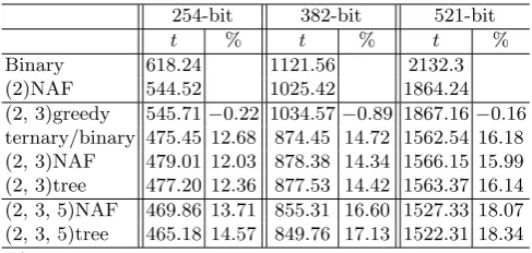
Table 6.Running Time Comparison Between Single-base and Multi-base Methods
254-bit 382-bit 521-bit
t % t % t %
Binary 618.24 1121.56 2132.3
(2)NAF 544.52 1025.42 1864.24
(2, 3)greedy 545.71−0.22 1034.57−0.89 1867.16−0.16 ternary/binary 475.45 12.68 874.45 14.72 1562.54 16.18 (2, 3)NAF 479.01 12.03 878.38 14.34 1566.15 15.99 (2, 3)tree 477.20 12.36 877.53 14.42 1563.37 16.14 (2, 3, 5)NAF 469.86 13.71 855.31 16.60 1527.33 18.07 (2, 3, 5)tree 465.18 14.57 849.76 17.13 1522.31 18.34
t:The average running time inµs.
%:The improvement percentage in comparison to (2)NAF.
to double-base methods was higher than the improvement from double-base to triple-base methods. As a result, we conclude that 7Pand 11P dedicated formu-las seem impractical to use with the multi-base methods since they only achieve a minor improvement.
Lastly, we found that the greedy method with{2,3}-integers is impractical for implementation for two reasons. The first reason is that it requires extra set-up time to find the best upper bound (amax, bmax). We found that the upper bounds (140,73), (210,109), and (290,146) are approximately the best value for 254-bit, 382-bit, and 521-bit integers respectively. In contrast, other multi-base methods do not require extra set-up time to find the best upper bound.
The second reason it is impractical is the converting time. We did not have an efficient way to find the best approximation for integertin terms of a{2,3} -integer. However, we tried the best available solutions. We used the line search al-gorithm [39, 7]. Another option is to use a look-up table [16]. However, a look-up table requires an offline pre-computation and extra memory space. In contrast, the converting times in other multi-base methods are more efficient and do not require offline pre-computations. This is because they use a dynamic approach to convert integer tto a multi-base chain.
4.2 Experiment II
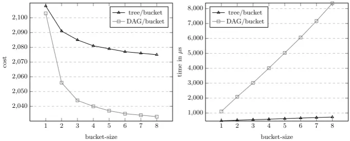
The goal of Experiment II was to compare the tree/bucket and the DAG/bucket methods. We wanted to measure the bucket-size impact of the bucket methods on the chain cost and the time to find the chain. We implemented the DAG/bucket and tree/bucket methods with {2,3}-integers by using Algorithm 1 and Algo-rithm 2 respectively. We focused on 254-bit integers. We present the results of Experiment II in Figure 2. It shows the bucket-size impact of bucket methods on the chain cost and the time to find the chain.
1 2 3 4 5 6 7 8 2,040
2,050 2,060 2,070 2,080 2,090 2,100
bucket-size
cost
tree/bucket DAG/bucket
1 2 3 4 5 6 7 8 1,000
2,000 3,000 4,000 5,000 6,000 7,000 8,000
bucket-size
time
in
µ
s
tree/bucket DAG/bucket
Fig. 2.Experimental Comparison Between Tree/bucket and DAG/bucket Methods
the time to find the chain. We noted that when the bucket-size increases, the chain cost gradually decreases and the time to find a chain gradually increases. The largest improvement of the chain cost in the bucket methods was when size = 2. The improvement of the chain cost became minor when bucket-size>4. As a result, we concluded that the bucket methods seem more practical when the bucket-size is selected from 2 to 4.
Second, the DAG/bucket method produces a lower chain cost than the tree/bucket method. However, the DAG/bucket method also requires more time to find a chain. This is due to the ways these methods generate new nodes, as explained in Section 3. We also saw that the tree/bucket method with bucket-size = ∞
cannot produce a lower chain cost than the DAG/bucket method with bucket-size >1. This implies that the tree-based method with unbound-size does not produce an optimal chain nor a near optimal chain, as Table 7 shows.
Table 7.Experimental Comparison Between Optimal and Near Optimal Chains
254-bit
l m t
(2, 3)tree/bucketsize=∞ 51.01 2070.73
(2, 3)DAG/bucketsize=4 51.54 2040.01 4008.17
(2, 3)rDAG-based 49.61 2035.56 14941.53
l:The average chain length. m:The average chain cost. t:The average running time inµs.
method when bucket-size = 4 is 2040.01M. Therefore, the difference between them is less than DBLcost. We also noted that the near optimal chain of the DAG/bucket method sped up the performance 73.17% in comparison to the optimal chain. This is because the time to reach an optimal chain in the rDAG-based method is 14941.53µs and the time to reach a near optimal chain in the DAG/bucket method is 4008.17µs, as Table 7 shows.
5
Conclusion
In this paper, we consider the efficiency problem of scalar multiplication for elliptic curves over finite fields with a twofold focus. Our first focus was to derive several efficiently computable formulas for the class of twisted Edwards curves over prime fields. We proposed 2Q+P and 5P formulas in standard projective coordinate systems. To the best of our knowledge, the 2Q+P formula given in this paper is the first dedicated formula for twisted Edwards curves. It saves about 2.8 field multiplications, compared to a non-dedicated formula. Our 5P formula improves on the best one in the literature [26] by about 4.2 field multiplications. Our 2Q+P saves 3 field squarings and our 5P saves about 2 field multiplications, compared to 2Q+P and 5P in Jacobian Weierstrass (a=−3) coordinates. In addition, using the pre-computation concept, we were able to compute P+Qwith one less field multiplication.
Our second focus dealt with the efficiency of generating MBNS chains. We formulated bucket methods for the DAG-based and the tree-based abstract ideas. These proposed bucket methods systematically balance the chain quality and the time to find the chain. We proposed finding a near optimal chain that relaxes the requirement of a chain being optimal. This is because finding a near optimal chain is more efficient than finding an optimal chain. We also demonstrated that the tree-based method does not produce an optimal chain nor a near optimal chain.
References
1. Al Musa, S., Xu, G.: Fast scalar multiplication for elliptic curves over binary field-s by efficiently computable formulafield-s. In: Patra, A., Smart, N. (edfield-s.) Proc. IN-DOCRYPT 20017. pp. 206–226. LNCS, Springer, Cham (2017)
2. Bernstein, D., Birkner, P., Joye, M., Lange, T., Peters, C.: Twisted edwards curves. In: Vaudenay, S. (ed.) Proc. AFRICACRYPT 2008. pp. 389–405. LNCS, Springer, Heidelberg (2008)
3. Bernstein, D., Birkner, P., Lange, T., Peters, C.: Optimizing double-base elliptic curve single-scalar multiplication. In: Srinathan, K., Rangan, C., Yung, M. (eds.) Proc. INDOCRYPT 2007 . pp. 167–182. LNCS, Springer, Heidelberg (2007) 4. Bernstein, D., Chuengsatiansup, C., Lange, T.: Double-base scalar multiplication
revisited. Cryptology ePrint Archive, Report 2017/037 (2017), https://eprint. iacr.org/2017/037
5. Bernstein, D., Lange, T.: Inverted edwards coordinates. In: Boztas, S., Lu, H. (eds.) Proc. AAECC 2007. pp. 20–27. LNCS, Springer, Heidelberg (2007)
6. Bernstein, D., Lange, T.: Faster addition and doubling on elliptic curves. Cryptolo-gy ePrint Archive, Report 2007/286 (2007),https://eprint.iacr.org/2007/286
7. Berthe, V., Imbert, L.: On converting numbers to the double-base number system. Adv. Signal Pro. Algo. Archit. Implement. XIV.5559, 7078 (2004)
8. Brown, M., Hankerson, D., Lopez, J., Menezes, A.: Software implementation of the nist elliptic curves over prime fields. In: Naccache, D. (ed.) Proc. CT-RSA 2001. pp. 250–265. LNCS, Springer, Heidelberg (2001)
9. Ciet, M., Joye, M., Lauter, K., Montgomery, P.: Trading inversions for multipli-cations in elliptic curve cryptography. Designs, Codes and Cryptography 39(2), 189–206 (2006)
10. Crosby, M., Nachiappan, Pattanayak, P., Verma, S., Kalyanaraman, V.: Blockchain technology: Beyond bitcoin (2016), http://scet.berkeley.edu/wp-content/ uploads/AIR-2016-Blockchain.pdf
11. Dimitrov, V., Imbert, L., Mishra, P.: Efficient and secure elliptic curve point mul-tiplication using double-base chains. In: Roy, B. (ed.) Proc. ASIACRYPT 2005. pp. 59–78. LNCS, Springer, Heidelberg (2005)
12. Dimitrov, V., Imbert, L., Mishra, P.: The double-base number system and its application to elliptic curve cryptography. Mathematics of Computation77(262), 1075–1104 (2008)
13. Dimitrov, V., Jullien, G., Miller, W.: An algorithm for modular exponentiation. Information Processing Letters66, 155–159 (1998)
14. Doche, C.: On the enumeration of double-base chains with applications to elliptic curve cryptography. In: Sarkar, P., Iwata, T. (eds.) Proc. ASIACRYPT 2014. pp. 297–316. LNCS, Springer, Heidelberg (2014)
15. Doche, C., Habsieger, L.: A tree-based approach for computing double-base chains. In: Mu, Y., Susilo, W., Seberry, J. (eds.) Proc. ACISP 2008. pp. 433–446. LNCS, Springer, Heidelberg (2008)
16. Doche, C., Imbert, L.: Extended double-base number system with applications to elliptic curve cryptography. In: Barua, R., Lange, T. (eds.) Proc. INDOCRYPT 2006. pp. 335–348. LNCS, Springer, Heidelberg (2006)
17. Giorgi, P., Imbert, L., Izard, T.: Optimizing elliptic curve scalar multiplication for small scalars. Mathematics for Signal and Information Processing7444(2009) 18. Granlund, T., et al.: Gnu multiple precision arithmetic library, http://www.
19. Hankerson, D., Lopez, J., Menezes, A.: Software implementation of elliptic curve cryptography over binary fields. In: Koc, C., Paar, C. (eds.) Proc. CHES 2000. pp. 1–24. LNCS, Springer, Heidelberg (2000)
20. Hankerson, D., Menezes, A., Vanstone, S.: Guide to elliptic curve cryptography. Springer-Verlag (2004)
21. He, D., Zeadally, S.: An analysis of rfid authentication schemes for internet of things in healthcare environment using elliptic curve cryptography. IEEE Internet of Things Journal2, 72–83 (2014)
22. Koblitz, N.: Elliptic curve cryptosystems. Math. of Computation48(177), 203–209 (1987)
23. Kohel, D.: Twisted u4-normal form for elliptic curve. Cryptology ePrint Archive, Report 2017/121 (2017),https://eprint.iacr.org/2017/121
24. Lange, T.: A note on lopez-dahab coordinates. Cryptology ePrint Archive, Report 2004/323 (2004),https://eprint.iacr.org/2004/323
25. Lenstra, A., Verheul, E.: Iselecting cryptographic key sizes. Journal of Cryptology
14, 255–293 (2001)
26. Li, W., Yu, W., Wang, K.: Improved tripling on elliptic curves. In: Lin, D., Wang, X., Yung, M. (eds.) Proc. Inscrypt 2015. pp. 193–205. LNCS, Springer, Cham (2016)
27. Longa, P., Gebotys, C.: Fast multibase methods and other several optimizations for elliptic curve scalar multiplication. In: Jarecki, S., Tsudik, G. (eds.) Proc. PKC 2009. pp. 443–462. LNCS, Springer, Heidelberg (2009)
28. Longa, P., Miri, A.: Fast and flexible elliptic curve point arithmetic over prime fields. IEEE Transactions on Computers57, 289–302 (2008)
29. Longa, P., Miri, A.: New composite operations and precomputation scheme for elliptic curve cryptosystems over prime fields. In: Cramer, R. (ed.) Proc. PKC 2008. pp. 229–247. LNCS, Springer, Heidelberg (2008)
30. Longa, P., Miri, A.: New multibase non-adjacent form scalar multiplication and its application to elliptic curve cryptosystems (extended version). Cryptology ePrint Archive, Report 2008/052 (2008),https://eprint.iacr.org/2008/052
31. Matula, D., Kornerup, P.: Multiprecision integer and rational arithmetic c library,
http://www.miracl.com
32. Miller, V.: Use of elliptic curves in cryptography. In: Williams, H. (ed.) Proc. CRYPTO 1985. pp. 417–426. LNCS, Springer, Heidelberg (1986)
33. Mishra, P., Dimitrov, V.: Efficient quintuple formulas for elliptic curves and effi-cient scalar multiplication using multibase number representation. In: Garay, J., Lenstra, A., Mambo, M., Peralta, R. (eds.) Proc. ISC 2007 . pp. 390–406. LNCS, Springer, Heidelberg (2007)
34. Nakamoto, S.: Bitcoin: A peer-to-peer electronic cash system (2011), https:// bitcoin.org/bitcoin.pdf
35. Oliveira, T., Lopez, J., Aranha, D., Rodriguez-Henriquez, F.: Two is the fastest prime: lambda coordinates for binary elliptic curves. Journal of Cryptographic Engineering4(1), 3–17 (2014)
36. Rescorla, E.: Rfc8446: The Transport Layer Security (TLS) Protocol Version 1.3 (2018)
38. Yu, W., Kim, K., Jo, M.: New fast algorithms for elliptic curve arithmetic in affine coordinates. In: Tanaka, K., Suga, Y. (eds.) Proc. IWSEC 2015. pp. 56–64. Springer, Cham (2015)
6
Appendix A: Formulas
This appendix shows the operation counts for P +Q, 2P, and 3P formulas represented in standard twisted Edwards coordinates. These formulas can be found in [2, 4]. However, we use different notations to present these formulas because we want to unify the notations for the complete setP+Q, 2P, 3P, and 5P. Also, it is necessary to present these formulas here because the proofs of the new 5P, and 2Q+P formulas depend on these formulas.
Table 8.Operation Counts forP+Qin Standard Twisted Edwards Coordinates
Formula terms Operation counts
F = (Z1·Z2)2−d·X1·X2·Y1·Y2 4M+1Md+1S X3=Z1Z2·F· (X1+Y1)·(X2+Y2)−X1X2−Y1Y23M
Y3=Z1Z2·F¯·(Y1Y2−a·X1X2) 2M+1Ma
Z3=F·F¯ 1M
10M+1Md+1Ma+1S ¯
F is the conjugate ofF.
Table 9.Operation Counts for 2P in Standard Twisted Edwards Coordinates
Formula terms Operation counts
T =Y12+a·X 2
1 1Ma+ 2S
X2= (X1+Y1)2−X12−Y12
·(T−2Z12) 1M+ 2S
Y2=−T·T¯ 1M
Z2=T·(T−2Z12) 1M
3M+ 1Ma+ 4S ¯
T is the conjugate ofT.
Table 10.Operation Counts for 3P in Standard Twisted Edwards Coordinates
Formula terms Operation counts
T =Y12+a·X12 1Ma + 2S A=T·T¯+ 2Y2
1 ·(T −2Z12) 2M+ 1S
B=TT¯−2aX12·(T−2Z12) 1M X3=X1·A·A¯ 2M Y3=−Y1·B·B¯ 2M Z3=Z1·A·B 2M
9M+ 1Ma + 3S ¯
7
Appendix B: Proofs
7.1 Proof of Theorem 1
Proof. We shall prove Theorem 1 by the fact
(X2Q+P, Y2Q+P, Z2Q+P) = (X2Q, Y2Q, Z2Q) + (XP, YP, ZP).
From theP+Qformula in Table 8, We have
F = (ZPZ2Q)2−dXPYPX2QY2Q.
We substituteX2Q, Y2Q, Z2Q with their equivalent terms in Table 9. We have
T =YQ2+aXQ2. F = ZPT(T−2ZQ2)
2
+dXPYP2XQYQ(T−2ZQ2)TT¯ =T(T−2ZQ2) ZP2T(T−2ZQ2) +dXPYP2XQYQT¯
.
From theP+Qformula, we have
X2Q+P =ZPZ2QF(XPY2Q+YPX2Q). Y2Q+P =ZPZ2QF¯(YPY2Q−aXPX2Q). Z2Q+P =FF .¯
We cancelZ2Qby the factsx2Q+P =X2Q+P/Z2Q+Pandy2Q+P =Y2Q+P/Z2Q+P. We have
F =ZP2T(T−2ZQ2) +dXPYP2XQYQT .¯ X2Q+P =ZPF(XPY2Q+YPX2Q).
Y2Q+P =ZPF¯(YPY2Q−aXPX2Q). Z2Q+P =FF .¯
ForX2Q+P, we substituteX2Q, Y2Q with their equivalent terms. We have
G= 2XQYQ(T−2ZQ2). X2Q+P =ZPF XP(−TT) +¯ YPG
.
=F −TT X¯ PZP +YPZPG
.
=F (G+XPZP)(YPZP−TT¯) +GTT¯−XPYPZP2
.
ForY2Q+P, we substituteX2Q, Y2Q with their equivalent terms. We have
Y2Q+P =ZPF Y¯ P(−TT¯)−aXPG
.
= ¯F −TT Y¯ PZP−aXPZPG.
=F (G+YPZP)(−aXPZP−TT¯) +GTT¯+aXPYPZP2
7.2 Proof of Theorem 2
Proof. We shall prove Theorem 2 by the fact 5P = 2P + 3P. From the P+Q formula shown in Table 8, we have
F = (Z2·Z3)2−dX2X3Y2Y3.
We substitute X2, Y2, Z2, X3, Y3, Z3 with their equivalent terms in Table 9 and Table 10. We have
F = T(T−2Z12)Z1AB 2
−2dX12Y12(T−2Z12)AAT¯ T B¯ B.¯ From the curve equationdX12Y12=Z12(T−Z12), we have
F= T(T−2Z12)Z1AB 2
−2Z12(T−Z12)(T−2Z12)AAT¯ T B¯ B¯ =T(T−2Z12)Z12AB T(T−2Z12)AB−2(T−Z12) ¯AT¯B¯
.
From the P+Q formula, we have
X5=Z2Z3F(X2Y3+Y2X3). Y5=Z2Z3F(Y¯ 2Y3−aX2X3). Z5=FF .¯
We cancelZ2Z3 by the factsx5=XZ55 andy5= YZ55. We have F =T(T−2Z12)AB−2(T−Z12) ¯AT¯B.¯ X5=F(X2Y3+Y2X3).
Y5= ¯F(Y2Y3−aX3X2). Z5=Z1FF .¯
ForX5, we substituteX2, X3, Y2, X3 with their equivalent terms. We have X5=F −2X1Y1(T−2Z12)Y1BB¯−TT X¯ 1AA¯
=X1F −TT A¯ A¯−2Y12(T−2Z 2 1)BB¯
.
Let ¯C = −TT X¯ 1AA¯−2X1Y12(T −2Z12)BB. Then¯ C = F where ¯C is the conjugate ofC. Thus, we have
X5=X1CC.¯
ForY5, we also substituteX2, X3, Y2, Y3with their equivalent terms. We have Y5= ¯F TT Y¯ 1BB¯−aX1AA2X¯ 1Y1(T−2Z12)
=Y1F T¯ T B¯ B¯−2aX12AA(T¯ −2Z 2 1)
.
Let ¯D =TT B¯ B¯−2aX12AA(T¯ −2Z12). ThenD = ¯F where ¯D is the conjugate ofD. Thus, we have
Y5=Y1DD.¯
8
Appendix C: Algorithms
Algorithm 3 and Algorithm 4 show that point tripling (TPL), and point quin-tupling (QPL) in standard twisted Edwards coordinates need only 2 temporary variables. See Table 10 and Table 4 for the 3P and the 5P formulas.
Algorithm 3Point Tripling Input:P = (X, Y, Z) Output:3P = (X3, Y3, Z3) X3=Y2
Y3=X2 Y3=a·X3 Z3=X3+Y3 T1=X3−Y3 T1=T1·Z3 T2=Z2 T2=T2+T2 T2=Z3−T2 X3=X3+X3 X3=X3·T2 Y3=Y3+Y3 Y3=Y3·T2 Z3=T1+X3 X3=T1−X3 X3=X3·Z3 T2=T1−Y3 Y3=T1+Y3 Y3=Y3·T2 Z3=Z3·T2 Z3=Z·Z3 X3=X·X3 Y3=Y ·Y3 Y3=−Y3
return:(X3, Y3, Z3)
Algorithm 4Point Quintupling Input:P = (X, Y, Z)
Output:5P = (X5, Y5, Z5) Z5=Y2
Y5=X2 Y5=a·Y5 X5=Z5+Y5 T1=Z2 T1=T1+T1 T1=X5−T1 Z5=Z5+Z5 Y5=Y5+Y5 Z5=Z5·T1 T1=Y5·T1 Y5=X5−Y5 Y5=Y5·X5 X5=Y5+Z5 T2=Y5−Z5 X5=X5·T2 T2=Y5−T1 Y5=Y5+T1 Y5=T2·Y5 T2=T2+T1 T1=T1·X5 Z5=Z5·Y5 X5=T2·X5 X5=−X5 Y5=T2·Y5 T2=X5+Z5 X5=X5−Z5 X5=T2·X5 X5=X·X5 Z5=Y5+T1 Y5=Y5−T1 Y5=Z5·Y5 Y5=Y ·Y5 Z5=T2·Z5 Z5=Z·Z5
9
Appendix D: Examples
9.1 DAG/bucket method
We want to find a chain fort= 13 using the DAG/bucket method with{2,3} -integers. Assume the cost of ADD = 2, DBL = 1, TPL = 2. Algorithm 1 creates the following buckets:
cost nodes
0 (13,(0,0,0),(0,0),(0,0))
3 (6,(1,1,0),(3,0),(0,0)), (7,(−1,1,0),(3,1),(0,0)) 4 (3,(0,1,0),(4,0),(3,0)), (4,(1,0,1),(4,1),(0,0)) 5 (2,(0,0,1),(5,0),(3,0))
6 (1,(0,0,1),(6,0),(4,0)), (3,(1,1,0),(6,1),(3,1)), (4,(−1,1,0),(6,2),(3,1)) 7 (1,(1,1,0),(7,0),(4,0)), (2,(1,0,1),(7,1),(3,1))
8 (1,(1,0,1),(8,0),(4,1)) 9 (1,(−1,0,1),(9,0),(5,0))
Then, getting the chain steps can be accomplished by the following Horner’s rule manner:
(1,(0,0,1),(6,0),(4,0)) =⇒ chain = 3 (3,(0,1,0),(4,0),(3,0)) =⇒ chain = (3)2 (6,(1,1,0),(3,0),(0,0)) =⇒ chain = ((3)2)2 + 1. Thus, chain = 223 + 1 = 13.
9.2 Tree/bucket method
We want to find a chain for t = 29 using the tree/bucket method with{2,3} -integers. Algorithm 2 creates the following buckets:
length nodes
1 (29,(0,0,0),(0,0))
2 (5,(−1,1,1),(0,1)), (7,(1,2,0),(1,1)) 3 (1,(1,2,0),(0,2))
Getting the chain steps can be accomplished by the following Horner’s rule manner:
(1,(1,2,0),(0,2)) =⇒ chain = 22+ 1