DOI: 10.1534/genetics.104.031484
A Unified Statistical Model for Functional Mapping of Environment-Dependent
Genetic Expression and Genotype
⫻
Environment Interactions
for Ontogenetic Development
Wei Zhao,* Jun Zhu,
†Maria Gallo-Meagher
‡and Rongling Wu*
,1*Department of Statistics and‡Agronomy Department, University of Florida, Gainesville, Florida 32611 and†Department of Agronomy, Zhejiang University, Hangzhou, Zhejiang 310029, People’s Republic of China
Manuscript received May 21, 2004 Accepted for publication August 10, 2004
ABSTRACT
The effects of quantitative trait loci (QTL) on phenotypic development may depend on the environment (QTL⫻environment interaction), other QTL (genetic epistasis), or both. In this article, we present a new statistical model for characterizing specific QTL that display environment-dependent genetic expressions and genotype⫻environment interactions for developmental trajectories. Our model was derived within the maximum-likelihood-based mixture model framework, incorporated by biologically meaningful growth equations and environment-dependent genetic effects of QTL, and implemented with the EM algorithm. With this model, we can characterize the dynamic patterns of genetic effects of QTL governing growth curves and estimate the global effect of the underlying QTL during the course of growth and development. In a real example with rice, our model has successfully detected several QTL that produce differences in their genetic expression between two contrasting environments. These detected QTL cause significant genotype⫻environment interactions for some fundamental aspects of growth trajectories. The model provides the basis for deciphering the genetic architecture of trait expression adjusted to different biotic and abiotic environments and genetic relationships for growth rates and the timing of life-history events for any organism.
A
number of statistical methods have been developed means of different QTL genotypes at different time points,but rather fit these means using growth curves as a to map quantitative trait loci (QTL) affecting
com-plex traits in well-structured pedigrees (Lander and function of time. Thus, the estimation of QTL effects on
growth is equivalent to the estimation of model parameters
Botstein 1989; Jansen 2000) or natural populations
(Wuet al.2002a). These methods have been instrumen- describing the shape of growth curves. These models,
calledfunctional mapping, have successfully detected
dy-tal in the identification of QTL responsible for various
quantitative traits of agricultural, biological, or biomedi- namic QTL that affect developmental changes during
ontogenetic growth in a long-lived forest tree (Wuet al.
cal value (Wuet al. 2000;Mackay 2001;Zimdahlet al.
2002). However, the derivations of these statistical meth- 2003) and the animal model system—mouse (Zhaoet
al.2004).
ods that were based on a simplified assumption that
there is a direct relationship between the genotype and Current functional mapping models that have
exam-ined the effects of individual QTL on growth trajectories phenotype did not consider sequential developmental
pathways that form the phenotype. It is likely, therefore, have focused on a particular phenotype measured at a
finite set of time points in a single environment (Maet
that these methods lead to biased estimation of QTL
positions and effects and have limited power to detect al.2002;Wuet al.2002b). Other studies have examined
genotype⫻ environment interactions involving
multi-QTL involved.
More recently, a host of new statistical models have ple environments (Piepho2000), but have focused on
a single measurement of a phenotype and hence cannot been proposed to map a complex trait by taking into
provide a comprehensive picture of how a QTL affects
account its underlying developmental changes (Maet al.
the dynamic process of growth under a range of
environ-2002;Wuet al.2002b, 2004a,b). These models integrate
mental conditions.Wuet al.(2004a) proposed a model
universal growth laws derived from fundamental
biologi-for characterizing the effects of epistatic QTL on growth cal principles and described by mathematical models
trajectories but did not incorporate environmental in-into a QTL mapping framework through statistics as a
fluences into the model. bridge. They do not directly estimate the expected
A great wealth of evidence suggests that different ex-pressions of the same genotype across environmental
contexts, referred to as phenotypic plasticity (Wu1998),
1Corresponding author:Department of Statistics, 533 McCarty Hall C,
University of Florida, Gainesville, FL 32611. E-mail: [email protected] are controlled by specific QTL (Mackay2001) through
two different but not exclusive genetic mechanisms, al- ally cease. von Bertalanffy also noted that the metabolic rate of an animal [in fact, any organism, as observed by
lelic sensitivity and gene regulatory control (Wu1998;
Vieiraet al.2000). Yanet al.(1998) identified several succeeding researchers (Westet al.2001)], scales as the
kth power of its weight (Niklas1994;Westet al.1997)
QTL on the rice genome that display significant
geno-type⫻environment interaction effects on plant height but the catabolic rate is proportional to the weight itself.
Therefore, the growth rate,i.e., the difference between
measured at multiple time points of development,
al-though their results were derived from interval mapping these two rates, becomes
of single phenotypes. In her seminal review, Mackay
(2001) claimed the existence of environment-specific dg(t)
dt ⫽ g
k(t)⫺ g(t) , (1)
QTL that direct organismic development toward the
best utilization of resources in heterogeneous environ- where g(t) represents the growth at timet andand
ments. are the constants of metabolism and catabolism,
re-In this article, we extend our previous functional map- spectively. For small values ofk, integration of Equation
ping model to map QTL that display genotype⫻envi- 1 leads to the growth equation,
ronment interactions for developmental trajectories. Al-though this extended model is similar to the previous
g(t)⫽
冦
⫺
冤
⫺ g10⫺k
冥
e⫺(1⫺k)t冧
1/(1⫺k), (2)
epistatic model (Wuet al.2004a) in modeling the mean
vector for time-dependent genotypic values, these two
whereg0is the growth att⫽0. This growth function is
models are methodologically different in modeling the
sigmoidal (S-shaped), approaching asymptotically the
(co)variance matrix for longitudinal measurements of
value (/)1/(1⫺k)ast → ∞. Such anS-shaped pattern
growth. The epistatic model needs to model only the
of growth includes an exponential growth stage, an as-structure of one (co)variance matrix, whereas the
geno-ymptotic growth stage, and the point of inflection at
type⫻environment interaction model needs to model
which these two stages are connected (Westet al.1999).
multiple (co)variance matrices each corresponding to
At the point of inflection, an organism displays maxi-an environment as well as to model the covarimaxi-ances
mum growth per unit time. After the substitutions, between different environments.
Our extended model for characterizing genotype⫻
a1⫺k⫽
environment interactions is constructed within the max-imum-likelihood-based mixture model framework and unifies the genetic effects of QTL expressed in different
b⫽ ⫾
冢
⫺g10⫺k
冣
ak⫺1environments through biological principles and statisti-cal models. We incorporate the EM algorithm to solve
r⫽ (1⫺k), the mixture model and provide estimates of growth
curves specified by different QTL genotypes and of the whereais asymptotic (limiting) growth,bis a
parame-parameters for modeling the structure of (co)variance ter related to the growth at t ⫽ 0, and r is the “rate
matrices. Our model allows for the tests of a number constant” that determines the spread of the curve along
of biologically meaningful hypotheses regarding QTL⫻ the time axis.Richards (1959) rewrites Equation 2 as
environment interactions on growth processes. We
de-g(t)⫽ a(1⫹ be⫺rt)1/(1⫺k). (3)
rive a general model for converting the effects of
geno-typic curves to additive, dominant, and/or epistatic vari- Equation 3, referred to as the Richards growth model
ance components. A real example with rice (Yan et al. or law, has the inflection point whose coordinates are
1998) validates our model that detects five environment- solved as [t⫽ln(b/(k⫺1))/r,g⫽ak1/(1⫺k)] (Richards
specific QTL responsible for plant height growth. When 1959;NathandMoore1992;Gregorczyk1998). By
synthesized into evolutionary developmental biology letting k take different values, the Richards growth
(evo-devo;Raff 2000; Arthur2002), our model helps model can be reduced to three well-known growth
func-to address an old but still unsolved question of how tions,
genetic factors regulate developmental processes in an organism from embryo to adult.
g(t)⫽
a(1⫺be⫺rt) Monomolecular curve whenk⫽0
ae⫺be⫺rt
Gompertzian curve whenk⫽1
a
1⫹be⫺rt Autocatalytic or logistic curve whenk⫽2 .
THE GROWTH LAW
According to von Bertalanffy (1957), growth in The monomolecular curve actually describes the
as-ymptotic phase of the logistic growth curve. The logistic weight, length, or size will occur whenever the anabolic
or metabolic rate exceeds the rate of catabolism. Thus, curve is symmetric about the inflection point at which
t ⫽(lnb)/randg⫽ a/2. Yet, the Gompertzian curve
the ratio of these two processes indicates the occurrence
and change of growth. When the ratio approaches and is not symmetric, with the inflection point occurring at
t ⫽ (ln b)/r and g ⫽ a/e. These three curves, with
eventu-different flexibilities, may best fit growth data collected The likelihood function: The likelihood function of
longitudinal data,y, measured for the backcross at
dif-from a different species or organ or in a different
envi-ronment. ferent locations for the putative QTL is constructed as
L(˜ ,φ,|y)⫽
兿
n
i⫽1
关
˜1f1(yi;φ1,)⫹ ˜0f0(yi;φ0,)兴
, (4) THE STATISTICAL METHODwhere the mixture proportions (˜j’s) denote QTL
geno-Genetic design:There is a standard backcross design
type frequencies in the backcross, i.e., ˜1 ⫽ ˜0 ⫽ 1⁄2,
withnprogeny, initiated with two contrasting
homozy-and the multivariate normal distribution of progeny i
gous inbred lines. Suppose a genetic linkage map
cov-measured attime points is expressed as
ering the genome has been constructed with polymor-phic markers. The marker density and positions have been
f(yi;φj,)⫽
1
(2)/2|兺|1/2exp
冤
⫺1
2(yi⫺uj)兺
⫺1(y
i⫺uj)T
冥
, (5)known prior to QTL mapping. We consider a special case in which each of the backcross progeny is clonally
repli-whereyi⫽{yibl}bB,,lL⫽1 ⫽(yi11, . . . ,yiB1, . . . ,yi1L, . . . ,yiBL)
cated. It is possible to make clones for many plants such
is a vector of longitudinal observation composed ofB⫻L
as rice, poplar, and pine.
subvectors each for a location (l) and a block (b), withyibl⫽
Field trials with the backcross are conducted at L
[yibl(1), . . . ,yibl()], and component-specific parametersφj
locations. At each location all n progeny are planted
for genotypejare specified byuj⫽{uj bl}Bb,,lL⫽1⫽(uj11, . . . ,
in a randomized complete block design with Bclonal
ujB1, . . . ,uj1L, . . . ,ujBL) for different locations and blocks.
replicates. Each plant is measured for longitudinal
But since differences in growth curve are considered only growth traits, such as plant height and tiller number,
at the location level, growth curves for different blocks
at a finite set of time points () during the course of
within a location can be regarded as identical;i.e., we have
plant growth in the field. Our model allows for unevenly spaced measurement time intervals and for
discrepan-uj⫽(uj1, . . . ,uj1, . . . ,ujL, . . . ,ujL),
cies in measurement schedule among progenies.
Assume that there is a segregating QTL with alleles withuj l⫽[uj l(1), . . . ,uj l()] for genotypejatdifferent
Q and q that affects growth curves or trajectories in points.
the backcross population grown at different locations. At a particular time t in block b and location l, the
There are two QTL genotypes in the backcross denoted relationship between the observation and expected mean
byj (j⫽ 1 forQ q and 0 forqq). A set of parameters can be described by a linear regression model,
describing the growth curve of genotypejat locationl
yibl(t)⫽xijl(t)⫹eibl(t),
(l⫽ 1, . . . ,L) is denoted byᏳlj. The comparisons of
these parameters among the two different QTL geno- wherexiis the indicator variable denoted as 1 if progeny
types across different locations can determine whether i carries QTL genotype j and 0 otherwise; eibl(t) is the
and how this putative QTL differently affects growth residual error that is iid normal with the mean of zero
trajectories at different locations. and the variance of2
bl(t). The errors at two different time
The mixture model: The growth laws described in points, t1 and t2, are correlated with the covariance of
the preceding section have been incorporated into a covbl(t1,t2). These (co)variances compose a ( ⫻ ) matrix
QTL mapping framework based on an finite mixture 兺bl for blockb and location l. A more general model is
model composed of different components (Maet al.2002; to let the errors among different blocks and locations be
Wuet al.2002b). In such a mixture model, each observa- correlated for the same, cov[b
1l1,b2l2](t), or different time
tionyis assumed to have arisen from one ofJgroups of points, cov[b
1l1,b2l2](t1,t2). However, in our situations, it is
QTL genotypes, each group being modeled by a density reasonable to assume that there are no between-block
from the parametric family f (Lander and Botstein and between-location error correlations because
differ-1989). The population density function ofyis ent clonal replicates of the same genotype are planted
in different environments. With this assumption the
p(y|,φ,)⫽ ˜1f1(y;φ1,)⫹ . . .⫹ ˜JfJ(y;φJ,),
(co)variance matrix兺, whose elements are the common
where˜ ⫽ (˜1, . . . , ˜J) are the mixture proportions parameterof the mixture model (Equation 1), is
sim-that are constrained to be nonnegative and sum to unity; plified into a block-diagonal matrix with aB⫻L
dimen-φ⫽(φ1, . . . ,φJ) are the genotype-specific parameters, sion and the likelihood of Equation 4 can then be
rewrit-withφjbeing specific to genotype groupj(j⫽1, . . . , ten as
J); andis a parameter that is common to all genotype
L(˜ ,φ,|y)⫽
兿
L
l⫽1
兿
B
b⫽1
兿
n
i⫽1
关˜1f1(yi b l;u1l,兺b l)⫹ ˜0f0(yi b l;u0l,兺b l)兴.
groups. The mixture proportions denoted as the fre-quencies of QTL genotypes depend on the marker
ge-(6) notypes of two flanking markers bracketing the QTL.
The normal density functions associated with different The determination of the value for the indicator
vari-able describing the genotypes of the QTL for progeny QTL genotypes are expressed in terms of the expected
the-ory, it is possible to do so if we use the segregation may be more advantageous over the stationary AR(1) model, but the choice of an optimal model in a particu-information of the known flanking markers that bracket
lar situation should be based on statistical tests, as de-the QTL. Suppose this QTL is bracketed by two flanking
scribed inZimmermanandNu´ n˜ ez-Anto´ n(2001).
markersᏹᐉ(with allelesMᐉandmᐉ) andᏹᐉ⫹1 (with
Computational algorithms: As classified above, the
alleles Mᐉ⫹1 and mᐉ⫹1). Thus, the QTL genotype
fre-unknown parameters that build up the likelihood
func-quencies in the backcross population (denoted by ˜j)
tion (Equation 7) include the curve parameters, matrix-should be expressed as the conditional probabilities of
structuring parameters, and the QTL genotype frequen-the unknown QTL genotypes given frequen-the known marker
cies specified by QTL position measured in terms of genotypes. Table 1 tabulated these conditional
probabil-the recombination fractions () between the QTL and
ities, generally expressed as˜j|i, wherej|istands for QTL
its flanking markers (see Table 1). Arrayed by ⍀ ⫽
genotypejgiven a particular marker genotype for
prog-{⍀bl}B,Lb,l⫽1⫽ {Ᏻjl,⌰bl,}B,Lb,l⫽1, these unknowns can be
esti-eny i. We rewrite the likelihood function of
environ-mated through differentiating the log-likelihood
func-ment-specific longitudinal data (yibl) and marker
infor-tion of Equainfor-tion 7 with respect to each unknown, setting mation genotyped for both sexes (ᏹ) as
the derivative equal to zero, and solving the log-likeli-L(˜ ,φ,|y,ᏹ)⫽
兿
L
l⫽1
兿
B
b⫽1
兿
n
i⫽1
关˜1|if1(yi b l;u1l,
兺
b l)⫹ ˜0|if0(yi b l;u0l,兺b l)兴. hood equations. This estimation process can beimple-mented with the EM algorithm as described below. (7)
The log-likelihood function of growth and marker
Note that Equation 7 is different from Equation 6 as data for blockband locationlbased on Equation 7 is
the latter does not make use of marker information given by
whereas the former does.
logLbl(⍀bl|ybl,ᏹ)⫽
兺
ni⫽1
log
关
˜1|if1(yibl,ᏹ;Ᏻ1l,⌰bl)Modeling the mean vector and (co)variance matrix:
The estimation of the mean vectorujland the
(co)vari-ance matrix兺blis statistically difficult because they in- ⫹ ˜0|if0(yibl,ᏹ;Ᏻ0l,⌰bl)
兴
,volve too many unknown parameters given a possible
with the derivative with respect to any element⍀,
sample size. Also, such direct estimation does not take
into account the biological principles of growth and
⍀logLb l(⍀bl|ybl,ᏹ)
development. We incorporate the universal growth law
into the estimation process of the likelihood function ⫽兺n
i⫽1
冢冤
˜1|i
⍀f1(yibl,ᏹ;Ᏻ1l,⌰bl)
(Equation 7). Thus, the mean value of QTL genotype
⫹ ˜0|i
⍀f0(yibl,ᏹ;Ᏻ0l,⌰bl)
冥
/冤
˜1|if1(yibl,ᏹ;Ᏻ1l,⌰bl)jin locationlat timetis expressed by
⫹ ˜0|if0(yibl,ᏹ;Ᏻ1l,⌰bl)
冥冣
ujl⫽ajl(1 ⫹bjle⫺rjlt)1/(1⫺kj l),
⫽兺n
i⫽1
冢冤
˜1|if1(yibl,ᏹ;Ᏻ0l,⌰bl)⍀
logf1(yibl,ᏹ;Ᏻ1l,⌰bl)
where the growth parameter set Ᏻjl ⫽ (ajl, bjl, rjl, kjl)
describes the asymptotic growth, initial growth, relative ⫹ ˜0|if0(yibl,ᏹ;Ᏻ1l,⌰bl)⍀
logf0(yibl,ᏹ;Ᏻ1l,⌰bl)
冥
/冤
˜1|if1(yibl,ᏹ;Ᏻ1l,⌰bl)growth rate, and curve shape, respectively (Richards
⫹ ˜0|if0(yibl,ᏹ;Ᏻ0l,⌰bl)
冥冣
1959). With this growth equation, we need to estimateonly the growth parameters, rather than estimate geno- ⫽兺n
i⫽1
冤
⌸1|ibl⍀
logf1(yibl,ᏹ;Ᏻ1l,⌰bl)⫹ ⌸0|ibl
⍀logf0(yibl,ᏹ;Ᏻ0l,⌰bl)
冥
,typic means at every point, to detect genotypic
differ-ences in growth. This can significantly reduce the num- where we define
ber of unknown parameters to be estimated, especially
when the number of time points is large. ⌸
j|ibl⫽
˜j|ifj(yibl,ᏹ;Ᏻjl,⌰bl)
˜1|if1(yibl,ᏹ;Ᏻ1l,⌰bl)⫹ ˜0|if0(yibl,ᏹ;Ᏻ0l,⌰bl)
, Similarly, the (co)variance matrix can be structured
(8) with an appropriate model. Statistical analysis of
longitu-dinal data has established a number of structural models
which is a posterior probability that progenyicarrying
that capture most of the information contained in the
a particular marker genotype with measurements from
matrix (Diggle et al.2002). Here, we use a first-order
blockband locationlis regarded as carrying QTL
geno-autoregressive [AR(1)] model to model the structure
typej. We then implement the EM algorithm with the
of the matrix, which is based on two assumptions, (1) the
expanded parameter set {⍀,⌸}, where⌸⫽{⌸j|ibl} (the E
variance2is constant over time, and (2) the correlation
step; Equation 8). Conditional on⌸, we solve for
decays in a proportion of purely with time interval.
With the AR(1) model, we need to estimate only⌰bl⫽
⍀log Lbl(⍀bl|ybl,ᏹ)⫽0 (9) (bl,2bl), instead of all elements in the matrix. The
advan-tage of such a matrix-structuring model is to reduce
the number of unknown parameters, without losing the to get the estimates of⍀(the M step; Equation 9). The
estimates are then used to update⌸, and the process is
repeated between Equations 8 and 9 until convergence. After a significant QTL is detected, the next test is about the effect of this QTL on growth in each location. The values at convergence are the maximum-likelihood
estimates (MLEs) of ⍀. The iterative expressions of This will use the same form as shown in Equation 10, but
focusing on a location. It is interesting to test whether
estimating⍀from the previous step are given inMaet
al.(2002) andWuet al.(2004b). the same QTL genotype is expressed identically across
different locations to affect growth trajectories. Such a As usual, the QTL position parameter can be viewed
as a known parameter because a putative QTL can be null hypothesis test can be formulated as
searched at every 1 or 2 cM on a map interval bracketed Ᏻ
jl⬅Ᏻj, j⫽1, 0, (12)
by two markers throughout the entire linkage map. The
amount of support for a QTL at a particular map posi- which states that any two curves between the same QTL
tion is often displayed graphically through the use of genotypes from different sexes overlap. By combining
likelihood maps or profiles, which plot the likelihood- the test results from both QTL genotypes, this test can
ratio test statistic as a function of map position of the also be used to test for QTL⫻ location interactions.
putative QTL (LanderandBotstein1989). However, when location-specific curves with the same
QTL genotypes are approximately parallel to each
other, the area under curve (Ajl) is an appropriate
crite-HYPOTHESIS TESTS
rion for this QTL⫻location interaction test, expressed
Different from traditional mapping approaches, our as
functional mapping for longitudinal traits allows for the
Ajl⫽
冮
0
ajl(1⫹bjle⫺rjlt)1/(1⫺kjl)dt⫽ akj
ckj关ln(bkj⫹e
ckj)⫺ln(b⫹1)兴.
tests of a number of biologically meaningful hypotheses (Wuet al.2004a). These hypothesis tests can be aglobal
test for the existence of significant QTL, alocaltest for
In this case, the null hypothesis for testing QTL⫻
loca-the genetic effect on growth at a particular time point,
tion interaction can be formulated as aregionaltest for the overall effect of QTL on a particular
A1l⫺A0l⬅A1⫺A0, l⫽1, . . . ,L; (13)
period of growth process, or aninteractiontest for the
change of QTL expression across times. These tests at
i.e., the difference between the areas under curves for
different levels can be formulated to test the effects of
two alternative QTL genotypes is set equal for all theL
QTL⫻location interaction on the shape of growth.
locations.
Global test: Testing whether specific QTL exist to
In addition to testing overall genetic effects on growth affect growth trajectories is a first step toward the
under-trajectories, our model allows for the tests of the additive standing of the genetic architecture of growth and
devel-and dominant effect as well as their interaction effects opment. The genetic control over entire growth processes
with sexes.Wuet al.(2004a) proposed detailed
proce-can be tested by formulating the following hypotheses:
dures for making these specific tests, all of which can be directly used or modified for this study.
H0:Ᏻjl⬅ Ᏻl,l⫽1, . . . ,L
Local test:The local test can test for the significance
H1: Not all these equalities above hold. (10)
of the genetic effect of QTL and QTL⫻location
interac-tion effect on growth traits measured at a time point
H0states that there are no QTL affecting growth
tra-(t*) of interest. For example, the hypothesis for testing
jectories and the two genotypic curves at each location
the effect of QTL on growth at a given timet* can be
overlap (the reduced model), whereas H1proposes that
formulated as such QTL do exist (the full model). The test statistic
for testing the hypotheses in Equation 10 is calculated
H0:u1l(t*)⫽u0l(t*), l⫽1, . . . ,L
as the log-likelihood ratio of the reduced to the full
model, H1: Not all the equalities hold, (14)
LR⫽ ⫺2[logL(⍀˜|y;ᏹ)⫺logL(⍀ˆ|y;ᏹ)], which is equivalent to testing the difference of the full
model with no restriction and the reduced model with (11)
a restriction as set in the null hypothesis.
where⍀˜ and⍀ˆ denote the MLEs of the unknown pa- Regional test:Sometimes we are interested in testing
rameters under H0and H1, respectively. The log-likeli- the difference of growth trajectories in a time interval
hood ratio (LR) is asymptotically2-distributed with 4(L rather than simply at a time point. The question of how
⫺ 1) d.f. An empirical approach for determining the a QTL exerts its effects on a period of growth trajectories
critical threshold is based on permutation tests, as advo- [t1,t2] can be tested using a regional test approach based
cated byChurchillandDoerge(1994). By repeatedly on the areas,
shuffling the relationships between marker genotypes
Akj⫽
冮
t2t1
aj l(1⫹bj le⫺rj lt)1/(1⫺kj l)dt⫽
ak j
ck j关ln(bk j⫹e
ck jt1)⫺ln(b⫹eck jt2)兴, and phenotypes, a series of the maximum-log-likelihood
ratios are calculated, from the distribution of which the
ge-Figure 1.—Genetic linkage maps con-structed from 135 RFLP and 40 isozyme and RAPD markers for 123 DH plants derived from the tall Azucena and short IR64 parents.
netic effect on a period of growth process is equivalent The rejection of H0 implies that QTL genotypes are
expressed throughout growth processes differently to testing the difference between the full model with
no restriction and the reduced model with a restriction. across different environments.
Tests for differentiation in environment-dependent Interaction test:The effects of QTL may change with
genetic expression: How are the same QTL genotypes time, which suggests the occurrence of QTL ⫻ time
expressed across different environments? The solution interaction effects on growth trajectories. The
differenti-to this question helps select superior genotypes for a ation of growth with respect to timetrepresents growth
complex trait. We construct the following alternative rate. If the growth rates at a particular time point t*
hypotheses to test this: are different between the curves of different QTL
geno-types, this means that significant QTL⫻ time
interac-H0:Ajl⬅ Ajl, j⫽1, 0
tion occurs between this time point and the next.
Test for biologically important parameters:A number
Figure2.—Plots of plant-height growth vs. time for between-block means of the 90 DH plants containing complete marker and phe-notype data derived from the tall Azucena and short IR64 parents grown in Han-gzhou (A) and Hainan (B). Plant heights were also log transformed to display ap-proximately constant vari-ances across times (C and D).
of biological parameters can be used to evaluate the (Figure 1) for a doubled-haploid (DH) population of
123 lines derived from semi-dwarf IR64 and tall Azucena developmental characteristics of growth. The logistic
growth curve can be used to determine the coordinates (Huanget al.1997). This map is 2005 cM long with an
average distance of 11.5 cM between a pair of adjacent of a biologically important point in the entire growth
trajectory—the inflection point—where the exponential markers. The DH population with two genotypes at a
QTL,QQandqq, is analytically identical to a backcross
phase ends and the asymptotic phase begins (Niklas
1994). The time at the inflection point corresponds to population, so that the model described above can be
directly used. The DH population was cloned and differ-the time point at which a maximum growth rate occurs.
The difference in the coordinates between different QTL ent clonal replicates of the same genotype were grown
in a randomized complete design with two replicates at genotypes provides important information about the
genetics and evolution of growth trajectories (Niklas a spacing of 15⫻20 cm at two climatically contrasting
locations, Hangzhou (subtropical, 30⬚16⬘N) and
Hai-1994). The genotypic differences in time and growth at
the inflection point of maximum growth rate can be nan (tropical, 19⬚ 57⬘ N), China. The experiments in
both locations were carried out from late May to early tested. The test for their genotypic difference is based
on the restriction November 1996. After 10 days of transplanting into the
field trial, plant heights (from the surface of the soil to the tip of the plant) were measured every 10 days until ln(b1l/(k1l⫺ 1))
r1l
⫽ ln(b0l/(k0l⫺ 1))
r0l all lines had headed (Yanet al.1998).
This study used 90 DH plants whose marker and growth fortIjl, and
data are complete for both locations. Figure 2 illustrates
a1lk1/(11l ⫺k1l)⫽a0lk1/(10l ⫺k0l) growth curves of the means of plant heights between two
blocks for these 90 DH plants separately for Hangzhou
foru(tIjl). (Figure 2A) and Hainan (Figure 2B). On average, the
Hangzhou plants grew slightly better than the Hainan plants, with two displaying different growth trajectories.
RESULTS
Substantial variation in growth curve among different
Our newly developed functional mapping model is plants in each location suggests that specific QTL may
used to map dynamic QTL in a model plant—rice. A be involved in shaping developmental trajectories.
genetic linkage map was constructed with 135 RFLP and As a general framework, we derived our functional
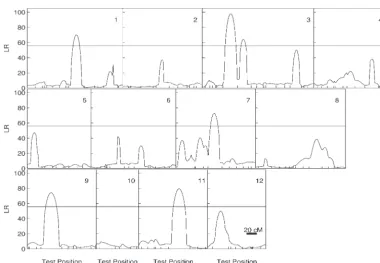
Figure 3.—The profiles of the log-likelihood ratios (LR) between the full model (there is a QTL) and reduced model (there is no QTL) for rice height growth trajectories throughout the rice genome composed of 12 chromosomes (10). The genomic position corre-sponding to the peak of the curve is the maximum-likeli-hood estimate of the QTL location. Tick marks on the x-axis represent the posi-tions of microsatellite mark-ers on each chromosome (bar, 20 cM). The map dis-tances between two markers are calculated using the Haldane mapping function. The critical thresholds for acclaiming the genome-wide existence of a QTL are ob-tained from permutation tests. The 99.9th percentile (indicated at horizonal lines) of the distribution of the maximum LR values ob-tained from 1000 permuta-tion tests is used as an empir-ical critempir-ical value to declare genome-wide existence of a QTL at␣ ⫽0.001.
growth equation. However, this equation does not nec- constant variance for the AR(1) model may not be true
in our data, as indicated by increased variance with ages essarily work better in practice than the reduced logistic
equation (k⫽2) because the former contains one more in both locations (Figure 2).Wuet al.(2004b) proposed
a transformation approach, called the transform-both-parameter than the latter. If both the equations provide
a similar likelihood of the data, the parsimonious logis- sides (TBS) model by Carroll andRuppert (1984),
to reduce variance heteroscedasticity and, therefore, tic equation should be used. In this example, the logistic
equation is sufficient to fit our growth data and, there- increase the power of the model. This TBS-based
map-ping model can also preserve the biological meanings fore, is employed to search for growth QTL through a
genome-wide scanning approach. The assumption of of curve parameters. In this study, we incorporate the
TBS-based model through log-transformation into the
functional mapping framework for analyzing QTL ⫻
TABLE 1
location interactions. As shown in Figure 2, C and D,
The conditional probabilities of QTL genotypes given the log-transformation can lead to relatively constant genotypes of two molecular markers bracketing variances in plant height growth at both locations, al-the QTL in a backcross population though a more effective transformation approach should
be estimated simultaneously with the model parameters
QTL genotype
(BoxandCox1964;CarrollandRuppert1984).
Marker genotype Q Q qq By comparing with the genome-wide critical thresh-old determined by permutation tests, we detected five
MᐉmᐉMᐉ⫹1mᐉ⫹1 1 0
significant QTL (P⬍ 0.001) on chromosomes 1, 3, 7,
Mᐉmᐉmᐉ⫹1mᐉ⫹1 1⫺ 1
9, and 11 that were responsible for growth trajectories
mᐉmᐉMᐉ⫹1mᐉ⫹1 1 1⫺
of plant heights (Figure 3). The estimated locations of
mᐉmᐉmᐉ⫹1mᐉ⫹1 0 1
these QTL correspond to the genome positions showing
No double recombination is assumed. ⫽ r1/r, where r1
the maximum-log-likelihood-ratio test statistics. Table 1
and rare the recombination fractions between marker ᏹᐉ
gives the estimates of the positions of the detected QTL
and the QTL as well as between the two flanking markersMᐉ
Figure4.—Four growth curves of the QTL ge-notypes for the QTL detected on different chro-mosomes for rice plants grown in two contrasting locations (Hangzhou, red curves, and Hainan, blue curves). The solid curves represent QTL ge-notypesQQ, whereas the broken curves represent QTL genotypeqq. AlleleQis the allele inherited from the tall Azucena parent and alleleqis inher-ited from the short IR64 parent.
chromosomes, as well as the estimates of the curve and on growth. As indicated by two divergent curves each
representing a different QTL genotype,QQorqq, the
de-matrix-structuring parameters.
We drew the age-dependent expression profiles of two tected QTL exhibited increasing effects on plant height
in both locations as rice grows. The difference between different QTL genotypes for each QTL identified from
our model for plant heights grown in Hangzhou and the areas under the growth curves of different genotypes
reflects the influence of the QTL on the overall growth Hainan (Figure 4). These profiles were drawn using the
MLEs of growth curve parameters given in Table 2. The process of plant height. We use Equation 13 to test
whether a QTL interacts with locations to affect entire profiles of gene expression allow for the
characteriza-tion of the developmental timing for a QTL to turn on growth trajectories. The test result indicated that none
of the five detected QTL displayed significant genotype⫻
or turn off or the period for the QTL to trigger its effect
TABLE 2
The MLEs of the QTL position, QTL effects described by growth parametersᏳjl⫽(ajl,bjl,rjl), residual variance (l), and correlation (l) in two different locations
Q Q qq Residual
Marker interval a2l b2l c2l a0l b0l c0l 2l l
Chromosome 1
Hangzhou RG146-RG345 149.3 2.9667 0.3100 103.5 2.2418 0.3222 0.0164 0.7274
Hainan 125.6 3.9509 0.3688 90.3 3.7650 0.3439 0.0249 0.7479
Chromosome 3
Hangzhou RZ678-RZ574 149.9 2.8989 0.3025 104.7 2.3095 0.3244 0.0161 0.7325
Hainan 128.0 4.0358 0.3634 91.0 3.7509 0.3451 0.0249 0.7529
Chromosome 7
Hangzhou PGMS0.7-CDO59 103.5 2.2148 0.3367 153.0 3.0282 0.3011 0.0175 0.7412
Hainan 82.1 3.2240 0.4143 135.1 4.3052 0.3437 0.0276 0.7808
Chromosome 9
Hangzhou RZ206-RZ422 154.3 3.0062 0.3093 106.8 2.3113 0.3281 0.0174 0.7413
Hainan 130.0 3.9470 0.3707 91.1 3.5561 0.3602 0.0256 0.7635
Chromosome 11
Hangzhou RG247-RG103 161.6 3.1405 0.3032 109.8 2.3272 0.3262 0.0181 0.7516
environment interactions, suggesting that they are more ecology, and evolution. With this new strategy, two major challenging questions in contemporary developmental general growth regulators. Using the hypothesis test in
Equation 15, we found that the time-specific growth QTL biology can be well addressed, which regard the
exis-tence of particular regulatory genes guiding growth dif-detected on chromosomes 1, 3, 9, and 11 are expressed
ferentiation during an entire biological process and the consistently stronger in Hangzhou than in Hainan,
alteration of the genetic architecture of a complex trait whereas the QTL on chromosome 7 displayed an
oppo-over developmental times. site expression pattern (Figure 4). As expected, at all
In this article, we extended our theoretical model the QTL, except for one on chromosome 7, the tall
for functional mapping to study dynamic patterns of Azucena parent contributes height-increasing alleles in
genetic effects of QTL governing growth curves and both locations, whereas the short IR64 parent
contrib-unravel the genetic machinery of organismic responses utes height-decreasing alleles.
to different environments during the course of growth Adult height for rice can be genetically controlled
and development. This extended model was employed during an early stage of development by mapping the
to study the genetic architecture of plant height growth QTL determining the timing of maximum growth rate.
trajectories in a plant model system—rice. We have suc-Such early genetic manipulation for height growth can
cessfully detected five QTL on different chromosomes potentially preserve more energy for later reproductive
that exert significant impacts on growth processes, with propagation. The significant QTL detected for overall
similar patterns across sharply contrasting environments. growth trajectories were all observed to affect the timing
At four QTL, the tall parents contribute most favorable of maximum height growth rate (inflection point;
Fig-alleles to their progeny at these detected QTL. All these ure 4), all of which, except for the one on chromosome
five QTL are expressed differently throughout entire
7, displayed significant genotype⫻environment
inter-growth processes between the two environments. These
action effects on this timing (P⬍0.001). The QTL on
results suggest that it is possible to make efficient chromosomes 1, 3, 9, and 11 trigger significant effects
marker-assisted selection for rice varieties with reduced-on the timing of maximum growth rate for rice grown
height growth and, therefore, stronger resistance to wind in Hangzhou, whereas no such effects were detected
and rain damage and higher grain yields through allocat-for Hainan.
ing more resources to the reproductive organs than to
vegetative tissues (Sakamotoet al.2003).
In a comparison with previous results for growth QTL
DISCUSSION
based on the same material by traditional interval
map-The advent of powerful genetic and molecular tools ping (Yanet al.1998), we have several interesting
find-has made it possible to define the machinery of develop- ings. First, Yanet al.detected 11 QTL for plant height
ment in terms of gene action and interaction of individ- growth in rice. Many of these QTL were not detected
ual loci or QTL (Cheverudet al.1996;Yanet al.1998). by our functional mapping model, but do display clear,
A number of statistical methods have been proposed to although nonsignificant, peaks in our LR profile (Figure
map QTL underlying complex phenotypes primarily on 3). For example, Yanet al. detected a QTL bracketed
the basis of goodness of fit to observational data rather by markers Amy3D and E-RZ66 on chromosome 8 where
than on the basis of any biological mechanism (Lander our LR profile displays a peak. But according to our
andBotstein 1989). However, the degree of the suc- criterion, this QTL is not significant. This discrepancy
cessful identification of QTL depends on the power may be due to the low criterion these authors have used.
of QTL mapping techniques to analyze growth data Second, many QTL detected from our model were not
measured at many different time points and, more im- detected by traditional interval mapping (Yanet al.1998).
portantly, on the construction of a conceptual framework But all of our QTL were detected to exist at similar
loca-for integrating biological principles of growth laws into tions for different rice materials with a larger sample
developmental processes through powerful statistical size (Liet al.2003). For example, Liet al.found a
signifi-models. cant plant height QTL between RG345 and RG381 on
We have framed a new statistical strategy for QTL map- chromosome 1 that fails to be detected by Yanet al.but
ping through specific incorporation of biological laws is supported by our model. This may suggest that our
behind the phenotypic expression of complex traits. model displays greater power to detect growth QTL of
The new strategy, termedfunctional mapping(Maet al. small effects. Third, as discussed inMaet al.(2002) and
2002; Wu et al. 2002a), displays greater potential for Wuet al.(2004a), our functional mapping
incorporat-improving the precision, power, and resolution of QTL ing developmental principles allows for the tests of a
mapping in any organism, as compared with traditional number of biologically meaningful hypotheses at
inter-mapping approaches (Maet al.2002). Functional map- play between genetics and development.
ping grounds theoretical genetic models in integrated Growth for all organisms undergoes complex
devel-developmental networks or processes and, consequently, opmental stages. For example, rice growth includes
ics, conditional epigenetic variability and growth in mice.
Genet-(panicle initiation to heading), and grain filling and
ripen-ics147:765–776.
ing or maturation (heading to maturity;Moldenhauer Box, G. E. P., andD. R. Cox, 1964 An analysis of transformations.
and Slaton 2003). Each of these stages determines J. R. Stat. Soc. Ser. B26:211–252.
Carroll, R. J., andD. Ruppert, 1984 Power-transformations when
grain yield by influencing the number of panicles per
fitting theoretical models to data. J. Am. Stat. Assoc.79:321–328.
unit land area, the average amount of grain produced Cheverud, J. M., E. J. Routman, F. Duarte, B. van-Swinderen, K.
per panicle, and the average weight of the individual Cothranet al., 1996 Quantitative trait loci for murine growth.
Genetics142:1305–1319.
grains. Our model can detect the genetic control of QTL
Churchill, G. A., and R. W. Doerge, 1994 Empirical threshold
over the length of any of these stages and any development values for quantitative trait mapping. Genetics138:963–971.
events. Coupled with the physiological and develop- Diggle, P. J., P. Heagerty, K. Y. LiangandS. L. Zeger, 2002
Analy-sis of Longitudinal Data. Oxford University Press, Oxford.
mental changes in various stages, our model will gain
Gregorczyk, A. R., 1998 Plant growth model. J. Agron. Crop Sci.
better insights into the mechanistic bases of seed forma- 181:243–247.
tion and grain yield regulation. Huang, N., A. Parco, T. Mew, G. Magpantay, S. McCoughet al.,
1997 RFLP mapping of isozymes, RAPD and QTLs for grain
Our model also has great implications for
evolution-shape, brown planthopper resistance in a doubled haploid rice
ary studies. The evolution of complex organisms such
population. Mol. Breed.3:105–113.
as animals and plants does not occur by direct transfor- Jaffre´zic, F., andS. D. Pletcher, 2000 Statistical models for
esti-mating the genetic basis of repeated measures and other
function-mation of adult ancestors into adult descendants. Rather,
valued traits. Genetics156:913–922.
any evolutionary change includes modifications or
al-Jansen, R. C., 2000 Quantitative trait loci in inbred lines, pp. 567–
terations of a series of developmental events occurring 597 inHandbook of Statistical Genetics, edited by D. J.Balding, M.
Bishopand C.Cannings. Wiley, New York.
at different time periods during ontogeny (Rice1997).
Kirkpatrick, M., W. G. HillandR. Thompson, 1994 Estimating the
The synthesization of this fundamentally important
argu-covariance structure of traits during growth and aging, illustrated
ment into the evo-devo framework (Raff 2000; Arthur with lactation in dairy cattle. Genet. Res.64:57–69.
Lander, E. S, andD. Botstein, 1989 Mapping Mendelian factors
2002) needs knowledge of how genetic factors regulate
underlying quantitative traits using RFLP linkage maps. Genetics
developmental processes in an organism from embryo
121:185–199.
to adult to better adapt itself to different environments. Li, Z. K., S. B. Yu, R. Lafitte, N. Huang, B. Courtoiset al., 2003
While in the past the dynamic change of genetic con- QTL⫻environment interactions in rice. I. Heading date and
plant height. Theor. Appl. Genet.108:141–153.
trol over time was estimated by traditional
quantita-Ma, C. X., G. CasellaandR. L. Wu, 2002 Functional mapping of
tive genetic approaches that partition total genetic vari- quantitative trait loci underlying the character process: a
theoreti-ances into additive, dominant, and/or epistatic variance cal framework. Genetics161:1751–1762.
Ma, C. X., R. L. WuandG. Casella, 2004 FunMap: functional
components (Atchley1984;Kirkpatricket al. 1994;
mapping of complex traits. Bioinformatics20:1808–1811.
Atchleyand Zhu 1997; Pletcher and Geyer1999; Mackay, T. F. C., 2001 Quantitative trait loci inDrosophila.Nat. Rev.
Jaffre´zicandPletcher2000), our functional mapping Genet.2:11–20.
Moldenhauer, K., andN. Slaton, 2003 Rice growth and
develop-model demonstrates tremendous power to precisely
char-ment, pp. 7–14 inRice Production Handbook. Cooperative
Exten-acterize these genetic components at any particular devel- sion Service, University of Arkansas, Little Rock, AR.
opmental stages and relate them to the genetic control Nath, S. R., andF. D. Moore, III, 1992 Growth analysis by the first,
second, and third derivatives of the Richards function. Growth
mechanisms for other life-history traits. With this model,
Dev. Aging56:237–247.
we are closer to addressing historically difficult ques- Niklas, K. L., 1994 Plant Allometry: The Scaling of Form and Process.
tions of how small genotypic modifications are trans- University of Chicago, Chicago.
Piepho, H.-P., 2000 A mixed-model approach to mapping
quantita-lated into phenotypic changes during evolution and
tive trait loci in barley on the basis of multiple environment data.
how microevolutionary changes contribute to macro- Genetics
156:2043–2050.
evolutionary events. Our model presented in this article Pletcher, S. D., andC. J. Geyer, 1999 The genetic analysis of
age-dependent traits: modeling the character process. Genetics153:
is being implemented in our web-based software, called
825–835.
FunMap (Ma et al. 2004), to facilitate other scientists’
Raff, R. A., 2000 Evo-devo: the evolution of a new discipline. Nat.
investigations of the genotype⫻ environment interac- Rev. Genet.1:74–79.
Rice, S. H., 1997 The analysis of ontogenetic trajectories: when a
tions for growth trajectories.
change in size or shape is not heterochrony. Proc. Natl. Acad.
We thank three anonymous reviewers for their constructive com- Sci. USA94:907–912.
ments on the article that led to a better presentation of it. The prepara- Richards, F. J., 1959 A flexible growth function for empirical use.
tion of this article is supported by the University of Florida Research J. Exp. Bot.10:290–300.
Opportunity Fund (02050259) to R.W. The publication of this article Sakamoto, T., Y. Morinaka, K. Ishiyama, M. Kobayashi, H. Itoh
et al., 2003 Genetic manipulation of gibberellin metabolism in is approved as journal series R-08963 by the Florida Agricultural
Exper-transgenic rice. Nat. Biotechnol.21:909–913.
iment Station.
Vieira, C., E. G. Pasyukova, Z-B. Zeng, J. B. Hackett, R. F. Lyman et al., 2000 Genotype-environment interaction for quantitative
trait loci affecting lifespan in Drosophila melanogaster. Genetics
154:213–227.
LITERATURE CITED
von Bertalanffy, L., 1957 Quantitative laws for metabolism and
growth. Q. Rev. Biol.32:217–231.
Arthur, W., 2002 The emerging conceptual framework of
evolu-West, G. B., J. H. BrownandB. J. Enquist, 1997 A general model
tionary developmental biology. Nature415:757–764.
for the origin of allometric scaling laws in biology. Science276:
Atchley, W. R., 1984 Ontogeny, timing of development, and
ge-122–126.
netic variance-covariance structure. Am. Nat.123:519–540.
dimension of life: fractal geometry and allometric scaling of or- Wu, R. L., C.-X. Ma, M. Lin andG. Casella, 2004a A general framework for analyzing the genetic architecture of
develop-ganisms. Science284:1677–1679.
mental characteristics. Genetics166:1541–1551.
West, G. B., J. H. BrownandB. J. Enquist, 2001 A general model
Wu, R. L., C.-X. Ma, M. Lin, Z. H. WangandG. Casella, 2004b
for ontogenetic growth. Nature413:628–631.
Functional mapping of quantitative trait loci underlying growth
Wu, R. L., 1998 The detection of plasticity genes in heterogeneous
trajectories using a transform-both-sides logistic model.
Biomet-environments. Evolution52:967–977.
rics60:729–738.
Wu, R. L., Z-B. Zeng, S. E. McKendandD. M. O’Malley, 2000 The
Yan, J.-Q., J. Zhu, C.-X. He, M. BenmoussaandP. Wu, 1998 Molecu-case for molecular mapping in forest tree breeding. Plant Breed.
lar dissection of developmental behavior of plant height in rice
Rev.19:41–68.
(Oryza sativaL.). Genetics150:1257–1265.
Wu, R. L., C.-X. MaandG. Casella, 2002a Joint linkage and linkage
Zhao, W., C. Ma, J. M. CheverudandR. L. Wu, 2004 A unifying disequilibrium mapping of quantitative trait loci in natural
popu-statistical model for QTL mapping of genotype⫻sex interaction
lations. Genetics160:779–792.
for developmental trajectories. Physiol. Genomics19:218–227.
Wu, R. L., C.-X. Ma, M. Chang, R. C. Littell, S. S. Wuet al., 2002b
Zimdahl, H., T. Kreitler, C. Gosele, D. GantenandN. Hubner,
A logistic mixture model for characterizing genetic determinants 2002 Conserved synteny in rat and mouse for a blood pressure
causing differentiation in growth trajectories. Genet. Res. 79: QTL on human chromosome 17. Hypertension39:1050–1052.
235–245. Zimmerman, D. L., andV. Nu´ n˜ ez-Anto´ n, 2001 Parametric modeling
Wu, R. L., C. X. Ma, M. C. K. Yang, M. Chang, U. Santraet al., of growth curve data: an overview. Test10:1–73.
2003 Quantitative trait loci for growth in Populus. Genet. Res.