Influence of Mom and Dad: Quantitative Genetic Models for Maternal Effects and Genomic Imprinting

DOI: 10.1534/genetics.105.049494

Influence of Mom and Dad: Quantitative Genetic Models for Maternal

Effects and Genomic Imprinting

Anna W. Santure

_{and Hamish G. Spencer}

Allan Wilson Centre for Molecular Ecology and Evolution, Department of Zoology, University of Otago, Dunedin, 9001 New Zealand

Manuscript received August 11, 2005 Accepted for publication May 29, 2006

ABSTRACT

The expression of an imprinted gene is dependent on the sex of the parent it was inherited from, and as a result reciprocal heterozygotes may display different phenotypes. In contrast, maternal genetic terms arise when the phenotype of an offspring is influenced by the phenotype of its mother beyond the direct inheritance of alleles. Both maternal effects and imprinting may contribute to resemblance between offspring of the same mother. We demonstrate that two standard quantitative genetic models for deriving breeding values, population variances and covariances between relatives, are not equivalent when maternal genetic effects and imprinting are acting. Maternal and imprinting effects introduce both sex-dependent and generation-sex-dependent effects that result in differences in the way additive and dominance effects are defined for the two approaches. We use a simple example to demonstrate that both imprinting and maternal genetic effects add extra terms to covariances between relatives and that model misspecification may over- or underestimate true covariances or lead to extremely variable parameter estimation. Thus, an understanding of various forms of parental effects is essential in correctly estimating quantitative genetic variance components.

A

Tilghman 1997). Some 83 transcriptional units are

currently known to be imprinted in mammals (Morison

et al. 2005). Complete inactivation of an imprinted gene

results in functional haploidy, with only one of the two copies of a gene expressed. For example, insulin-like growth factor 2 (Ig f2) is expressed only from the paternal allele in most fetal tissues of eutherian and marsupial mammals (DeChiaraet al. 1991; O’Neill et al. 2000).

More generally, however, imprinting results in the func-tional nonequivalence of reciprocal heterozygotes, where inheriting anA1allele from one’s mother and anA2 al-lele from one’s father gives a different phenotype, on av-erage, than the reverse inheritance pattern.

Maternal effects arise when the genetic and environ-mental characteristics of a mother influence the phe-notype of her offspring, beyond the direct inheritance of alleles. These effects contribute to resemblance be-tween offspring of the same mother, and bebe-tween mothers and their offspring, and are extensively recog-nized in traits such as offspring growth, production, and

disease risk (Wade1998). For example, significant

ma-ternal effects for early growth in mice were detected in a QTL mapping study (Wolf et al. 2002). Maternal

genetic effects contribute an extra term in addition to an offspring’s own genotypic value, dependent on the genotype of the mother (Lynchand Walsh1998). This

effect on offspring phenotype is also termed an indirect genetic effect, as the maternal phenotype (itself de-termined by genetic factors) acts as an environmental influence on offspring phenotype (Mooreet al. 1998).

Such indirect genetic effects increase resemblances between mothers and offspring and between siblings. Maternal effects may also arise independently of genetic factors. For example, Hucket al. (1987) demonstrated

that food restriction in the early life of golden hamsters,

Mesocricetus auratus, leads to reduced numbers and

female-biased sex ratios in litters borne later in life. Further, a nongenetic influence need not be restricted to a maternal environmental effect—the father’s envi-ronmental conditions may also contribute to the char-acteristics of offspring (Shawand Byers1998).

For quantitative traits, it may be difficult to distin-guish maternal genetic effects from imprinting effects. For example, both maternal effects and genomic im-printing can increase the covariance between the geno-typic values of mothers and their offspring (Kempthorne

1957; Spencer2002). It is therefore of interest to

de-rive a quantitative genetic model to incorporate both imprinting and maternal genetic effects (hereafter termed maternal effects) to discover if these distinct

1_{Corresponding author:Allan Wilson Centre for Molecular Ecology and}

Evolution, Department of Zoology, University of Otago, P.O. Box 56, Dunedin, 9001 New Zealand. E-mail: [email protected]

causative processes lead to differences in population statistics.

THE MODEL

We combine standard quantitative genetic models for additive maternal genetic effects (Kempthorne1957)

and genomic imprinting (Spencer 2002) to calculate

breeding values, genetic variances, and covariances be-tween relatives. Following the approach of Spencer

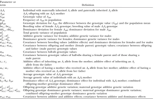
(2002), consider an autosomal two-allele locus with al-lelesA1andA2at frequencyp1andp2, respectively, in the population. We write the maternally inherited allele first, such thatA2A1has a maternally inheritedA2allele and a paternally inheritedA1allele. LetAijklrepresent anAiAjoffspring with anAkAlmother andGijklrepresent the genotypic value ofAijkl. Note that important param-eters and notation introduced in this text are also summarized in Table 1.

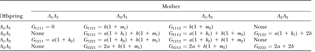
Table 2 shows all possible genotypic values for off-spring, given the genotype of their mother. Here 0,a(11

k1), a(1 1 k2), and 2a represent genotypic contribu-tions fromA1A1,A2A1,A1A2, andA2A2offspring and 0,

b(1 1 m1), b(1 1 m2), and 2b represent genotypic contributions fromA1A1,A2A1,A1A2, andA2A2mothers.

For example, anA2A1offspring with anA1A2mother has a genotypic valueG2112¼a(11k1)1b(11m2), with

a(11 k1) representing the contribution from its own genotype andb(11m2) representing the contribution to genotypic value from its mother’s genotype. Follow-ing Spencer (2002), genomic imprinting is included

in the model by assigning separate genotypic contribu-tions for the reciprocal heterozygotesA2A1andA1A2by use of the parametersk1andk2andm1andm2. Note that in the absence of imprintingk1¼k2andm1¼m2, while in the absence of maternal effectsb¼0 (and hencem1¼

m2¼0 also).

The classical definition for imprinting, complete inac-tivation of one allele, corresponds tok1 ¼ 1 andk2¼1 andm1¼ 1 andm2¼1 (complete silencing of the ma-ternal allele) or k1¼1 andk2¼ 1 andm1¼1 and

m2¼ 1 (complete silencing of the paternal allele). More recently, however, imprinting has been treated as a quantitative trait, which implies that maternal or pater-nal alleles may be only partially inactivated (see, e.g., Sandovici et al. 2003, 2005; Naumova and Croteau

2004), andk1,k2,m1, andm2may take any value in the range½1;1.

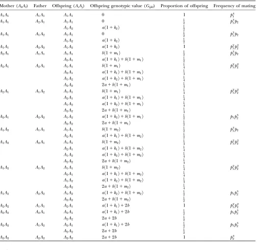
Table 3 shows the complete array of offspring ge-notypes and their frequency in the population from TABLE 1

Definition of parameters and notation used in text

Parameter or

term Definition

AiAj Individual with maternally inheritedAiallele and paternally inheritedAjallele

Aijkl AiAjoffspring with anAkAlmother

Gijkl Genotypic value ofAijkl

frijkl Frequency ofAijklin population

gdijkl Genotypic deviation forAijkl, the difference between the genotypic value (Gijkl) and the population mean

bvfij;bvmij Breeding value of femaleAiAjgenotype; breeding value of maleAiAjgenotype

ddfijkl;ddmijkl Dominance deviation for femaleAijkl; dominance deviation for maleAijkl s2

G Total genetic variance of population

s2 Af;s

2

Am Additive genetic variance for females; additive genetic variance for males s2

Df;s 2

Dm Dominance genetic variance for females; dominance genetic variance for males

sADf;sADm Covariance between breeding values (additive effects) and dominance deviations for females and for males sOPf;sOPm Covariance between offspring and mother (female parent) genotypic values; covariance between offspring

and father (male parent) genotypic values sFS Covariance between full-sib genotypic values

sHSf;sHSm Covariance between genotypic values of half-sibs sharing a female parent and of those sharing a

male parent

ei:;e:j Additive effect of inheriting anAiallele from the mother; additive effect of inheriting anAj

allele from the father

vk:;v:l Additive effect of having a mother who received anAkallele from her mother; additive effect of having a

mother who received anAlallele from her father

Gij:: Average genotypic value ofAiAjgenotype

G::kl Average genetic value of individuals with anAkAlmother

lij;ukl;dijkl Dominance effect ofAiAjgenotype; dominance effect for individual withAkAlmother; combined

offspring–mother genotype dominance effect s2

AðeÞ;s2AðvÞ Offspring genotype additive genetic variation; maternal genotype additive genetic variation s2

DðlÞ;s 2 DðuÞ;s

2

DðdÞ Offspring genotype dominance genetic variance; maternal genotype dominance genetic variation;

combined offspring–mother genotype dominance genetic variation

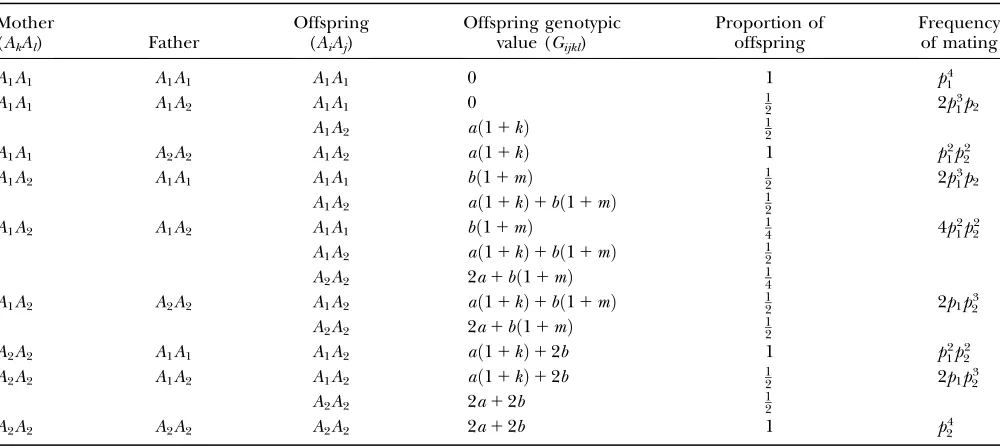
each possible parent mating combination. Returning to Tables 2 and 3, note that a number of mother–offspring combinations are not possible without introducing mutation—for example, it is not possible for an A1A1 mother to produce anA2A1offspring.

With the help of Table 3, the mean genotypic value over the population is

m¼ X

offspring genotypes

genotypic value3proportion3frequency of mating

¼p2ðað21p1ðk11k2ÞÞ1bð21p1ðm11m2ÞÞÞ: ð1Þ

When maternal effects are zero (that is,b¼0), the mean genotypic value is identical to that under imprinting alone (Spencer 2002). Similarly with no imprinting

(k1¼k2¼kand m1¼m2¼m) the mean reduces to

m¼2p2ðað11kp1Þ1bð11mp1ÞÞ, the equivalent expres-sion in Kempthorne’s (1957) model.

We follow a number of approaches in calculating breeding values, components of variance, and covari-ances between relatives. Doing so illustrates that various assumptions made in these approaches are not valid in the presence of imprinting and maternal effects.

Approach 1:We first follow the approach of Falconer

and Mackay (1996) and Kempthorne (1957), using

genotypic values of parents and offspring to calcu-late population breeding values, dominance deviations, components of variance, and covariances between relatives.

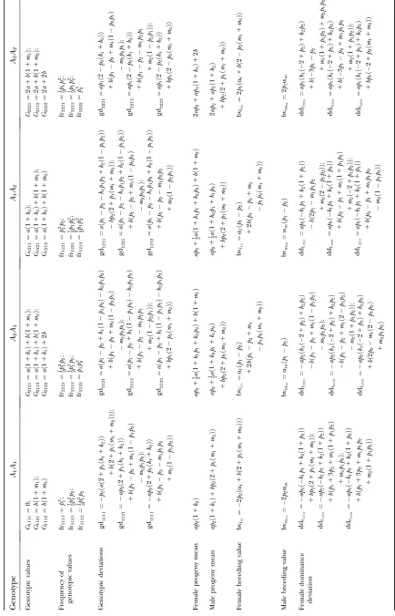
We begin by calculating the frequency, frijkl, of each genotype,Aijkl(Table 4), by summing over the product of mating frequencies and proportion of offspring for eachAijklfrom Table 3. For example (from Table 3),

fr1221¼1₄p21p22114p 2

1p22112p1p 3 2

¼1

2p1p 2 2:

We now calculate genotypic deviations (gdijkl) for each

Aijkl, the difference between the genotypic value (Gijkl)

and the population mean; the values are shown in Table 4. Note that genotypic deviations are calculated sepa-rately for each Aijkl and should not be averaged over mothers.

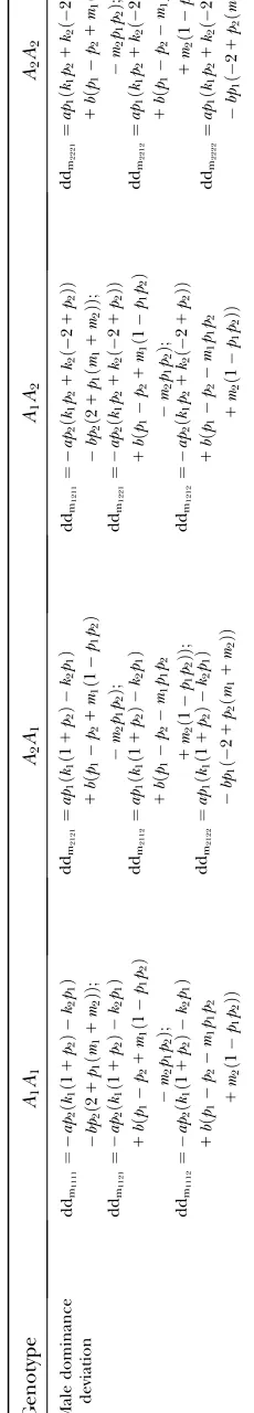
Breeding values for eachAiAjgenotype are defined as twice the difference between the mean genotypic

value of that class’s offspring and the population mean (Falconer and Mackay 1996). Progeny means are

included in Table 4. Unlike genotypic values and deviations, progeny means and breeding values need not be calculated separately for genotypes with different maternal genotypes (i.e., for allAijkl), but do need to be calculated separately for males (bvmij) and females (bvfij). Breeding values are different for males and females because all offspring of a dam share the same maternal effect while offspring of a sire have four different maternal contributions. Finally, male and female dominance deviations (ddmijkl and ddfijkl), the difference between the genotypic deviation and the breeding value for each genotype, may be derived (Table 4).

Genetic variance components: The genetic variance

of the population (s2

G) is the variance of the genotypic deviations,

s2 G¼

X

ijkl

frijklgd2ijkl

¼p1p2½a2ððk1k2Þ21p1p2ðk11k2Þ2Þ

1b2ððm1m2Þ21p1p2ðm11m2Þ2Þ

12a_fa_m12b_fb_m1a_fðb_f1b_mÞ

¼p1p2½a2p1p2ðk11k2Þ21b2p1p2ðm11m2Þ2

1a2_f1a2_m1b2_f 1b_m2 1afðbf1bmÞ; ð2Þ

where, for simplicity, we define the terms

a_f ¼að11k1p1k2p2Þ;

am¼að11k2p1k1p2Þ;

b_f ¼bð11m1p1m2p2Þ; and

b_m¼bð11m2p1m1p2Þ:

In the absence of maternal effects (b¼0), the total variance is equivalent to that under imprinting alone (Spencer2002).

Note that whenk1¼k2¼kandm1¼m2¼m, so that imprinting is absent, Equations 1 and 2 reduce to

m¼2p2ðað11kp1Þ1bð11mp1ÞÞ ð3Þ

TABLE 2

Genotypic values for offspring dependent on the genotype of their mother

Mother

Offspring A1A1 A2A1 A1A2 A2A2

A1A1 G1111¼0 G1121¼b(11m1) G1112¼b(11m2) None

A2A1 None G2121¼a(11k1)1b(11m1) G2112¼a(11k1)1b(11m2) G2122¼a(11k1)12b

A1A2 G1211¼a(11k2) G1221¼a(11k2)1b(11m1) G1212¼a(11k2)1b(11m2) None

and

s2_G¼2p1p2½2p1p2ða2k21b2m2Þ1a21ab1b2; ð4Þ wherea¼að11kðp1p2ÞÞandb¼bð11mðp1p2ÞÞ. These are equivalent to the values of Kempthorne

(1957), using our notation (see Table 5 for the mating table showing all possible offspring genotypes for mater-nal effects in the absence of imprinting and Table 6 for genotypic values, breeding values, and dominance deviations under maternal effects alone).

The additive genetic variances for females (s2 Af) and males (s2

Am) are the respective variances of their breed-ing values:

s2_A

f ¼

X2

i;j¼1

pipjbv2fij

¼2p1p2½b2ððm1m2Þ212p1p2ðm11m2Þ2Þ

1ða_f1b_f1b_mÞ2 _ð5Þ

and

s2_A

m ¼

X2

i;j¼1

pipjbv2mij

¼2p1p2a2m: ð6Þ

TABLE 3

Mating table of all possible offspring genotypes under imprinting and maternal effects

Mother (AkAl) Father Offspring (AiAj) Offspring genotypic value (Gijkl) Proportion of offspring Frequency of mating

A1A1 A1A1 A1A1 0 1 p41

A1A1 A2A1 A1A1 0 1₂ p31p2

A1A2 að11k2Þ 1₂

A1A1 A1A2 A1A1 0 1₂ p31p2

A1A2 að11k2Þ 1₂

A1A1 A2A2 A1A2 að11k2Þ 1 p21p22

A2A1 A1A1 A1A1 bð11m1Þ 1₂ p31p2

A2A1 að11k1Þ1bð11m1Þ 1₂

A2A1 A2A1 A1A1 bð11m1Þ 14 p21p22

A2A1 að11k1Þ1bð11m1Þ 1₄

A1A2 að11k2Þ1bð11m1Þ 1₄

A2A2 2a1bð11m1Þ 14

A2A1 A1A2 A1A1 bð11m1Þ 1₄ p21p

2 2

A2A1 að11k1Þ1bð11m1Þ 1₄

A1A2 að11k2Þ1bð11m1Þ 1₄

A2A2 2a1bð11m1Þ 1₄

A2A1 A2A2 A1A2 að11k2Þ1bð11m1Þ 1₂ p1p32

A2A2 2a1bð11m1Þ 1₂

A1A2 A1A1 A1A1 bð11m2Þ 1₂ p31p2

A2A1 að11k1Þ1bð11m2Þ 1₂

A1A2 A2A1 A1A1 bð11m2Þ 1₄ p21p22

A2A1 að11k1Þ1bð11m2Þ 1₄

A1A2 að11k2Þ1bð11m2Þ 1₄

A2A2 2a1bð11m2Þ 1₄

A1A2 A1A2 A1A1 bð11m2Þ 1₄ p21p

2 2

A2A1 að11k1Þ1bð11m2Þ 1₄

A1A2 að11k2Þ1bð11m2Þ 1₄

A2A2 2a1bð11m2Þ 1₄

A1A2 A2A2 A1A2 að11k2Þ1bð11m2Þ 1₂ p1p32

A2A2 2a1bð11m2Þ 1₂

A2A2 A1A1 A2A1 að11k1Þ12b 1 p21p22

A2A2 A2A1 A2A1 að11k1Þ12b 1₂ p1p32

A2A2 2a12b 1₂

A2A2 A1A2 A2A1 að11k1Þ12b 1₂ p1p32

A2A2 2a12b 1₂

T ABLE 4 Genotypic values, frequencies, breeding values, and dominance deviations for imprinting and additive mater nal-ef fects model Genotype A1 A1 A2 A1 A1 A2 A2 A2 Genotypic values G1111 ¼ 0 ; G1121 ¼ b ð 1 1 m1 Þ ; G1112 ¼ b ð 1 1 m2 Þ G2121 ¼ a ð 1 1 k1 Þ 1 b ð 1 1 m1 Þ ; G2112 ¼ a ð 1 1 k1 Þ 1 b ð 1 1 m2 Þ ; G2122 ¼ a ð 1 1 k1 Þ 1 2 b G1211 ¼ a ð 1 1 k2 Þ ; G1221 ¼ a ð 1 1 k2 Þ 1 b ð 1 1 m1 Þ ; G1212 ¼ a ð 1 1 k2 Þ 1 b ð 1 1 m2 Þ G2221 ¼ 2 a 1 b ð 1 1 m1 Þ ; G2212 ¼ 2 a 1 b ð 1 1 m2 Þ ; G2222 ¼ 2 a 1 2 b Frequency o f genotypic values fr1111 ¼ p

3;1

fr1121

¼

1p2 2p1

2

;

fr1112

¼

1p2 2p1

2

fr2121

¼

1p2 2p1

2

;

fr2112

¼

1p2 2p1

2 ; fr2122 ¼ p1 p 2 2 fr1211 ¼ p

2p1

2

;

fr1221

¼

1p2

1

p

2;2

fr1212

¼

1p2

1

p

2 2 fr2221

¼

1p2

1

p

2;2

fr2212

¼

1p2

1

p

2;2

fr2222 ¼ p 3 2 Genotypic deviations gd 1111 ¼ p2 ð a ð 2 1 p1 ð k1 1 k2 ÞÞ 1 b ð 2 1 p1 ð m1 1 m2 ÞÞÞ ; gd 1121 ¼ ap 2 ð 2 1 p1 ð k1 1 k2 ÞÞ 1 b ð p1 p2 1 m1 ð 1 p1 p2 Þ m2 p1 p2 Þ ; gd 1111 ¼ ap 2 ð 2 1 p1 ð k1 1 k2 ÞÞ 1 b ð p1 p2 m1 p1 p2 1 m2 ð 1 p1 p2 ÞÞ gd 2121 ¼ a ð p1 p2 1 k1 ð 1 p1 p2 Þ k2 p1 p2 Þ 1 b ð p1 p2 1 m1 ð 1 p2 p1 Þ m2 p2 p1 Þ ; gd 2112 ¼ a ð p1 p2 1 k1 ð 1 p1 p2 Þ k2 p1 p2 Þ 1 b ð p1 p2 m1 p2 p1 1 m2 ð 1 p2 p1 ÞÞ ; gd 2122 ¼ a ð p1 p2 1 k1 ð 1 p1 p2 Þ k2 p1 p2 Þ 1 bp1 ð 2 p2 ð m1 1 m2 ÞÞ gd 1211 ¼ a ð p1 p2 k1 p1 p2 1 k2 ð 1 p1 p2 ÞÞ bp2 ð 2 1 p1 ð m1 1 m2 ÞÞ ; gd 1221 ¼ a ð p1 p2 k1 p1 p2 1 k2 ð 1 p1 p2 ÞÞ 1 b ð p1 p2 1 m1 ð 1 p2 p1 Þ m2 p2 p1 Þ ; gd 1212 ¼ a ð p1 p2 k1 p1 p2 1 k2 ð 1 p1 p2 ÞÞ 1 b ð p1 p2 m1 p2 p1 1 m2 ð 1 p2 p1 ÞÞ gd 2221 ¼ ap 1 ð 2 p2 ð k1 1 k2 ÞÞ 1 b ð p1 p2 1 m1 ð 1 p2 p1 Þ m2 p2 p1 Þ ; gd 2212 ¼ ap 1 ð 2 p2 ð k1 1 k2 ÞÞ 1 b ð p1 p2 m1 p2 p1 1 m2 ð 1 p2 p1 ÞÞ ; gd 2222 ¼ ap 1 ð 2 p2 ð k1 1 k2 ÞÞ 1 bp 1 ð 2 p2 ð m1 1 m2 ÞÞ Female progeny mean ap 2 ð 1 1 k2 Þ ap 2 1

1a2

ð 1 1 k1 p1 1 k2 p2 Þ 1 b ð 1 1 m1 Þ ap 2 1

1a2

ð 1 1 k1 p1 1 k2 p2 Þ 1 b ð 1 1 m2 Þ 2 ap 2 1 ap 1 ð 1 1 k1 Þ 1 2 b Male progeny mean ap 2 ð 1 1 k1 Þ 1 bp2 ð 2 1 p1 ð m1 1 m2 ÞÞ ap 2 1

1a2

ð 1 1 k2 p1 1 k1 p2 Þ 1 bp2 ð 2 1 p1 ð m1 1 m2 ÞÞ ap 2 1

1a2

ð 1 1 k2 p1 1 k1 p2 Þ 1 bp2 ð 2 1 p1 ð m1 1 m2 ÞÞ 2 ap 2 1 ap 1 ð 1 1 k2 Þ 1 bp2 ð 2 1 p1 ð m1 1 m2 ÞÞ Female breeding value b

vf11

The male additive variance is equivalent to that under imprinting alone (Spencer 2002) and is therefore

unaffected by the addition of maternal effects to the model. In contrast, the female additive genetic variance is equivalent to that under imprinting alone (Spencer

2002) only when maternal effects are absent (b¼0). We may define progeny means and breeding values for maternal effects alone (i.e., in the absence of imprint-ing) (see Table 6) as described above and find that the additive genetic variances simplify to

s2_A

f ¼2p1p2½8b

2_m2_p

1p21a214ab14b2 ð7Þ and

s2_A

m ¼2p1p2a

2_{: ð8Þ}

The dominance genetic variance is the variance of the dominance deviations and is not the same for females (s2

Df) and males (s

2 Dm): s2

Df ¼ X

ijkl

frijkldd2fijkl

¼p1p2½a2ððk1k2Þ21p1p2ðk11k2Þ2Þ

14abððk1k2Þð11m2Þ 2k1p2ðm11m2Þ

1p22ðk11k2Þðm11m2ÞÞ

1b2ð62m1m214m1ðp12p2Þ14m2ð2p1p2Þ

p1p2ðm11m2Þ21m12ð3p115p2Þ

1m22ð5p113p2ÞÞ ð9Þ and

s2_D

m ¼

X

ijkl

frijkldd2mijkl

¼p1p2½a2ððk1k2Þ21p1p2ðk11k2Þ2Þ

1aðk1k2Þðbf1bmÞ

1b2ð21m₁21m2₂12ðm11m2Þðp1p2Þ

p1p2ðm11m2Þ2Þ: ð10Þ

Under imprinting alone, dominance variances are equivalent for males and females (Spencer2002). It is

interesting to note that this equivalence is lost when maternal effects are included. Taking the variance of the dominance deviations for maternal effects alone (de-fined in Table 6), we find that

s2_D

f ¼2p1p2½2a

2_k2_p

1p28abkmp1p2110b2m2p1p213b2

ð11Þ

and

s2_D

m¼2p1p2½2p1p2ða

2_k2_1b2_m2_Þ1b2_{: ð12Þ}

The nonequivalence of dominance deviation variances under imprinting and maternal effects is therefore due to differences between male and female dominance variances under maternal effects alone.

The covariances between dominance deviations and breeding values are given by

sADf ¼

X

ijkl

frijklbvfijddfijkl

¼p1p2½1₂abð61k1ð106p213m117m2Þ

k2ð416p214m2Þ1ðm11m2Þ 3ð3ðp1p2Þ

1p2ð17k13k2110p2ðk11k2ÞÞÞÞ

b2ð61m1ð512p2Þ

1m2ð712p2Þ m1m2ð114p1p2Þ 1m12ð31p22p1p2Þ

1m2

2ð31p12p1p2ÞÞ1aafðk2k1Þ

ð13Þ

and

s_ADm ¼X

ijkl

frijklbvmijddmijkl

¼p1p2am½aðk1k2Þ11₂ðbf1bmÞ: ð14Þ

Under maternal effects alone these simplify to

sADf ¼p1p2½8abkmp1p216b

2_m2_p

1p23bða12bÞ

ð15Þ

and

s_ADm ¼p1p2ab; ð16Þ and in the absence of both maternal effects and imprinting (b¼0 andk1¼k2), the covariances are zero

and breeding values and dominance deviations are uncorrelated.

Finally, it can be easily shown that

s2_G¼s2_A

f1s

2

Df12sADf

¼s2_A

m1s

2

Dm12sADm

for both maternal effects and imprinting and for ma-ternal effects alone.

It is reassuring to note that values for the population mean, variances, and covariances under maternal ef-fects alone are equivalent whether they are derived inde-pendently from Tables 5 and 6 or by substitutingk¼k1¼

k2andm¼m1¼m2into Equations 1, 2, 5, 6, 9, 10, 13, and 14.

Resemblance between relatives: We now follow the

ap-proach of Kempthorne(1957) to calculate the mother–

offspring covariance (sOPf, covariance between o ff-spring andfemaleparent) and father–offspring covari-ance (sOPm, covariance between offspring and male

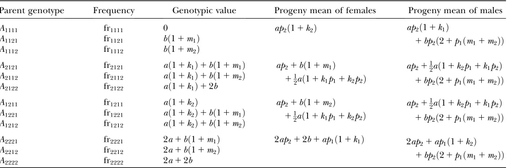
parent) using Table 7. Table 7 displays the genotypic values of parents and the mean value of offspring of these parents. Note that this table covers all 12 possi-ble parent genotypes, as it is important to not average over Akl genotypes (the male or female parent’s own mother).

Then

sOP¼

X

ijkl

frijklðGijklmÞðAijprogeny meanmÞ;

sOPf¼ 1

4p1p2½5abð21k1m11k2m2Þ 6abp1p2ðk11k2Þðm11m2Þ

12afðaf1amÞ12bfðbf1bmÞ1abmðk1k2Þ

15aðb_f1b_mÞ15bðaf1amÞ; ð17Þ and

TABLE 5

Mating table of all possible offspring genotypes under maternal effects only

Mother

(AkAl) Father

Offspring (AiAj)

Offspring genotypic value (Gijkl)

Proportion of offspring

Frequency of mating

A1A1 A1A1 A1A1 0 1 p41

A1A1 A1A2 A1A1 0 1₂ 2p31p2

A1A2 að11kÞ 1₂

A1A1 A2A2 A1A2 að11kÞ 1 p21p

2 2

A1A2 A1A1 A1A1 bð11mÞ 1₂ 2p31p2

A1A2 að11kÞ1bð11mÞ 1₂

A1A2 A1A2 A1A1 bð11mÞ 1₄ 4p21p

2 2

A1A2 að11kÞ1bð11mÞ 1₂

A2A2 2a1bð11mÞ 14

A1A2 A2A2 A1A2 að11kÞ1bð11mÞ 1₂ 2p1p32

A2A2 2a1bð11mÞ 1₂

A2A2 A1A1 A1A2 að11kÞ12b 1 p21p22

A2A2 A1A2 A1A2 að11kÞ12b 1₂ 2p1p32

A2A2 2a12b 1₂

T ABLE 6 Genotypic values, frequencies, breeding values, and dominance deviations for additive mater nal ef fects and no imprinting model Genotype A1 A1 A1 A2 ð¼ A2 A1 Þ A2 A2 Genotypic values 0 ; b ð 1 1 m Þ a ð 1 1 k Þ ; a ð 1 1 k Þ 1 b ð 1 1 m Þ ; 2 a 1 b ð 1 1 m Þ 2 a 1 b ð 1 1 m Þ ; 2 a 1 2 b Frequency of genotypic values p

3;1

p

2p1

2

p

2p1

2 ; p1 p2 ; p1 p 2 2 p1 p

2;2

p 3 2 Genotypic deviations 2 p2 ð a ð 1 1 kp 1 Þ 1 b ð 1 1 mp 1 ÞÞ ; 2 ap 2 ð 1 1 kp 1 Þ 1 b ð p1 p2 1 m ð 1 2 p1 p2 ÞÞ a ð p1 p2 1 k ð 1 2 p1 p2 ÞÞ b ð p1 p2 1 m ð 1 2 p1 p2 ÞÞ ; a ð p1 p2 1 k ð 1 2 p1 p2 ÞÞ 1 2 bp 1 ð 1 mp 2 Þ 2 ap 1 ð 1 kp 2 Þ 1 b ð p1 p2 1 m ð 1 2 p1 p2 ÞÞ ; 2 ap 1 ð 1 kp 2 Þ 1 2 bp 1 ð 1 mp 2 Þ Female progeny mean ap 2 ð 1 1 k Þ ap 2 1

1a2

ð 1 1 k Þ 1 b ð 1 1 m Þ 2 ap 2 1 ap 1 ð 1 1 k Þ 1 2 b Male progeny mean ap 2 ð 1 1 k Þ 1 2 bp2 ð 1 1 mp 1 Þ ap 2 1

1a2

ð 1 1 k Þ 1 2 bp 2 ð 1 1 mp 1 Þ 2 ap 2 1 ap 1 ð 1 1 k Þ 1 2 bp 2 ð 1 1 mp 1 Þ Female breeding value 2 p2 ð a 1 2 b ð 1 1 mp 1 ÞÞ a ð p1 p2 Þ 1 2 b ð p1 p2 1 m ð 1 2 p1 p2 ÞÞ 2 p1 ð a 1 2 b ð 1 mp 2 Þ Male breeding value 2 p2 aa ð p1 p2 Þ 2 p1 a Female dominance deviations 2 akp

212

2 bp 2 ð 1 1 mp 1 Þ ; 2 akp

212

b ð 1 1 2 p2 1 m ð 1 1 2 p1 p2 ÞÞ 2 akp 1 p2 2 b ð p1 1 m ð 1 p1 p2 ÞÞ ; 2 akp 1 p2 b ð 1 2 p2 1 m ð 1 2 p1 p2 ÞÞ ; 2 akp 1 p2 1 2 b ð p2 m ð 1 p1 p2 ÞÞ 2 akp

21

b ð 1 1 2 p1 m ð 1 1 2 p1 p2 ÞÞ ; 2 akp

21

2 bp1 ð 1 mp 2 Þ Male dominance deviations 2 akp

22

2 bp 2 ð 1 1 mp 1 Þ ; 2 akp

212

b ð p1 p2 1 m ð 1 2 p1 p2 ÞÞ 2 akp 1 p2 2 bp 2 ð 1 1 mp 1 Þ ; 2 akp 1 p2 1 b ð p1 p2 1 m ð 1 2 p1 p2 ÞÞ ; 2 akp 1 p2 2 bp 1 ð 1 mp 2 Þ ; 2 akp

211

b ð p1 p2 1 m ð 1 2 p1 p2 ÞÞ ; 2 akp

211

sOPm ¼

1

4p1p2am½2ðaf1amÞ1bf1bm: ð18Þ Note that, following Spencer(2002), these

covarian-ces are equivalent to

sOPf ¼

1 2ðs

2

Af1sADfÞ ð19Þ

and

s_OPm ¼1 2ðs

2

Am1sADmÞ: ð20Þ

The full-sib covariance (sFS) can be calculated with the aid of Table 8, which displays all possible genotypic values and frequencies of pairs of siblings:

sFS¼

X

offspring pairs

frðoffspringGijklmÞðoffspringGijklmÞ

¼p1p2½1₄a2p1p2ðk11k2Þ211₂ða2f1a2mÞ

1b2p1p2ðm11m2Þ21b2f1b2m1afðbf1bmÞ:

ð21Þ

In the absence of imprinting, settingk¼k1¼k2andm¼

m1¼m2, we find that

s_OPf ¼1

2p1p2½8abkmp1p212a

2_12b2_15ab;

sOPm ¼

1

2p1p2a½2a1b; and

s_FS¼p1p2½a2k2p1p214b2m2p1p21a212ab12b2: These covariances are equivalent to the values of Kempthorne (1957), using our notation (note that

his definitions fora andbare not the same as ours). When imprinting is present in the absence of maternal effects (b¼0),

sOPf ¼

1

2p1p2af½aðk2k1Þ12af;

s_OPm ¼1

2p1p2am½aðk1k2Þ12am

(also derived by Spencer2002), and

sFS¼1₄p1p2½a2p1p2ððk11k2Þ212p1ðk1k2Þð2p2ðk11k2ÞÞÞ 12ða2

f1a2mÞ:

Finally, we may also calculate the covariance between offspring who share a mother or a father. Following Spencer (2002), the covariance of half-siblings who

share a mother is

s_HSf ¼1 4s

2 Af

¼1

2p1p2½b 2_ððm

1m2Þ212p1p2ðm11m2Þ2Þ

1a2_f 12afðbf1bmÞ1ðbf1bmÞ2

ð22Þ

and the covariance of half-sibs sharing a father is

sHSm ¼

1 4s

2 Am

¼1

2p1p2a 2

m: ð23Þ

These covariances reduce to

sHSf ¼

1 2p1p2½8b

2_m2_p

1p21a214ab14b2 and

s_HSm ¼1 2p1p2a

2 in the absence of imprinting and

sHSf ¼

1 2p1p2a

2 f and

sHSm ¼

1 2p1p2a

2 m

if we assume no maternal effects (Spencer2002).

Approach 2a: We now follow a general least-squares

approach (Lynchand Walsh 1998) to calculate

pop-ulation breeding values, dominance deviations, compo-nents of variance, and covariances between relatives.

We can write the genotypic valueGijklas the sum of the mean plus the additive (eandv) and dominance (l;u;andd) effects,

TABLE 7

Genotypic values and progeny means for mother–offspring and father–offspring pairs under maternal effects and imprinting

Parent genotype Frequency Genotypic value Progeny mean of females Progeny mean of males

A1111 fr1111 0 ap2ð11k2Þ ap2ð11k1Þ

1bp2ð21p1ðm11m2ÞÞ

A1121 fr1121 bð11m1Þ

A1112 fr1112 bð11m2Þ

A2121 fr2121 að11k1Þ1bð11m1Þ ap21bð11m1Þ 11

2að11k1p11k2p2Þ

ap211₂að11k2p11k1p2Þ 1bp2ð21p1ðm11m2ÞÞ

A2112 fr2112 að11k1Þ1bð11m2Þ

A2122 fr2122 að11k1Þ12b

A1211 fr1211 að11k2Þ ap21bð11m2Þ

11

2að11k1p11k2p2Þ

ap211₂að11k2p11k1p2Þ 1bp2ð21p1ðm11m2ÞÞ

A1221 fr1221 að11k2Þ1bð11m1Þ

A1212 fr1212 að11k2Þ1bð11m2Þ

A2221 fr2221 2a1bð11m1Þ 2ap212b1ap1ð11k1Þ _2ap21ap1ð11k2Þ

1bp2ð21p1ðm11m2ÞÞ

A2212 fr2212 2a1bð11m2Þ

Gijkl ¼m1ðei:1e:jÞ1lij1ðvk:1v:lÞ1ukl1dijkl; ð24Þ

where m¼2p2ðað11kp1Þ1bð11mp1ÞÞas above, ei: is the average additive effect of inheriting anAiallele from the mother,e:j is the average additive effect of inherit-ing anAjallele from the father,vk:is the average addi-tive effect of having a mother who received anAkallele

from her own mother, and v:l is the average additive effect of having a mother who received anAlallele from her own father. The dominance effectsl;u;andd are defined below. Note that here ‘‘.’’ represents either an

A1or anA2allele in that position.

We first calculate the average genetic valuesGij:: of

AiAjgenotypes using Table 3. For example, the average genotypic value of anA1A1individual is

TABLE 8

Genotypic values for full-sib offspring pairs from mating combinations

Mother Father

Offspring pair genotypic values [proportion of total offspring of mating class]

Frequency of mating class

A1A1 A1A1 0;0½1 p14

A1A1 A2A1andA1A2 0;0½1₄

0;að11k2Þ ½1₂

að11k2Þ;að11k2Þ ½1₄

2p3 1p2

A1A1 A2A2 að11k2Þ;að11k2Þ ½1 p12p22

A2A1 A1A1 bð11m1Þ;bð11m1Þ ½1₄

bð11m1Þ;að11k1Þ1bð11m1Þ ½1₂

að11k1Þ1bð11m1Þ;að11k1Þ1bð11m1Þ ½1₄

p3 1p2

A2A1 A2A1andA1A2 bð11m1Þ;bð11m1Þ ½₁₆1

bð11m1Þ;að11k1Þ1bð11m1Þ ½1₈

bð11m1Þ;að11k2Þ1bð11m1Þ ½1₈

bð11m1Þ;2a1bð11m1Þ ½1₈

að11k1Þ1bð11m1Þ;að11k1Þ1bð11m1Þ ½₁₆1

að11k1Þ1bð11m1Þ;að11k2Þ1bð11m1Þ ½1₈

að11k1Þ1bð11m1Þ;2a1bð11m1Þ ½1₈

að11k2Þ1bð11m1Þ;að11k2Þ1bð11m1Þ ½₁₆1

að11k2Þ1bð11m1Þ;2a1bð11m1Þ ½1₈

2a1bð11m1Þ;2a1bð11m1Þ ½₁₆1

2p2 1p22

A2A1 A2A2 að11k2Þ1bð11m1Þ;að11k2Þ1bð11m1Þ ½1₄

að11k2Þ1bð11m1Þ;2a1bð11m1Þ ½1₂

2a1bð11m1Þ;2a1bð11m1Þ ½1₄

p1p23

A1A2 A1A1 bð11m2Þ;bð11m2Þ ½1₄

bð11m2Þ;að11k1Þ1bð11m2Þ ½1₂

að11k1Þ1bð11m2Þ;að11k1Þ1bð11m2Þ ½1₄

p3 1p2

A1A2 A2A1andA1A2 bð11m2Þ;bð11m2Þ ½₁₆1

bð11m2Þ;að11k1Þ1bð11m2Þ ½1₈

bð11m2Þ;að11k2Þ1bð11m2Þ ½1₈

bð11m2Þ;2a1bð11m2Þ ½1₈

að11k1Þ1bð11m2Þ;að11k1Þ1bð11m2Þ ½₁₆1

að11k1Þ1bð11m2Þ;að11k2Þ1bð11m2Þ ½1₈

að11k1Þ1bð11m2Þ;2a1bð11m2Þ ½1₈

að11k2Þ1bð11m2Þ;að11k2Þ1bð11m2Þ ½₁₆1

að11k2Þ1bð11m2Þ;2a1bð11m2Þ ½1₈

2a1bð11m2Þ;2a1bð11m2Þ ½₁₆1

2p2 1p

2 2

A1A2 A2A2 að11k2Þ1bð11m2Þ;að11k2Þ1bð11m2Þ ½1₄

að11k2Þ1bð11m2Þ;2a1bð11m2Þ ½1₂

2a1bð11m2Þ;2a1bð11m2Þ ½1₄

p1p23

A2A2 A1A1 að11k1Þ12b;að11k1Þ12b½1 p12p

2 2

A2A2 A2A1andA1A2 að11k1Þ12b;að11k1Þ12b½1₄

að11k1Þ12b;2a12b½1₂

2a12b;2a12b½1 4

2p1p23

G11::¼ 1

p₁2½ð0Þðp

4 1112p

3

1p211₂p13p2Þ

1bð11m1Þð12p

3 1p2114p

2 1p

2 2114p

2 1p

2

21p1p23Þ

1bð11m2Þð1₂p13p211₄p12p22114p

2

1p221p1p23Þ

¼1

2bp2ð21m11m2Þ: Similarly,

G21::¼að11k1Þ11₂bðp1ð21m11m2Þ14p2Þ

G12::¼að11k2Þ11₂bp2ð21m11m2Þ

G22::¼2a11₂bðp1ð21m11m2Þ14p2Þ:

It can be noted that, as expected,

m¼p2₁G11::1p2p1G21::1p1p2G12::1p₂2G22::

¼p2ðað21p1ðk11k2ÞÞ1bð21p1ðm11m2ÞÞÞ:

The additive effect of an allele is the deviation of members of the population with the allele from the population mean. In the absence of imprinting, the parental origin of the allele has no effect. With im-printing, however, we can calculate the additive effect of the allele separately under maternal and paternal in-heritance. For example, the average additive effect of anA1allele when inherited maternally is the average of the mean A1A1 and A1A2 genotypic values minus the population mean,

e1:¼p1G11::1p2G12::m

¼ 1

2p2ð2af1bf1bmÞ;

while the additive effect of an A1allele when inherited paternally is

e:1 ¼p1G11::1p2G21::m

¼ p2am:

The other two additive effects are thus

e2:¼1₂p1ð2af1bf1bmÞ

e:2¼p1am:

The dominance effects are defined as

l_ij ¼Gij::mei:e:j;

for example,

l₁₁¼G11::me1:e:1

¼ ap2₂ðk11k2Þ:

The other dominance effects are shown below:

l₂₁¼l₁₂¼ap1p2ðk11k2Þ

l₂₂¼ ap₁2ðk11k2Þ:

It is interesting to note that the dominance effects are the same for individuals with anA12genotype (regard-less of mother) as they are for individuals with an A21 genotype.

With the help of Table 3, we may now define average genetic values G::kl of individuals with an AkAlmother. For example, the average genotypic value of an in-dividual with anA1A1mother is

G::11¼

1 p12

½p4

1ð0Þ1p13p2ð0Þ1p13p2ðað11k2ÞÞ1p12p22ðað11k2ÞÞ

¼aðp21k2p2Þ: Similarly,

G::21¼1₂að112p21k1p11k2p2Þ1bð11m1Þ

G::12¼12að112p21k1p11k2p2Þ1bð11m2Þ

G::22¼aðp112p21k1p1Þ12b

and again, as expected,

m¼p2₁G::111p2p1G::211p1p2G::121p22G::22: The additive effects of maternal allele may now be calculated. For example, the average additive effect of a mother with a maternally inheritedA1allele is

v₁:¼p1G::111p2G::12m

¼ 1

2p2ðaf12bfÞ

while the additive effect of a mother with a paternally inheritedA1allele is

v:1 ¼p1G::111p2G::21m

¼ 1

2p2ðaf12bmÞ:

The other two additive maternal effects are similarly

v₂:¼1₂p1ðaf12bfÞ

v:2¼1₂p1ðaf12bmÞ:

The maternal dominance effects are defined as

u_kl ¼G::klmvk:v:l; for example,

u₁₁¼G::11mv1:v:1

¼ bp₂2ðm11m2Þ:

The other maternal dominance effects are similarly

u₂₁¼u₁₂¼bp1p2ðm11m2Þ

u₂₂¼ bp2₁ðm11m2Þ:

Finally, we calculate the combined offspring–mother genotype dominance deviations as

The combined dominance effects are shown below: d1111¼d1211¼1₂p2ð2af1bf1bmÞ

d1121¼d1112¼d1221¼d1212¼1₂ðafðp2p1Þ1p2ðbf1bmÞÞ

d2121¼d2112¼d2221¼d2212¼1₂ðafðp2p1Þ p1ðbf1bmÞÞ

d2122¼d2222¼ 12p1ð2af1bf1bmÞ:

In approach 1, we followed the definition that the breeding value of an individual is twice the difference between the mean genotypic value of the class’s off-spring and the population mean (Falconer and

Mackay 1996). When breeding values are equivalent

for males and females, the breeding value of a genotypic class is also the sum of the additive effects of its genes (Lynchand Walsh1998):

bv11¼e1:1e:1¼ 1₂p2ð2af1bf1bmÞ p2am

¼ p2ðaf1am11₂ðbf1bmÞÞ

bv21¼e2:1e:1

¼p1afp2am11₂p1ðbf1bmÞ

bv12¼e1:1e:2

¼ p2af1p1am1₂p2ðbf1bmÞ

bv22¼e2:1e:2¼12p1ð2af1bf1bmÞ1p1am

¼p1ðaf1am11₂ðbf1bmÞÞ:

For a locus influenced by imprinting and maternal effects, however, breeding values are different for males and females. Taking the mean of female and male breeding values from approach 1 (Table 4), we can see that

1

2½bvf111bvm11 ¼ p2ðaf1am1bð21p1ðm11m2ÞÞÞ

1

2½bvf211bvm21 ¼

1

2ðaf1amÞðp1p2Þ

1bðp1p21m1p1p2ðm11m2ÞÞ

1

2½bvf121bvm12 ¼

1

2ðaf1amÞðp1p2Þ

1bðp1p21m2p1p2ðm11m2ÞÞ

1

2½bvf221bvm22 ¼p1ðaf1am1bð2p2ðm11m2ÞÞÞ;

which are not equivalent to the combined female and male breeding values calculated above from the sum of additive effects.

Genetic variance components: We may now calculate

variances associated with the population. The offspring genotype additive genetic variation is the variance as-sociated with the average additive effects of alleles and can be shown to be

s2_AðeÞ¼X

2 i¼1

piðe2i:1e2:iÞ

¼1

4p1p2½4a 2

m1ð2af1bf1bmÞ2

while the offspring genotype dominance genetic vari-ance is the genetic varivari-ance associated with dominvari-ance effects:

s2_DðlÞ¼X

2 i;j¼1

pipjl2ij

¼a2p₁2p₂2ðk11k2Þ2:

Similarly we calculate the variance in the maternal genotype additive effects as

s2_AðvÞ¼X

2 k¼1

pkðv2k:1v2:kÞ

¼1

2p1p2½b 2_ðm

1m2Þ21ðaf1bf1bmÞ2 and dominance variance for maternal genotype as

s2_DðuÞ¼X

2 k;l¼1

pkplu2kl

¼b2p₁2p₂2ðm11m2Þ2:

The variance in combined dominance effects is

s2 DðdÞ¼

X

ijkl

frijkld2ijkl

¼1

4p1p2½a 2

f1ðaf1bf1bmÞ2: Recalling that we defined our genotypic effects as

Gijkl ¼m1ðei:1e:jÞ1lij1ðvk:1v:lÞ1ukl1dijkl;

we may write

gdijkl ¼ ðei:1e:jÞ1lij1ðvk:1v:lÞ1ukl1dijkl

and the total variance (var) in the population can be expressed as

varðgd_ijklÞ ¼varðei:1e:jÞ1varðlijÞ1varðvk:1v:lÞ

1varðuklÞ1varðdijklÞ

12½covðei:1e:jÞðlijÞ1covðei:1e:jÞðvk:1v:lÞ

1covðei:1e:jÞðuklÞ1covðei:1e:jÞðdijklÞ

1covðlijÞðvk:1v:lÞ1covðlijÞðuklÞ

1covðlijÞðdijklÞ1covðvk:1v:lÞðuklÞ

1covðvk:1v:lÞðdijklÞ1covðuklÞðdijklÞ

¼s2_AðeÞ1s2_DðlÞ1s_A2_ðvÞ1s2_DðuÞ1s2_DðdÞ

12½sAðeÞDðlÞ1sAðeÞAðvÞ1sAðeÞDðuÞ1sAðeÞDðdÞ

1sDðlÞAðvÞ1sDðlÞDðuÞ1sDðlÞDðdÞ

1sAðvÞDðuÞ1sAðvÞDðdÞ1sDðuÞDðdÞ: ð₂₅Þ

The covariances (cov) of additive-by-additive and addi-tive-by-dominance effects are

s_AðeÞAðvÞ¼1₄p1p2½2a2f 13afðbf1bmÞ1ðbf1bmÞ2

s_AðeÞDðdÞ¼ 1₄p1p2½2a2f 13afðbf1bmÞ1ðbf1bmÞ2

Note that all other covariances are zero. As expected, the total variance in the population (2) may be re-covered from Equation 25.

Approach 2b: Approach 2a calculated total additive

and dominance effects and did not allow separate cal-culation of female and male additive and dominance vari-ances as were possible in approach 1. Therefore let us redefine the additive allele effects as female and male effects, so that

Gijkl ¼m1ðei:1e:jÞ1lij1ðvk:1v:lÞ1ukl1dijkl

¼m1ðei:1ej:Þ1lfij1ðvi:1v:jÞ1uij1dfijkl

¼m1ðe:i1e:jÞ1dmijkl;

where the extra subscripts onlanddindicate female (f) and male (m) effects. These definitions allow inclusion of a parental influence on the next generation into the model. For example, a Gijkl mother will contribute ei: andej:alleles to her offspring, plus a maternal compo-nent of v_i:1v:j from her own genotype (plus domi-nance terms). In contrast, Gijkl fathers will contribute onlye:i ande:j alleles to offspring (plus a dominance term) and will not contribute a maternal term. In using these definitions we endeavor to partition the additive and dominance terms into those specific to male and female inheritance.

Following this model,e;v;anduterms are defined as in approach 2a. We define female offspring dominance effects as

lfij ¼Gij::mei:ej:: For example,

l_f21¼G21::me2:e1:

¼1

2p2ð2aðk1ð2p11p2Þ k2p2Þ1bf1bmÞ: The other female offspring dominance effects are thus

l_f11¼1

2p2ð2aðk1p1k2ðp112p2ÞÞ1bf1bmÞ

lf12¼ 1₂p1ð2aðk1p1k2ðp112p2ÞÞ1bf1bmÞ

lf22¼ 1₂p1ð2aðk1ð2p11p2Þ k2p2Þ1bf1bmÞ:

Note that dominance effects are no longer equivalent for A12 and A21 individuals. The mean female domi-nance deviation is zero.

We now calculate the combined offspring–mother genotype dominance deviations for females as

dfijkl ¼Gijklmei:ej:lfijvi:v:juij: The female combined dominance deviations are therefore

df1111 ¼p2af1

1

2p2ðbf1bmÞ

df1121 ¼

1

2bð212p21m1ð2p11p212p1p2Þ1m2p2ðp1p2ÞÞ 1p2af

df1112 ¼

1

2bð212p21m1p2ðp1p2Þ1m2ð2p11p212p1p2ÞÞ 1p2af

df2121 ¼

1

2afðp2p1Þ 21p1ðbf1bmÞ

df2112 ¼

1

2bð2p11m1ð3p12p212p1p2Þ 1m2ðp112p212p1p2ÞÞ11₂afðp2p1Þ

df2122 ¼

1

2bð2p21m1ð3p12p212p1p2Þ1m2p1ðp2p1ÞÞ 11

2afðp2p1Þ

df1211 ¼

1

2bð2p11m1p2ðp2p1Þ1m2ð2p13p212p1p2ÞÞ 11

2afðp2p1Þ

df1221 ¼

1

2bð2p21m1ð2p11p212p1p2Þ

1m2ð2p13p212p1p2ÞÞ112afðp2p1Þ

df1212 ¼

1

2afðp2p1Þ1 1

2p2ðbf1bmÞ

df2221 ¼

1

2bð2ð2p11p2Þ1m1ðp112p212p1p2Þ 1m2p1ðp2p1ÞÞ p1af

df2212 ¼

1

2bð2ð2p11p2Þ1m1p1ðp2p1Þ 1m2ðp112p212p1p2ÞÞ p1af

df2222 ¼ p1af

1

2p1ðbf1bmÞ:

The male offspring combined dominance deviations are calculated as

dmijkl ¼Gijklme:ie:j and are thus

dm1111¼ ap2ðk1ðp112p2Þ k2p1Þ1bp2ð2p1ðm11m2ÞÞ dm1121¼ ap2ðk1ðp112p2Þ k2p1Þ

1bðp1p21m1ð1p1p2Þ m2p1p2Þ

dm1112¼ ap2ðk1ðp112p2Þ k2p1Þ

1bðp1p2m1p1p21m2ð1p1p2ÞÞ

dm2121¼ ap1ðk1ðp112p2Þ k2p1Þ

1bðp1p21m1ð1p1p2Þ m2p1p2Þ

dm2112¼ ap1ðk1ðp112p2Þ k2p1Þ

1bðp1p2m1p1p21m2ð1p1p2ÞÞ

dm2122¼ap1ðk1ðp112p2Þ k2p1Þ1bp1ð2p2ðm11m2ÞÞ dm1211¼ ap2ðk1p2k2ð2p11p2ÞÞ1bp2ð2p1ðm11m2ÞÞ dm1221¼ ap2ðk1p2k2ð2p11p2ÞÞ

1bðp1p21m1ð1p1p2Þ m2p1p2Þ

dm1212¼ ap2ðk1p2k2ð2p11p2ÞÞ

1bðp1p2m1p1p21m2ð1p1p2ÞÞ

dm2221¼ ap1ðk1p2k2ð2p11p2ÞÞ

1bðp1p21m1ð1p1p2Þ m2p1p2Þ

dm2212¼ ap1ðk1p2k2ð2p11p2ÞÞ

1bðp1p2m1p1p21m2ð1p1p2ÞÞ

Again defining the breeding value of a genotypic class as the sum of the additive effects of its genes (Lynch

and Walsh1998), we may utilize the separate male and

female additive effects to calculate male and female breeding values. Hence

bvf11¼e1:1e1:

¼ p2ð2af1bf1bmÞ

bvf21¼bv12¼e1:1e2:

¼1

2ðp1p2Þð2af1bf1bmÞ bvf22¼e2:1e2:

¼p1ð2af1bf1bmÞ

for females and

bvm11¼e:11e:1

¼ 2p2am

bvm21¼bv12¼e:21e:1

¼amðp1p2Þ

bvm22¼e:21e:2

¼2p1am

for males. It is interesting to note that this approach recovers the male but not the female breeding values derived in approach 1 (Table 4).

Genetic variance components: We may now calculate

male and female variances associated with the popula-tion. The female offspring genotype additive genetic variation is the variance associated with the average ad-ditive effects of alleles inherited maternally and can be shown to be

s2_AðeÞ

f ¼

X2

i¼1 2pie2i:

¼1

2p1p2½2af1bf1bm2:

Similarly the offspring female genotype dominance genetic variance is the genetic variance associated with the female dominance effects,

s2_DðlÞf ¼

X2

i;j¼1

pipjl2fij

¼p1p2½a2p1p2ðk11k2Þ211₄ð2aðk1k2Þ1bf1bmÞ2;

and the combined female dominance genetic variance is the variance of the combined female dominance effects,

s2_DðdÞ

f ¼

X

ijkl

frijkld2fijkl

¼1

4p1p2½4b 2_ððm

1m2Þ212p1p2ðm11m2Þ2Þ

12ðaf1bf1bmÞ21ðbf1bmÞ2:

The variances in maternal genotype additive and dom-inance effects are those found in approach 2a.

The female covariances are s_AðeÞDðlÞf ¼

1

4p1p2½4aafðk1k2Þ1ðbf1bmÞ2

12afðbf1bmÞ12aðk1k2Þðbf1bmÞ

sAðeÞAðvÞf ¼

1 2p1p2½2a

2

f13afðbf1bmÞ1ðbf1bmÞ2

¼2sAðeÞAðvÞ

sAðeÞDðdÞ_f ¼ 1₂p1p2½2af213afðbf1bmÞ1ðbf1bmÞ2

¼2sAðeÞDðdÞ s_DðlÞAðvÞf ¼

1

4p1p2½2aafðk1k2Þ1afðbf1bmÞ

14ab_mðk1k2Þ bðm1m2Þðbf1bmÞ 1ðb_f1b_mÞ2

sDðlÞDðuÞf ¼abp

2

1p22ðk11k2Þðm11m2Þ

sDðlÞDðdÞf ¼

1

4p1p2½4abp1p2ðk11k2Þðm11m2Þ12aafðk1k2Þ 14ab_mðk1k2Þ1afðbf1bmÞ

bðm1m2Þðbf1bmÞ1ðbf1bmÞ2

sAðvÞDðdÞf ¼

1

2p1p2½b2ðm1m2Þ21ðaf1bf1bmÞ2

sDðuÞDðdÞf ¼ b

2_p2

1p22ðm11m2Þ2:

The two remaining covariances are zero. As expected, the total variance in the population (2) may be re-covered from Equation 25 for the corresponding female variances and covariances.

The male offspring genotype additive genetic varia-tion is

s2_AðeÞ

m ¼

X2

i¼1 2pie2:i

¼2p1p2a2m:

Note thats2

AðeÞ¼12ðs 2

fAðeÞ1s2mAðeÞÞ.

The male combined dominance variance is

s2 DðdÞ_m¼

X

ijkl frijkld2

mijkl

¼p1p2½a2ððk1k2Þ21p1p2ðk11k2Þ2Þ

1b2ð21m211m2212ðm11m2Þðp1p2Þ

p1p2ðm11m2Þ2Þ1aðk1k2Þðbf1bmÞ:

Finally, the covariance between male additive and dom-inance effects is

s_AðeÞDðdÞ_m ¼ X

ijkl

frijklðe:i1e:jÞdmijkl

¼p1p2am½aðk1k2Þ112ðbf1bmÞ:

Here the total variance in the population (2) is varðgd_ijklÞ ¼s2

AðeÞ_m1s2DðdÞ_m12sAðeÞDðdÞm

and is equivalent to that found in Equation 2.

covariance are identical to (6), (10), and (14), the vari-ances and covariance found using a different method in approach 1. In contrast, the female variances and covariances are not immediately comparable to those found in approach 1. Further, these values cannot be recovered by ignoring maternal additive and domi-nance allelic effects so that we reduce the model to

Gijkl ¼m1ðei:1ej:Þ1dfijkl

and

varðgd_ijklÞ ¼s2

AðeÞ_f1s2DðdÞ_f12sAðeÞDðdÞ_f:

Resemblance between relatives:Using the separate male

and female variance and covariance terms defined above and Equations 19, 20, 22, and 23 from Spencer(2002),

we may calculate parent–offspring covariances and co-variances between half-sibs. We start with males and find that indeed

sOPm ¼

1 2ðs

2

AðeÞm1sAðeÞDðdÞmÞ

and

sHSm ¼

1 4s

2 AðeÞ_m:

In contrast, the female parent–offspring covariance (Equations 17 and 19) and covariance of half-sibs sharing a mother (Equation 22) cannot be recovered from any linear combination of our values for female variances and covariances derived using our novel approach above.

DISCUSSION

The importance of parental effects on the phenotype has long been realized. Nevertheless, the way in which various forms of parental effects alter the terms in quantitative genetic models has not always been clear. Here we show that two different kinds of parental effects—genomic imprinting and maternal genetic effects—alter the variance components in the simplest one-locus two-allele model in fundamental and reveal-ing ways. Moreover, we find that different approaches to calculating these components, which work well for the standard model without such parental effects, cannot be relied upon when parental effects are present.

We used two approaches (Falconer and Mackay

1996; Lynch and Walsh 1998) to calculate additive,

dominance, and total genetic variance. Although both methods give identical total genetic variance terms, there are differences in the partitioning of the variance into additive, dominance, and covariance terms. These methods differ in that the first approach uses progeny means to calculate breeding values, while the second method uses a least-squares approach to define breed-ing values as the sum of the average allelic effects. Under

a standard, one-locus diallelic model (that is, without any form of parental effects), the two approaches retrieve equivalent additive and dominance effects and no correlation between additive and dominance effects. However, maternal and imprinting effects intro-duce both sex-dependent and generation-dependent effects that result in differences in the way additive and dominance effects are defined for the two approaches. Specifically, Falconerand Mackay(1996) (approach

1) use the variance of the breeding values to calculate additive genetic variances. Breeding values are calcu-lated from the progeny means of each genotype, and this approach introduces a ‘‘generation’’ effect into the additive dominance. In contrast, Lynch and Walsh

(1998) (approach 2) use additive effects of alleles to calculate additive variance. These additive allelic effects are found by averaging over the genotypic values of individuals expressing these alleles and so do not in-clude the same generational effect as calculating breed-ing values does.

Approach 2 is a more straightforward method for calculating additive and dominance variances because it does not require consideration of mating tables. How-ever, we saw above that we were not able to recover the approach 1 values for female additive and dominance variances and the additive-by-dominance covariance when we refined the least-squares approach to include male and female effects (approach 2a). It is interesting to note that approach 2a was able to recover the male variances and covariance. Clearly calculation of male breeding values (approach 1) and male allelic effects (approach 2a) by averaging over female mates and mothers, respectively, has the same overall effect.

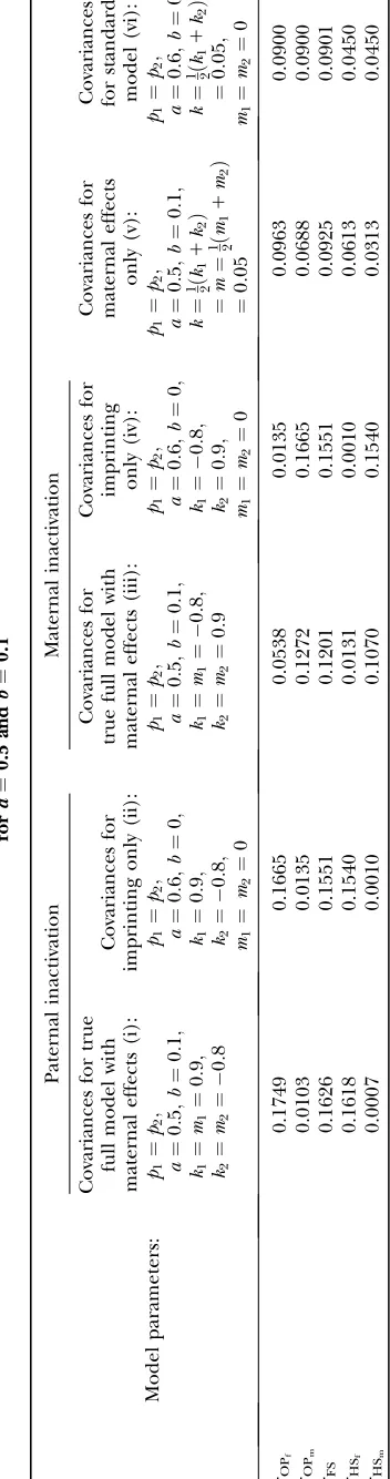
We may examine the covariances between relatives derived in approach 1 and can see that both imprinting and maternal effects add extra terms. Ignoring imprint-ing and maternal effects may over- or underestimate true covariances. For example, Tables 9 and 10 calculate parent–offspring, full-sib, and half-sib covariances for six models: (i) a full model incorporating paternal in-activation and maternal effects, (ii) a model including paternal inactivation only, (iii) a full model incorporat-ing maternal inactivation and maternal effects, (iv) a model including maternal inactivation only, (v) a model including maternal effects only, and (vi) a standard two-allele model without imprinting or maternal effects. Assuming that both maternal effects and imprinting are influencing this trait, we have calculated the true ex-pected population covariances under both paternal inacti-vation (model i) and maternal inactiinacti-vation (model iii). Table 9 calculates these covariances fora¼0.5 andb¼

be calculated separately for maternal and paternal inactivation as do models i–iv.

A number of conclusions are apparent from exami-nation of Tables 9 and 10. For paternal inactivation and maternal effects in Table 9 (model i) we can see that

sOPf.sFS.sHSf.sOPm.sHSm. Note also that models ii, v, and vi underestimate the true values for sOPf;

sFS;andsHSf while overestimating values for sOPm andsHSm. Model ii retains the relative ordering of co-variances while model v incorrectly rankssOPm ahead of

s_HSf. Estimates for model vi do not compare well to the true values calculated in model i.

For maternal inactivation with maternal effects in Table 9 (model iii) the relative ordering of covariances is

sOPm.sFS.sHSm.sOPf.sHSf. Model iv overestimates while models v and vi underestimate sOPm;sFS;and

sHSm. All three models iv, v, and vi underestimate

sOPfandsHSf. Model iv retains the relative ranking of covariances from the true model iii, although estimates from and order ranking of models v and vi do not compare well to model iii.

Quite different observations are apparent when ex-amining Table 10, for covariances calculated assum-ing maternal effects and own genotype effects have equal impact on genotypic values of offspring. For paternal inactivation and maternal effects (model i), the relative ordering of covariances is nows_FS.s_HSf.

s_OPf.s_OPm.s_HSm. Once again models ii, v, and vi underestimatesOPf;sFS;andsHSf while overestimating

sOPmandsHSm. In contrast to Table 9, however, model v now appears to best estimate relative sizes and ordering of covariances.

For maternal inactivation in Table 10, an even more surprising result is apparent. Because maternal alleles are almost completely inactivated, we would expect

sOPmandsHSm to rank highly, as they did in Table 9. However our covariances between relatives now follow

sFS.sOPf.sHSf.sOPm.sHSm. There is no consistent pattern of over- or underestimation of covariances when comparing to the alternative models iv, v, and vi. As was the case for paternal inactivation discussed above, model v (maternal effects alone) appears to best mimic the covariance structure. Despite maternal effects and offspring own genotype having equally weighted con-tributions to offspring genotypic value (a¼b¼0.3), it is apparent from this example that maternal genotype effects, and not imprinting effects, have greatest impact on the covariances between relatives. Further, simula-tion results (data not shown) suggest that maternal effects can outweigh imprinting effects even whenb>a, especially when the difference between reciprocal het-erozygotes is not large. For example, if a¼0:4;b ¼

0:2;k1 ¼m1¼ 0:1;andk2 ¼m2 ¼0:2 (higher pater-nal than materpater-nal expression of alleles, plus materpater-nal effects), thens_OPf ¼0:0920 ands_OPm ¼0:0575.

We are likely to have population estimates for covar-iances between relatives. It is pertinent to assess whether

T

ABLE

9

Comparison

of

co

va

riance

predic

ti

o

n

s

u

si

ng

inco

mpletely

specified

models

o

f

imprin

ti

ng

only

,

mater

n

al

ef

fects

only

,

and

n

o

imprinting

o

r

m

at

er

nal

e

ff

e

ct

s,

fo

r

a

¼

0.

5

and

b

¼

0.1

Paternal

inactivation

Maternal

inactivation

Covariances

for

true

full

model

with

maternal

effects

(i):

Covariances

for

imprinting

only

(ii):

Covariances

for

true

full

model

with

maternal

effects

(iii):

Covariances

for

imprinting only

(iv):

Covariances

for

maternal

effects

only

(v):

Covariances for

standard

model

(vi):

Model

parameters:

p1

¼

p2

;

a

¼

0

:

5

;

b

¼

0

:

1

;

k1

¼

m1

¼

0

:

9

;

k2

¼

m2

¼

0

:

8

p1

¼

p2

;

a

¼

0

:

6

;

b

¼

0

;

k1

¼

0

:

9

;

k2

¼

0

:

8

;

m1

¼

m2

¼

0

p1

¼

p2

;

a

¼

0

:

5

;

b

¼

0

:

1

;

k1

¼

m1

¼

0

:

8

;

k2

¼

m2

¼

0

:

9

p1

¼

p2

;

a

¼

0

:

6

;

b

¼

0

;

k1

¼

0

:

8

;

k2

¼

0

:

9

;

m1

¼

m2

¼

0

p1

¼

p2

;

a

¼

0

:

5

;

b

¼

0

:

1

;

k

¼

1ðk2

1

1

k2

Þ

¼

m

¼

1ðm2

1

1

m2

Þ

¼

0

:

05

p1

¼

p2

;

a

¼

0

:

6

;

b

¼

0

;

k

¼

1ðk2

1

1

k2

Þ

¼

0

:

05

;

m1

¼

m2

¼

0

sOP

f

0.1749

0.1665

0.0538

0.0135

0.0963

0.0900

sOP

m

0.0103

0.0135

0.1272

0.1665

0.0688

0.0900

sFS

0.1626

0.1551

0.1201

0.1551

0.0925

0.0901

sHS

f

0.1618

0.1540

0.0131

0.0010

0.0613

0.0450

sHS

m

0.0007

0.0010

0.1070

0.1540

0.0313

we can estimate values fora,b,k1,k2,m1, andm2given these covariances. Let us take the parameters and calculated covariances from model i in Table 9 (pater-nal inactivation with mater(pater-nal effects). We assume

p1¼p2¼0:5, a;b.0, and that heterozygotes are re-strained to fall within the range of the homozy-gotes (that is, k1;k2;m1;m2 2 ½1;1). We also set

k1¼m1andk2 ¼m2, so that mother and offspring notypes act in the same way on overall offspring ge-notypic value. For example, anA2A1offspring with an

A2A1 mother will have a contribution to overall off-spring genotypic value ofa(11k1) from its own geno-type and a contribution ofb(11k1) from its mother’s genotype.

We endeavor to retrieve known parameter values for

a,b,k1(¼m1) andk2(¼m2) by setting the calculated values for covariances between relatives equal to their mathematical expressions and solving simultaneously. We have five equations and four unknowns, but because all five covariances involve quadratic terms in the pa-rameters we are trying to estimate (a,b,k1, andk2) they do not have unique solutions for the given calculated covariances. However, applying our range constraints gives two solutions,

a¼0:5;b¼0:1;k1¼0:9;k2¼ 0:8;m1¼0:9;andm2¼ 0:8

(our original values) and

a¼0:5;b¼0:1;k1¼ 0:8;k2¼0:9;m1¼ 0:8;andm2¼0:9

(Table 11, full model, row 2). Values ofaandbare the same for the two solutions, maintaining the relative contribution of maternal effects to the range of geno-typic values. However, it is interesting to note that the two solutions exchange values fork1andk2(andm1and

m2) as a consequence of our assumption of equal allele frequencies in the population. As seen in Table 9, if there are large differences between predicted values for reciprocal heterozygotes and between estimates for a

and b, a much larger population value for sOPf com-pared to s_OPm is indicative of paternal inactivation. Therefore we are able to conclude that the first solution is the true solution for the population. However, as was clear from Table 10, without large differences betweena

andbandk1andk2, it may not be possible to determine which set of values for a, b, k1, andk2 is true for the population. This highlights an important theoretical restriction: it may not be possible to differentiate ma-ternal effects from imprinting using observed popula-tion covariances—even when assumppopula-tions are made about population allele frequencies and values and ranges for

k1,k2,m1, andm2.

We may also assess how incorrectly specifying the model affects our estimates fora,b,k1,k2,m1, andm2. We again take the known values for covariances from model i in Table 9 and use our expressions for covariances between relatives as derived in approach 1 under the

T

ABLE

10

Comparison

of

covariance

predictions

using

incompletely

specified

models

of

imprinting

only

,

mater

nal

ef

fects

only

,

and

no

imprinting

or

mater

nal

e

ffects,

for

a

¼

0.3

and

b

¼

0.3

Paternal

inactivation

Maternal

inactivation

Covariances

for

true

full

model

with

maternal

effects

(i):

Covariances

for

imprinting only

(ii):

Covariances

for

true

full

model

with

maternal

effects

(iii):

Covariances

for

imprinting only

(iv):

Covariances

for

maternal

effects

only

(v):

Covariances

for

standard

model

(vi):

Model

parameters:

p1

¼

p2

;

a

¼

0

:

3

;

b

¼

0

:

3

;

k1

¼

m1

¼

0

:

9

;

k2

¼

m2

¼

0

:

8

p1

¼

p2

;

a

¼

0

:

6

;

b

¼

0

;

k1

¼

0

:

9

;

k2

¼

0

:

8

;

m1

¼

m2

¼

0

p1

¼

p2

;

a

¼

0

:

3

;

b

¼

0

:

3

;

k1

¼

m1

¼

0

:

8

;

k2

¼

m2

¼

0

:

9

p1

¼

p2

;

a

¼

0

:

6

;

b

¼

0

;

k1

¼

0

:

8

;

k2

¼

0

:

9

;

m1

¼

m2

¼

0

p1

¼

p2

;

a

¼

0

:

3

;

b

¼

0

:

3

;

k

¼

1ðk2

1

1

k2

Þ

¼

m

¼

1ðm2

1

1

m2

Þ

¼

0

:

05

p1

¼

p2

;

a

¼

0

:

6

;

b

¼

0

;

k

¼

1ðk2

1

1

k2

Þ

¼

0

:

05

;

m1

¼

m2

¼

0

sOP

f

0.1816

0.1665

0.0860

0.0135

0.1013

0.0900

sOP

m

0.0051

0.0135

0.0624

0.1665

0.0338

0.0900

sFS

0.1996

0.1551

0.1231

0.1551

0.1126

0.0901

sHS

f

0.1993

0.1540

0.0846

0.0010

0.1013

0.0450

sHS

m

0.0003

0.0010

0.0385

0.1540

0.0113

three reduced models: no imprinting (maternal effects only), no maternal effects (imprinting only), and no maternal effects or imprinting. By setting the reduced expressions for covariances equal to the true values and solving, we find that in many cases we are unable to recover consistent solutions for the reduced models (Table 11). We define consistent solutions as solutions satisfying our constraints on a;b;k1;k2;m1; andm2ðor

kandmÞ. The lack of consistent solutions for the re-duced models is an indication that the models are in-complete and that additional genetic factors are acting that have not been specified.

Examining columns 1 and 3 in Table 11, we can see that the assumptions of the three reduced models affect the restraints that are placed on our parameters: for example, under a reduced model of maternal effects only,k1¼k2¼kandm1¼m2¼mfor all covariances, and we now have a condition thatk;m2 ½1;1. Note that this also affects the number of parameters we are solving for in each of the reduced models, and hence to find a solution we must solve for subsets of covariances, rather than using all five true covariance values (Table 11, column 2). Interestingly, a consistent solution pair was found for all three reduced models using a subset of full-sib and half-sib covariances: for imprinting only,

fa;k1;k2g ¼ f0:6064;0:8351;0:9175g

orf0:6064;0:9176; 0:8351g;

for maternal effects only,

fa;b;kð¼mÞg ¼ f0:0750;0:5892;0:3333g

orf0:0750;0:5892;0:3333g;

and for no maternal effects or imprinting,

fa;kg ¼ f0:8063;0:0310gorf0:8063;0:0310g:

As we also saw in the two solutions to the full model, for the imprinting-only modelk1(andk2) reversed sign between two solution sets, effectively reversing the pre-diction from maternal to paternal inactivation of alleles. A similar result was seen in the no imprinting, no maternal effects model where the A1 allele changed from recessiveðk¼ 0:0310Þto dominantðk¼0:0310Þ

in two solutions to the same simultaneous equations. In addition, it is interesting to note that the maternal-effects model estimated a much larger maternal effect (b) than the true value, while the other two models overestimated own genotype effect (a). This in general was also true of consistent estimates for a and b con-tained within inconsistent solution sets for these three reduced models. As would be expected, therefore, not including maternal effects in the model will overesti-mate the contribution from an offspring’s own geno-type to genotypic values and covariances.

Many of the inconsistent solutions included imagi-nary numbers. Examining column 5 of Table 11, we see

a large range in estimates for parameters contained within these inconsistent solutions. Perhaps not surpris-ingly, this result suggests that consistent parameter val-ues contained within inconsistent solution sets should not be used to infer population parameters. It can be noted from this example that inconsistent solutions, solutions containing imaginary numbers, and even the presence of more than one solution should highlight to the researcher that an incorrect model has been employed.

From Tables 9–11 we have seen that misspecification of the model can have huge implications on parameter and covariance estimation, and it is clearly important to allow for imprinting and maternal effects when estimat-ing parameters and covariances. Nevertheless, research-ers should be aware that even in using a complete model and known covariances between a range of relatives, they may not be able to differentiate between maternal and paternal expression if maternal genotype is having a significant effect and differences between reciprocal heterozygotes are small.

The authors thank B. L. Harris and K. G. Dodds for discussion and two anonymous reviewers for their very helpful suggestions to improve the manuscript. This work was supported by the Livestock Improve-ment Corporation and the Allan Wilson Centre for Molecular Ecology and Evolution. A.W.S. was the recipient of a Bright Future Enterprise Doctoral Scholarship from the New Zealand Foundation for Research, Science, and Technology and the Tertiary Education Commission and a Postgraduate Publishing Award from the University of Otago Re-search Committee.

LITERATURE CITED

Bartolomei_{, M. S., and S. M. T}ilghman_{, 1997 Genomic imprinting}

in mammals. Annu. Rev. Genet.31:493–525.

De_Chiara_{, T. M., E. J. R}obertson_{and A. E}fstratiadis_{, 1991 Parental}

imprinting of the mouse insulin-like growth factor II gene. Cell64:

849–859.

Falconer, D. S., and T. F. C. Mackay, 1996 Introduction to

Quantita-tive Genetics, Ed. 4. Longman, Harlow, Essex, UK.

Huck_{, U. W., J. B. L}abov_{and R. D. L}isk_{, 1987 Food-restricting first}

generation juvenile female hamsters (Mesocricetus auratus) affects sex ratio and growth of third generation offspring. Biol. Reprod.

37:612–617.

Kempthorne_{, O., 1957 An Introduction to Genetic Statistics. John Wiley}

& Sons, New York.

Lynch_{, M., and B. W}alsh_{, 1998 Genetics and Analysis of Quantitative}

Traits. Sinauer Associates, Sunderland, MA.

Moore, A. J., J. B. Wolfand E. D. Brodie, III, 1998 The influence of

direct and indirect genetic effects on the evolution of behavior: social and sexual selection meet maternal effects, pp. 22–41 in

Maternal Effects as Adaptations, edited by T. A. Mousseau _and

C. W. Fox. Oxford University Press, New York.

Morison_{, I. M., J. P. R}amsay_{and H. G. S}pencer_{, 2005 A census of}

mammalian imprinting. Trends Genet.21:457–465.

Naumova_{, A. K., and S. C}roteau_{, 2004 Mechanisms of}

epi-genetic variation: polymorphic imprinting. Curr. Genomics 5:

417–429.

O’Neill_{, M. J., R. S. I}ngram_{, P. B. V}rana_{and S. M. T}ilghman_,

2000 Allelic expression of IGF2 in marsupials and birds. Dev. Genes Evol.210:18–20.

Sandovici, I., M. Leppert, P. R. Hawk, A. Suarez, Y. Linareset al.,

Sandovici, I., S. Kassovska-Bratinova, J. C. Loredo-Osti,

M. Leppert_{, A. S}uarez _{et al., 2005 Interindividual variability}

and parent of origin DNA methylation differences at specific hu-manAluelements. Hum. Mol. Genet.14:2135–2143.

Shaw, R. G., and D. L. Byers, 1998 Genetics of maternal and paternal

effects, pp. 97–111 inMaternal Effects as Adaptations, edited by T. A. Mousseauand C. W. Fox. Oxford University Press, New York.

Spencer, H. G., 2002 The correlation between relatives on the

sup-position of genomic imprinting. Genetics161:411–417.

Wade, M. J., 1998 The evolutionary genetics of maternal effects, pp.

5–21 inMaternal Effects as Adaptations, edited by T. A. Mousseau

and C. W. Fox. Oxford University Press, New York.

Wolf_{, J. B., T. T. V}aughn_{, L. S. P}letscher_{and J. M. C}heverud_,

2002 Contribution of maternal effect QTL to genetic architec-ture of early growth in mice. Heredity89:300–310.