Disentangling Linkage Disequilibrium and Linkage From Dense Single-Nucleotide Polymorphism Trio Data

DOI: 10.1534/genetics.105.047431

Disentangling Linkage Disequilibrium and Linkage From Dense

Single-Nucleotide Polymorphism Trio Data

Geraldine M. Clarke

1

_{and Lon R. Cardon}

Wellcome Trust Centre for Human Genetics, Oxford University, Oxford OX3 7BN, United Kingdom Manuscript received June 29, 2005

Accepted for publication August 2, 2005

ABSTRACT

Parent-offspring trios are widely collected for disease gene-mapping studies and are being extensively genotyped as part of the International HapMap Project. With dense maps of markers on trios, the effects of LD and linkage can be separated, allowing estimation of recombination rates in a model-free setting. Here we define a model-free multipoint method on the basis of dense sequence polymorphism data from parent-offspring trios to estimate intermarker recombination rates. We use simulations to show that this method has up to 92% power to detect recombination hotspots of intensity 25 times background over a region of size 10 kb typed at density 1 marker per 2.5 kb and almost 100% power to detect large hotspots of intensity.125 times background over regions of size 10 kb typed with just 1 marker per 5 kb (a¼ 0.05). We found strong agreement at megabase scales between estimates from our method applied to HapMap trio data and estimates from the genetic map. At finer scales, using Centre d’Etude du Poly-morphisme Humain (CEPH) pedigree data across a 10-Mb region of chromosome 20, a comparison of population recombination rate estimates obtained from our method with estimates obtained using a coalescent-based approximate-likelihood method implemented in PHASE 2.0 shows detection of the same coldspots and most hotspots: The Spearman rank correlation between the estimates from our method and those from PHASE is 0.58 (p,2.216_).

L

INKAGE disequilibrium (LD) refers to the pres-ence of nonrandom association among two or more alleles at distinct loci. The degree of LD between alleles is determined by an evolutionary process com-bining the effects of natural selection, mutation, ge-netic drift, and population admixture. Appreciable LD is likely to be present only between two loci that are tightly linked. For this reason, attempts have been made to use the magnitude of LD between two loci to obtain estimates of recombination fractions between loci,e.g., Serreet al.(1990). Transmission of haplotypes

from parents to offspring is dependent on both LD and linkage (Spielmanet al.1993). Specifically, the extent

of LD between two distinct loci decays exponentially at a rate proportional to the recombination fractionc

between the loci: If the disequilibrium between the two loci is D0 at time 0, then after k generations the

disequilibrium will be

Dk¼ ð1cÞkD0: ð1Þ

Hence, if either the time span or the recombination rate is known, then, under simplifying assumptions that ignore the ongoing stochastic effect of the evolutionary

process, the other parameter can be estimated from the coefficients of LD (Lander and Botstein 1986). In

practice, such estimates are problematic because the sampling variance of LD tends to be very large due to the evolutionary sampling (Hilland Weir1994), resulting

in large standard errors in the estimate ofc. Motivated by the extensive genotyping on familial trios (mother, father, and offspring) in the International HapMap Project (InternationalHapMapConsortium2003),

as well as by the availability of large trio samples in several disease cohorts, we construct a simple, robust, approach to disentangling the effects of LD and linkage in the transmission of data from parent to offspring. Our method relates the genetic variation in a popula-tion sample over one generapopula-tion to the underlying recombination rate and uses a multipoint approach to reduce the standard error normally associated with LD-based methods. We make only the usual assumptions of genetic equilibrium required for establishment of Hardy-Weinberg equilibrium. Specifically, we make the following explicit assumptions: infinite population size, discrete generations, random mating, no selection, no migration, no mutation, and no difference across sexes in parental genotype frequencies. In this sense, our method can be described as model-free. The trans-mission data between multiple pairs of overlapping densely spaced markers is combined to reduce var-iance and produce accurate estimates of recombination

1_{Corresponding author:Wellcome Trust Centre for Human Genetics,}

Oxford University, Roosevelt Dr., Oxford OX3 7BN, United Kingdom. E-mail: [email protected]

rates between adjacent markers. Our method generates short-range smoothness in recombination rates over the region of the chromosome spanned by overlapping markers and allows for rate estimation on various scales limited only by the density of the markers used.

More sophisticated methods applying models to ac-count for stochastic effects have been developed and used successfully for the fine mapping of disease genes using allelic associations in isolated populations, for ex-ample, those in Hastbackaet al.(1992), Kaplanand

Weir (1995), Kaplan et al. (1995), and Devlin et al.

(1996). Also, many coalescent model-based methods exist for the estimation of recombination rates from patterns of sequence variation in population genetic data. Methods include moment-based estimators (Wall

2000) and full-likelihood (Griffiths and Marjoram

1996; Kuhner _{et al.} 2000; Nielson 2000; Fearnhead

and Donnelly 2001) and approximate-likelihood

ap-proaches (Hudson 2001; Fearnhead and Donnelly

2002; Mcvean et al. 2002; Li and Stephens 2003).

Methods are further described in Stumphand Mcvean

(2003).

We define a hotspot of intensitysto be a region of length 10 kb where crossovers occur a frequency of more thanstimes that in the surrounding region. We use simulations to show that, using 200 trio families, our method can reliably detect recombination hotspots of intensity 10 across a region typed with 20 markers at a density of 1 marker per 2.5 kb (P,0.025). Hotspots of an intensity.25 can be detected by typing as few as 5 markers at a density of 1 marker per 2.5 kb (P,0.001). We show that the number of markers required to achieve a given accuracy decreases with marker density. Results suggest that this method is able to detect fine-scale variation in recombination rate according to the density of typed markers: That is, the more dense the marker spacing is, the more fine scale the variation that can be detected. To validate our approach, we estimated recombination rates using HapMap Centre d’Etude du Polymorphisme Humain (CEPH) trio data from various chromosomes and compared averages over a megabase scale to estimates from the genetic map (Konget al.2002).

At a finer scale, we compared recombination rate esti-mates in European (CEPH) populations between adja-cent SNPs on a 10-Mb region of chromosome 20 made using our model-free method to independent estimates made from a coalescent model-based approximate-likelihood approach implemented in the program PHASE 2.0 (Stephens et al. 2001; Stephens and Donnelly

2003). These independent estimates are described in detail in Evansand Cardon(2005).

METHODS

We assume that we have phase-known genotype data from N familial trios at L densely spaced, ordered,

biallelic markers. Seediscussionfor comments on how

to handle phase-unknown genotype data. Markers are labeled 1,. . ., L. We summarize the data at all pairs of markers up to a given distance apart (e.g., all pairs of markers up to w markers apart, w, L) as counts of observed haplotypes in both parental and offspring generations. The method can be summarized in three stages as follows:

1. For all pairs of markers, we first estimate the prob-ability of observing each haplotype in the parental population. This provides an estimate of LD in the parental generation.

2. For each pair of markers, we write down the likeli-hood of transmitting the observed offspring haplo-type counts conditional on the LD in the parental generation, that is, assuming the LD in the parental generation is a known parameter. The likelihood of transmitted haplotype counts at each pair of markers is a function of the recombination fraction between the markers. The recombination fraction is defined as the probability that a transmitted haplotype con-stitutes a new combination of alleles different from that of either parental haplotype. Maximum-likelihood estimates (MLEs) of the recombination fraction are then obtained, independently, at all pairs of markers.

3. Finally, for any given pair of adjacent markers, all estimates from marker pairs that overlap the adjacent pair, up to a given distance apart, are scaled accord-ing to the interval spanned by the pair of markers relative to the interval spanned by the adjacent mark-ers under consideration. Each scaled estimate repre-sents a new estimate of the recombination fraction between the adjacent pair of markers. The original estimate between each pair of markers and all new estimates are then averaged (weighted by variance) to form a final, new estimate of the recombina-tion fracrecombina-tion between each pair of adjacent markers. These steps are now described in greater detail.

Step 1—determine LD in the parental generation:

Consider any two biallelic markers with alleles arbitrarily labeled A and a at the first locus and B and b at the second locus. Let cbe the recombination fraction be-tween the markers. We assume that haplotypes are available or have been estimated from a sample of N

parent-offspring trios. The four possible haplotypes are

ab,aB,Ab, and ABand the observed number of these haplotypes in the parental generation is denoted bym¼

(mab,maB,mAb,mAB), withmab1maB1mAb1mAB¼4N.

The likelihood of a specific sample configuration is

LðmÞ ¼ ð4NÞ! mab!maB!mAb!mAB!

pmab

ab pmaBaBpAbmAbpaBmAB; ð2Þ

wherepab,paB,pAb, andpABare the frequencies of

generation. The MLE ofpabismab=4N and is denoted by ^

pab and likewise for paB, pAb, andpAB. Let estimates of

major allele frequencies at each locus be given by

^

pA¼^pAb1^pABand^pB¼^pAB1^paB. Using the standard

notation for an LD coefficient, we let

D¼pABpApB

denote the LD in the parental generation. Let

^

D¼_p^_AB^_pAp^_B

denote the MLE of LD in the parental generation.

Step 2—infer recombination fraction c between

markers: Letp9ab be the frequency of haplotype abin

the offspring generation. Then, by conditioning on all possible parental haplotype combinations from which anabhaplotype can be transmitted, it is easy to see that

p9ab¼pab2 1pabpaB1pabpAb1pabpABð1cÞ1paBpAbc ¼pabðpab1paB1pAb1pABÞ cðpabpABpaBpAbÞ ¼pabcðpAB ðpAb1pABÞðpAB1paBÞÞ

¼pabDc: ð3Þ

Similarly, it is easy to show that the frequencies of haplotypesaB,Ab, andABin the offspring generation are, respectively,

p9aB¼paB1Dc;

p9_Ab¼pAb1Dc

and

p9AB ¼pABDc:

Let the observed number of haplotypes in the off-spring generation be denoted by

n¼ ðnab;naB;nAb;nABÞ;

wherenab1naB1nAb1nAB¼2N. Using MLEs of

par-ental haplotype probabilities, the likelihood at c for a specific sample configuration of offspring haplotypes is therefore given by

LðcÞ ¼ ð^_pabDc^ _Þnab_ð^_p

aB1Dc^ ÞnaBð^pAb1Dc^ ÞnAbð^pABDc^ ÞnAB:

ð4Þ

MLEs^cofcare obtained by selecting the value ofcthat maximizes Equation 4. The information I(c) for c is defined as minus the second derivative of Equation 4:

IðcÞ ¼_D^2 nab ð^pabDcÞ^ 2

1 naB

ð^paB1DcÞ^ 2

1 nAb

ðp^Ab1DcÞ^ 2

1 nAB

ð^pABDcÞ^ 2

:

ð5Þ

I(c) evaluated at^c is the observed information and is inversely proportional to the asymptotic variance of^c. LetVð^cÞdenote the variance of estimate^c. Observe that whenD^ is small, as would be the case in recombination

hotspots, the likelihood has less dependence on the exact value of c and MLEs will have large variance. Conversely, whenD^ is large, estimates ofcwill be more precise with small variance.

Step 3—use multiple closely linked flanking markers to refine estimate ofc: Letdi,jbe the distance, in base

pairs, between any two markersiandj. Letci,jrepresent

the recombination fraction between markers i and j

and let^ci;jbe the MLE ofci,jobtained using the method

described above. Individual estimates of ^ci;j can be

highly variable. To refine our estimate ^ci;i11 between

adjacent markersiandi11, we combine estimates^cj;k

obtained at multiple pairs of markers jand kup tow

markers away from markers i and i1 1, i.e., pairs of markers inS:¼ f(j,k) : max(0,i11w)#j,k#min (i1w,L)g. These represent all the markers that overlap markersiandi11 and are withinwmarkers of them and are referred to as theflanking markers. We assume that the rate at which recombination occurs remains constant over the region of the chromosome spanned by the flanking markers. Since recombination fractions are approximately additive over short distances and our markers are densely spaced, we assume that the inter-marker recombination fractions estimated between pairs of flanking markers are scaled estimates of the intermarker recombination fraction between markersi

andi11. Specifically, let

^c_i;iðj;k1Þ1¼

di;i11

dj;k

^cj;k

be an estimate ofci,i11on the basis of data from thefj,kg

interval. Then the variance of^c_ið;ji1;k1Þis

V ^c_ið;j;ki1Þ1

¼ di;i11 dj;k

2

Vð^cj;kÞ:

We form a new estimate^^ci;i11 of ci,i11, by taking the

weighted average of all estimatesc^_ið;ij;1kÞ1, (j,k)2S.

Spe-cifically, let

^ ^

ci;i11¼

P

SWi;j;k^c ðj;kÞ i;i11

P

SWi;j;k

; ð6Þ

where

Wi;j;k¼

1

V ^c_i;iðj1;kÞ1

is the weight given to the estimated intermarker re-combination fraction between markersiandi11 made on the basis of information from markersjandk. Figure 1 illustrates these steps in more detail.

If estimates are independent andNlarge then^^ci;i11is

approximately distributed as a normal random variable with meanci,i11and varianceVðc^^i;i11Þ(Edwards1992),

Vð^^ci;i11Þ ¼

1

ðP_SWi;j;kÞ2

X

S

ðWi;j;kÞ2V ^c ðj;kÞ i;i11

¼P 1

SWi;j;k

:

ð7Þ

However, estimates c^ið;ij1;kÞ1, (j, k) 2 S, are, in fact,

dependent. For the analysis presented here, we violate the assumption of independence and use the formula given in Equation 7 to get rough approximations of normal confidence intervals. Refer to thediscussion

for alternative possibilities for computing the variance.

Simulations:To test the accuracy of our method for

estimating recombination fractions between loci we used the program fin (software available on request from G. A. T. Mcvean, [email protected]) to gen-erate SNP genotype data simulated from a standard coalescent neutral model of genetic variation. The basic simulation involved 400 sequences of 400 SNPs with an overall population recombination rate,r¼4Ner¼400,

whereNeis the effective population size andris the per

generation recombination rate, that is, the probability of a crossover per generation across the 1-Mb region. For an effective population size ofNe¼10,000, thenr¼

0.01 over the 1-Mb region, equivalent to a genetic dis-tance of 1 cM/Mb, which is approximately the rate seen in human data derived from observed crossovers in pedigrees (Konget al. 2002). Average SNP spacing is 1

SNP perd¼2.5 kb. The population recombination rate was set at a constant background value over the sim-ulated region but increased to sizes¼10 times the back-ground rate at three evenly spaced intervals of length 10 kb. Hence, for this simulation, there were 385 mark-ers with intermarker recombination rate value 0.748; the remaining 15 markers were simulated to be in three hotspots of 5 markers with intermarker recombination rate value 7.48. Thus, in total, the overall population recombination rate isr¼153 7.48138530.748¼

400, as required, and crossovers between markers in the hotspot were simulated to occur 10 times more fre-quently than those in the surrounding sequence. Sam-ples were then randomly mated using the program tdtsim (software available on request from A. Morris, [email protected]) to produce 200 offspring sam-ples with zero recombination. We show that recombi-nation in current generation meioses does not have a significant impact on estimated recombination rates using our method. Simulations were repeated as de-scribed for hotspot intensitiess¼1, 25, 125, and 625. Obviously, simulations withs¼1 have uniform recom-bination rate across the region,i.e., no hotspots, and are used for comparison.

Intermarker recombination fraction estimates were estimated for each simulation and converted to genetic distances in centimorgans per megabase as follows.cis multiplied by 100, to convert to centimorgans, and then divided by the intermarker interval length in mega-bases, to convert to centimorgans per megabase. To ensure a mean value of 1 cM/Mb across the region, estimates are scaled by dividing by the estimated total genetic distance across the 1-Mb region. Since recom-bination fractions are ,0.01, conversion to genetic distances requires no mapping function.

RESULTS

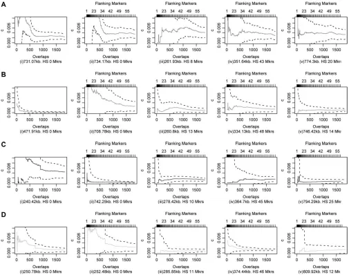
Figure 2 shows intermarker recombination fraction estimates for randomly selected markers according to the number of pairs of overlapping markers used to refine each estimate. Observe that estimates have large confidence intervals when using information from just the adjacent pair (equivalent to 1 overlap or 1 flanking marker) but the variance reduces, and estimates settle to specific values, as the number of flanking markers used to refine the estimate increases. Clearly, information from a single pair of markers does not provide enough information to accurately estimate intermarker recom-bination fractions in this way. The strength of our

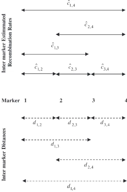
Figure_{1.—Consider four markers with intermarker}

distan-ces noted. MLEs^c1;4,^c2;4,^c1;3,^c1;2,^c2;3, and^c3;4 of the

inter-marker recombination fractions are made for each pair of markers. New estimates for the interval between markers 2 and 3 are made from markers 1 and 3, markers 2 and 4, and markers 1 and 4 as ^c2ð1;3;3Þ¼ðd2;3=d1;3Þ^c1;3, ^c

ð2;4Þ

2;3 ¼ðd2;3=d2;4Þ^c2;4, and ^cð21;3;4Þ¼ðd2;3=d1;4Þ^c1;4, respectively. A weighted average of these

new estimates provides a final refined estimate,^^c2;3, of the

method comes from combining estimates at pairs of overlapping markers. The number of flanking markers to use will depend on the marker density, the scale of recombination to be detected, and the number of avail-able trios. Appropriate selection ofwis discussed in the

discussion.

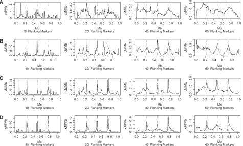
Figure 3 shows intermarker recombination rates, in centimorgans per megabase, from simulations de-scribed for Figure 2. Each row corresponds to a different true hotspot intensity, s ¼ 10, 25, 125, and 625, and illustrates results at 10, 20, 40, and 60 flanking markers. Estimates plotted in centimorgans per megabase appear smoothed because: (1) The intermarker recombination

fraction estimates depend on the intermarker distances and (2) the method assumes constancy of recombina-tion rate over the distance covered by the flanking markers that are used to refine each intermarker esti-mate. Plots indicate that hotspots start to appear at as few as 10 flanking markers; large hotspots of 625 times background are well defined at this point (Figure 3D). Clearly, the larger the hotspot intensity is, the easier it is to detect and using more markers increases the ability to detect hotspots. The last column of Figure 3 indicates that when 60 flanking markers are used to refine the intermarker recombination rate estimates, the method can successfully detect hotspots of each intensity. Note

Figure2.—Estimates of intermarker recombination fractions for randomly selected markers according to the number of

that the presence of peaks at locations other than model hotspots may still be valid since our data are randomly generated.

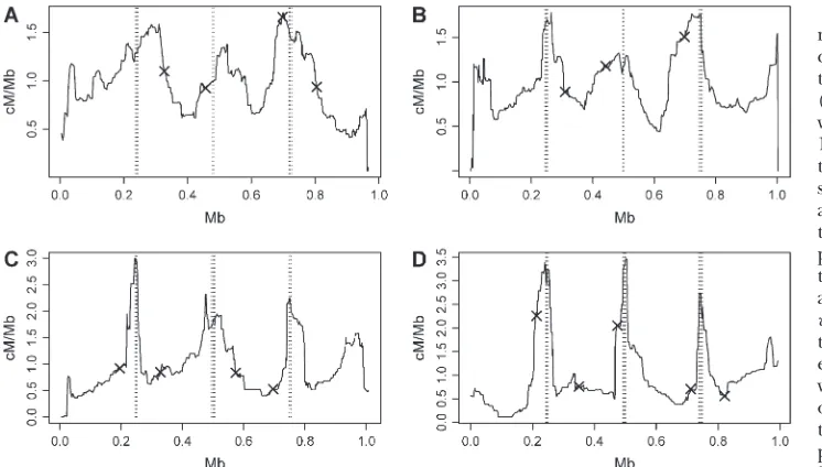
Figure 4 shows results similar to those given in Figure 3 but where the current generation of offspring was cre-ated, allowing an expected value of four recombina-tions in their parental meioses per 1 Mb of simulated sequence. The solid crosses indicate the site of a re-combination that occurred in the current generation. Clearly, recombination in the current generation does not have a significant impact on our estimates of popu-lation recombination rates. Our method appears to capture historical recombination rate information.

Consistency: To assess more formally whether our

method was able to consistently detect hotspots and to analyze the impact of marker density, simulations were repeated 1000 times for each hotspot intensity,s¼1, 10, 25, 125, 625 times background and for new marker densities 1 marker per 2 and 5 kb. We refer to a set of 1000 simulations as a simulation group. For each sim-ulation we used our method to estimate intermarker recombination fractions for various numbers of flank-ing markers. For each set of estimated intermarker

recombination fractions, we estimated hotspot intensity. Estimated hotspot intensity is calculated as the esti-mated mean genetic distance (centimorgans per mega-base) at the simulated hotspot sites divided by that at the simulated nonhotspot sites.

Figure 5 shows the estimated mean hotspot inten-sity by flanking markers for each simulation group at marker density 1 marker per 2.5 kb. Dotted lines indi-cate 95% bootstrap percentile confidence intervals (Efronand Tibshirani1993). For any value of flanking

markers used, Figure 5 shows, as indicated in Figure 2, that estimates of hotspot intensity are relatively correct although they are not linearly related;i.e., the line for 625 times background is still higher than the line for 125 times background but not 5 times greater. Clearly the method can detect hotspots of different intensity but problems of scale are related to the way that the method utilizes nearby markers to refine estimates. The effect of refining estimates over multiple pairs of markers also smoothes them.

To formally test whether a hotspot has been detected in simulations from groups where s . 1, we consider a null hypothesis that the simulation true hotspot

Figure3.—Estimates of intermarker recombination rates, in centimorgans per megabase, plotted at marker midpoint location

intensity is 1. For a type I error rate of 0.05, we use the 95th percentile of estimated hotspot intensity value from simulation groups wheres¼1 as critical values and accept the alternative hypothesis that a simulation true hotspot intensity is.1 if the estimated hotspot intensity from that simulation is greater than the corresponding critical value. We define the power of our test in a given simulation group to be the proportion of simulations

from that group with estimated hotspot intensities greater than the corresponding critical value.

Figure 6 shows the power of our test to detect a hot-spot for each simulated true hothot-spot intensity,s¼10, 25, 125, and 625 times background, and marker density 1 marker per 2, 2.5, and 5 kb, according to the number of flanking markers. Power appears to increase with number of flanking markers used, up to a point: Graphs

Figure 4.—Estimates of

inter-marker recombination rates, in centimorgans per megabase, plot-ted at marker midpoint location (in megabases) for simulations with true hotspot intensities (A) 10, (B) 25, (C) 125, and (D) 625 times background and where off-spring have been generated with a mean population recombina-tion rate of four recombinarecombina-tions per megabase per generation over the simulated sequence. Results are forw¼60 flanking markers: wflanking markers means that in-termarker recombination fraction estimates from all marker pairs withinwmarkers of a given pair of markers were used to refine the estimate at that given marker pair. Results are for simulations in 200 trios of 400 SNP markers at a mean spacing of 2.5 kb over a 1-Mb region with three evenly spaced hotspots. The solid vertical dashed lines indicate the true locations of these hotspots. The solid crosses indicate the true locations of recombinations occurring in offspring meioses. Refer to the text for a discussion of how intermarker recombination fraction estimates^^care converted to genetic distances in centimorgans per megabase.

Figure 5.—Estimated

for hotspot intensities 10 and 25 times background indicate that using too many flanking markers can result in a decline of power. In regions of low hotspot intensity, using too many markers will over-smooth estimates to the extent that hotspots cannot be distinguished. Figure 6 also suggests that the more dense the marker spacing is, the greater the power to detect a hotspot for any given number of flanking markers. Clearly, the more dense the markers are, the more information in any given interval and so the more accurate the estimates over that interval.

Results suggest that this method can be used to detect variation in recombination rates. The resolution at which estimates can be accurately made will depend on the marker density in conjunction with the number of trios studied (results varying the number of trios are

not shown here). Greater density of markers means accuracy at a greater resolution. Increasing the flanking markers will tend to increase the accuracy at the expense of resolution.

Real data at high resolution: Existing genetic maps

estimate recombination rates over megabase scales. We can obtain estimates at megabase scales using our model-free method by using a sliding-windows ap-proach to average estimates over a given interval. We used HapMap (March 2005 release, www.hapmap.org) SNP genotypes from 30 CEPH trios of European an-cestry (Daussetet al.1990) on chromosomes 3 and 22

to compare estimates made in this way to those in the genetic map for a European population obtained by a pedigree-based method (Kong et al. 2002). Figure 7

shows results of these comparisons and indicates strong

Figure 6.—Power to detect a

hotspot of true intensity (A) 10, (B) 25, (C) 125, and (D) 625 times background according to the numberwof flanking markers used to refine estimates:w flank-ing markers means that inter-marker recombination fraction estimates from all marker pairs withinwmarkers of a given pair of markers were used to refine the estimate at that given marker pair. Results are for simulations in 200 trios of 400 SNP markers at mean spacings of 2, 2.5, and 5 kb: Each line corresponds to a different marker density, as indi-cated in the inset. Type I error rate is 0.05.

Figure 7.—Estimated mean

agreement between the methods. Further comparisons on all other chromosomes indicate similar results.

Read data at low resolution:We compared European

population recombination rates, across a 10-Mb section of chromosome 20, estimated from our method to those from independent estimates made using the approximate-likelihood-based method implemented in PHASE 2.0. Estimates were based on SNP genotype data from 12 CEPH pedigrees. The raw genotype data and sam-ples have been described by Keet al.(2004). The black

line in Figure 8 shows estimates from our method, in centimorgans per megabase, between 5355 adjacent SNP markers genotyped from 21 trios from 12 CEPH pedigrees. The red line shows PHASE recombination rate estimates, in centimorgans per megabase, between 4513 of the 5355 adjacent SNP markers, genotyped from 46 founders from the same 12 CEPH pedigrees (Evans

and Cardon2005). The original estimates from PHASE

are population recombination rates, r, and are de-pendent on both effective population size and per generation recombination rate. To scale PHASE esti-mates to centimorgans per megabase, we assumed a constant effective population size ofNe¼10,000. The

Spearman rank correlation of recombination rate esti-mates made using each method between the 4513 com-mon SNPs is 0.58 (p, 2.23 1016_{), indicating strong}

positive correlation between estimates from the two methods.

DISCUSSION

We have developed a simple model-free method that attempts to disentangle the confounded effects of LD and linkage using nuclear family data. We have shown that the method is able to accurately detect variation across a region to a scale that depends on marker density. Our method can be used to take advantage of widespread trio data, requires no population genetic model, and is very easy to program and fast to compute: We programmed our method in R (www.r-project.org) and computation of estimates for 5355 SNPs genotyped in 21 trio families using 60 flanking markers takes

,30 min on a cluster of nine 3.2-GHz processors with 1 GB random access memory.

To understand why the method works even when there are no observed recombinants, we consider the relationship between the possible distribution of off-spring haplotypes and the size of LD between any two loci in the parental generation. If there are no recombi-nants, then the offspring haplotypes are simply a sample of the parental haplotypes. When LD is high in the parental generation, random sampling of haplotypes without recombination will tend to produce a sample with high LD too, in which case Equation 1 suggests that our method will estimate a low value of recombination fractionc. As the LD decreases in the parental genera-tion, random sampling of haplotypes without recombi-nation will tend to produce samples with an increasing range of possible LD values, in which case Equation 1 suggests that estimates of c will be, in general, higher. The strength of our method comes from combining estimates from neighboring markers.

We note that our method ignores dependence be-tween markers when combining estimates. Further work is required to understand possible biases that may result or to devise alternative ways of combining estimates. We have shown that the method is able to capture variation in recombination rate but not absolute value. Our es-timates are dependent upon a variety of interdependent parameters, namely, the original hotspot intensity, the number of flanking markers used, the marker density, and the number of parent-offspring trios available.

The Spearman rank correlation coefficient between our recombination rate estimates and those made from PHASE across a 10-Mb section of chromosome 22 was 0.58. We do not expect perfect correlation with PHASE for at least three reasons:

Our method ignores the effects of evolutionary sam-pling, which we regard as a distinguishing feature since it removes the need for accompanying assump-tions about population demography.

PHASE estimates population recombination rates, which include the effective population size; our method estimates recombination fractions. To com-pare the two, we have assumed a fixed effective population size. Variability in the effective population

Figure 8.—Estimates of intermarker recombination rates

size would account for some of the differences between recombination rate estimates made from each method.

Our method uses multiple overlapping markers to refine estimates. We therefore expect that our ap-proach will produce estimates at a lower resolution than estimates from PHASE for the same number of markers. Our method requires more markers than PHASE to achieve results at an equivalent resolution to that of PHASE.

The aim of our method is not to outperform PHASE. PHASE is model based and can allow for patterns of population-level association, or LD, that can arise by chance as well as simply as a result of recombination rate variation. The trade-off in allowing for this complexity is extended computation times. The time taken to esti-mates rates using PHASE is dependent on the amount of LD: Chromosomal segments with low levels of LD took a minimum of 3–4 days to estimate recombination rates between just 70 markers, and some chromosomal segments with regions of high LD took over a month to estimate rates for that many markers.

To address the question of how to select the number of flanking markersw, we consider the case where all markers are an equal distance apart and let the variance for each original recombination fraction estimated from step 2 of the method beV. Then, the variance of the refined estimate can be approximated:

Vð^ci;i11Þ ffi

V

Pw

k¼1k3

:

Hence, the variance declines very rapidly as w first increases from 1. Selectingw¼2 reduces the variance of our estimate by89%;w¼20 reduces it by99.998%. Power curves in Figure 6 suggest that the power of our method to detect hotspots of intensity ,100 using markers of any density begins to decline at w¼20 markers. Obviously, for hotspots of small intensity, smoothing over so many markers causes depletion of the estimate to the extent that it cannot be detected from nearby estimates. For hotspots of intensity.100, power is maintained for larger values ofw. Hence, we suggest w ¼20 as a minimum for this method. In-creasingw.20 will depend on the aim of the project. Clearly, as w increases, estimates are smoothed and detection of smaller hotspots becomes problematic. However, aswincreases, there will be greater accuracy of recombination rate variation, albeit at a lower resolu-tion. Recall that the method assumes that the recombi-nation rate is constant over the interval spanned by the flanking markers. Hence, given a specific marker density, the chosen value of w will define the scale at which recombination rate variation can be detected. If density is 1 marker per 2.5 kb andw¼20, for example, then rates can be accurate to a scale of 50 kb. If finer scales of recombination rate variation are required,

then a greater density of markers will be required;e.g., markers at density 1 per 1 kb andw ¼20 can give an accuracy to a scale of 20 kb.

We have assumed that haplotypes can be accurately measured in parental and offspring generations. How-ever, for data collected on nuclear families, haplotypes in parents may not be uniquely resolved. Typing of additional siblings may help to resolve parental haplo-types but since our method uses the parental haplohaplo-types only to gain a measure of LD in the parental generation, an alternative approach would be to use composite LD measures to estimate LD using parental genotypes instead (Schaid2004). A necessary condition for

am-biguity in offspring haplotype estimation between two loci is that one parent and the offspring are doubly heterozygous and the other parent is heterozygous at at least one of the loci (Dudbridge_{et al.} 2000). The

probability that an offspring is heterozygous at a locus given his parental genotypes is1

2. If the probability of

being heterozygous at a locus isH, then the probability of ambiguity in offspring haplotype is

1

2Hð1HÞ

if haplotype loci are dependent and

1 4H

2_ð1HÞ2

if haplotype loci are independent. Since the maximum value of His1

2, probabilities of ambiguity in offspring

haplotype could range from 3 64 to

1

8. On average the

heterozygosity at any given locus in HapMap is 1 4

(www.hapmap.org). Hence ambiguity in offspring hap-lotype estimation in HapMap reduces in range from 7

1024

to 1

32. The impact is further reduced by the averaging of

estimates over multiple markers. Methods to incorpo-rate haplotype uncertainty into the likelihood of trans-mitted haplotypes are possibilities for further work.

To treat recombination fractions between pairs of markers flanking an adjacent pair as a scaled version of that between the adjacent pair we have assumed that recombination fractions are additive. This is approxi-mately true over short distances (,2 cM). To allow for the effects of interference, the method could be modified to convert each estimate of a recombination fraction made in step 2 to a map distance via an appro-priate mapping function,e.g., Kosambi. Map distances between markers flanking an adjacent pair are then scaled versions of the map distance between the ad-jacent pair and the method could proceed as described in step 3, but by replacing recombination fractions with map distances.

We thank P. Visscher and two anonymous reviewers for comments on the manuscript. We are also grateful to A. Morris for helpful critical discussions and to D. Evans for supplying PHASE estimates of popula-tion recombinapopula-tion rates. This work was supported by the Wellcome Trust and a by HapMap grant from the National Institutes of Health.

LITERATURE CITED

Dausset, J., H. Cann, D. Cohen, M. Lahtrop, J. M. Lalouelet al.,

1990 Centre d’Etude du Polymorphisme Humain (CEPH): col-laborative genetic mapping of the human genome. Genomics6: 575–577.

Devlin_{, B., N. R}isch_{and S. R}oeder_{, 1996 Disequilibrium mapping:}

composite likelihood for pairwise disequilibrium. Genomics36: 1–16.

DudbridgeF., B. P. C. Koeleman, J. A. Toddand D. G. Clayton,

2000 Unbiased application of the transmission/disequilibrium test to multilocus haplotypes. Am. J. Hum. Genet.66:2009–2012. Edwards, A., 1992 _Likelihood. John Hopkins University Press,

Baltimore.

Efron_{, B., and R. T}ibshirani_{, 1993 An Introduction to the Bootstrap.}

Chapman & Hall, London/New York.

Evans, D. M., and L. R. Cardon, 2005 A comparison of linkage

equilibrium patterns and estimated population recombination rates across multiple populations. Am. J. Hum. Genet. 76: 681–687.

Fearnhead_{, P., and P. D}onnelly_{, 2001 Estimating recombination}

rates from population genetic data. Genetics159:1299–1318. Fearnhead, P., and P. Donnelly, 2002 Approximate likelihood

methods for estimating local recombination rates. J. R. Stat. Soc. Ser. B64:657–680.

Griffiths, R. C., and P. Marjoram, 1996 Ancestral inference from

samples of DNA sequences with recombination. J. Comput. Biol. 3:479–502.

Hastbacka_{, J., A. D}e _La _Chapelle_{, I. K}aitila_{, P. S}istonen_,

A. Weaver_{et al., 1992 Linkage disequilibrium mapping in}

iso-lated founder populations: diastrophic dysplasia in Finland. Nat. Genet.2:204–211.

Hill, W. G., and B. S. Weir, 1994 Maximum likelihood estimation

of gene location by linkage disequilibrium. Am. J. Hum. Genet. 54:705–714.

Hudson_{R. R., 2001 Two locus sampling distributions and their}

ap-plication. Genetics159:1805–1817.

International HapMap Consortium, 2003 The international

HapMap project. Nature426:789–796.

Kaplan, N. J., and B. S. Weir, 1995 Are moment bounds on the

re-combination fraction between a marker and a disease locus too good to be true? Allelic association mapping revisited for simple

genetic diseases in the Finnish population. Am. J. Hum. Genet. 57:1486–1498.

Kaplan_{, N. N., W. G. H}ill_{and B. S. W}eir_{, 1995 Likelihood methods}

for locating disease genes in nonequilibrium populations. Genetics 56:18–32.

Ke_{, X., S. H}unt_{, W. T}apper_{, R. L}awrence_{, G. S}tavrides _{et al.,}

2004 The impact of SNP density on fine-scale patterns of link-age disequilibrium. Hum. Mol. Genet.13:577–588.

Kong, A., D. F. Gudbjartsson, J. Sainz, G. M. Jonsdottir, S. A.

Gudjonsson_{et al., 2002 A high-resolution recombination map}

of the human genome. Nat. Genet.31:241–247.

Kuhner, M. K., J. Yamatoand J. Felsenstein, 2000 Maximum

likeli-hood of recombination rates from population data. Genetics 156:1393–1401.

Lander, E. S., and D. Botstein, 1986 Mapping complex genetic

traits in humans: new methods using a complete RFLP linkage map. Cold Spring Harbor Symp. Quant. Biol.51:49–62. Li_{, N., and M. S}tephens_{, 2003 Modeling linkage disequilibrium and}

identifying recombination hotspots using single nucleotide poly-morphism data. Genetics165:2213–2233.

Mcvean_{, G. A. T., P. A}dwalla_{and P. F}earnhead_{, 2002 A}

coalescent-based method for detecting and estimating recombination from gene sequences. Genetics160:1231–1241.

Nielson, R., 2000 Estimation of population parameters and

recom-bination rates from single nucleotide polymorphisms. Genetics 154:931–942.

Schaid, D. J., 2004 Linkage disequilibrium testing when linkage

phase is unknown. Genetics166:505–512.

Serre_{, J. L., B. S}imon_-Bouy_{, E. M}ornet_{, B. J}aume_-Roig_,

A. Balassopoulouet al., 1990 Studies of RFLP closely linked

to the cystic fibrosis locus throughout Europe lead to new consid-erations in populations genetics. Hum. Genet.84:449–454. Spielman_{, R. S., R. E. M}cginnis_{and W. J. E}wens_{, 1993}

Trans-mission test for linkage disequilibrium: the insulin gene region and insulin-dependent diabetes mellitus (IDDM). Am. J. Hum. Genet.52:506–516.

Stephens_{, M., and P. D}onnelly_{, 2003 A comparison of Bayesian}

methods for haplotype reconstruction from population genotype data. Am. J. Hum. Genet.73:1162–1169.

Stephens, M., N. Smithand P. Donnelly, 2001 A new statistical

method for haplotype reconstruction from population data. Am. J. Hum. Genet.68:978–989.

Stumph, M. P. H., and G. A. T. Mcvean, 2003 Estimating

recombi-nation rates from population-genetic data. Nat. Genet. Rev.4: 959–968.

Wall, J., 2000 A comparison of estimators of the population

recom-bination rate. Mol. Biol. Evol.17:839–850.