Volume 2010, Article ID 312989,19pages doi:10.1155/2010/312989
Research Article
A Generalized Cauchy Distribution Framework for
Problems Requiring Robust Behavior
Rafael E. Carrillo, Tuncer C. Aysal (EURASIP Member), and Kenneth E. Barner
Department of Electrical and Computer Engineering, University of Delaware, Newark, DE 19716, USA
Correspondence should be addressed to Rafael E. Carrillo,[email protected]
Received 8 February 2010; Revised 27 May 2010; Accepted 7 August 2010
Academic Editor: Igor Djurovi´c
Copyright © 2010 Rafael E. Carrillo et al. This is an open access article distributed under the Creative Commons Attribution License, which permits unrestricted use, distribution, and reproduction in any medium, provided the original work is properly cited.
Statistical modeling is at the heart of many engineering problems. The importance of statistical modeling emanates not only from the desire to accurately characterize stochastic events, but also from the fact that distributions are the central models utilized to derive sample processing theories and methods. The generalized Cauchy distribution (GCD) family has a closed-form pdf expression across the whole family as well as algebraic tails, which makes it suitable for modeling many real-life impulsive processes. This paper develops a GCD theory-based approach that allows challenging problems to be formulated in a robust fashion. Notably, the proposed framework subsumes generalized Gaussian distribution (GGD) family-based developments, thereby guaranteeing performance improvements over traditional GCD-based problem formulation techniques. This robust framework can be adapted to a variety of applications in signal processing. As examples, we formulate four practical applications under this framework: (1) filtering for power line communications, (2) estimation in sensor networks with noisy channels, (3) reconstruction methods for compressed sensing, and (4) fuzzy clustering.
1. Introduction
Traditional signal processing and communications methods are dominated by three simplifying assumptions: (1) the systems under consideration are linear; the signal and noise processes are (2) stationary and (3) Gaussian distributed. Although these assumptions are valid in some applications and have significantly reduced the complexity of techniques developed, over the last three decades practitioners in various branches of statistics, signal processing, and communica-tions have become increasingly aware of the limitacommunica-tions these assumptions pose in addressing many real-world applica-tions. In particular, it has been observed that the Gaussian distribution is too light-tailed to model signals and noise that exhibits impulsive and nonsymmetric characteristics [1]. A broad spectrum of applications exists in which such processes emerge, including wireless communications, tele-traffic, hydrology, geology, atmospheric noise compensation, economics, and image and video processing (see [2,3] and references therein). The need to describe impulsive data, coupled with computational advances that enable processing
of models more complicated than the Gaussian distribution, has thus led to the recent dynamic interest in heavy-tailed models.
Robust statistics—the stability theory of statistical procedures—systematically investigates deviation from modeling assumption affects [4]. Maximum likelihood (ML) type estimators (or more generally,M-estimators) developed in the theory of robust statistics are of great importance in
robust signal processing techniques[5].M-estimators can be described by a cost function-defined optimization problem or by its first derivative, the latter yielding an implicit equa-tion (or set of equaequa-tions) that is proporequa-tional to the influence function. In the location estimation case, properties of the influence function describe the estimator robustness [4]. Notably, ML location estimation forms a special case ofM -estimation, with the observations taken to be independent and identically distributed and the cost function set propor-tional to the logarithm of the common density function.
Signal processing methods derived from the generalized Gaussian distribution (GGD), for instance, are popular in the literature and include works addressing heavy-tailed process [2,3,6–8]. The GGD is a family of closed form densities, with varying tail parameter, that effectively characterizes many signal environments. Moreover, the closed form nature of the GGD yields a rich set of distribution optimal error norms (L1,L2, andLp), and estimation and filtering theories, for example, linear filtering, weighted median filtering, fractional low order moment (FLOM) operators, and so forth. [3, 6, 9–11]. However, a limitation of the GGD model is the tail decay rate—GGD distribution tails decay exponentially rather than algebraically. Such light tails do not accurately model the prevalence of outliers and impulsive samples common in many of today’s most challenging statistical signal processing and communications problems [3,12,13].
As an alternative to the GGD, theα-stable density family has gained recent popularity in addressing heavy-tailed prob-lems. Indeed, symmetricα-stable processes exhibit algebraic tails and, in some cases, can be justified from first principles (Generalized Central Limit Theorem) [14–16]. The index of stability parameter, α ∈ (0, 2], provides flexibility in impulsiveness modeling, with distributions ranging from light-tailed Gaussian (α = 2) to extremely impulsive (α →
0). With the exception of the limiting Gaussian case, α -stable distributions are heavy-tailed with infinite variance and algebraic tails. Unfortunately, the Cauchy distribution (α=1) is the only algebraic-tailedα-stable distribution that possesses a closed form expression, limiting the flexibility and performance of methods derived from this family of distributions. That is, the single distribution Cauchy methods (Lorentzian norm, weighted myriad) are the most commonly employedα-stable family operators [12,17–19].
The Cauchy distribution, while intersecting theα-stable family at a single point, is generalized by the introduction of a varying tail parameter, thereby forming the Generalized Cauchy density (GCD) family. The GCD has a closed form pdf across the whole family, as well as algebraic tails that make it suitable for modeling real-life impulsive processes [20, 21]. Thus the GCD combines the advantages of the GGD andα-stable distributions in that it possesses (1) heavy, algebraic tails (like α-stable distributions) and (2) closed form expressions (like the GGD) across a flexible family of densities defined by a tail parameter, p ∈ (0, 2]. Previous GCD family development focused on the particular p = 2 (Cauchy distribution) and p = 1 (meridian distribution) cases, which lead to the myriad and meridian [13, 22] estimators, respectively. (It should be noted that the original authors derived the myriad filter starting from α-stable distributions, noting that there are only two closed-form expressions for α-stable distributions [12, 17, 18].) These estimators provide a robust framework for heavy-tail signal processing problems.
In yet another approach, the generalized-t model is shown to provide excellent fits to different types of atmo-spheric noise [23]. Indeed, Hall introduced the family of generalized-t distributions in 1966 as an empirical model for atmospheric radio noise [24]. The distribution possesses
algebraic tails and a closed form pdf. Like the α-stable family, the generalized-t model contains the Gaussian and the Cauchy distributions as special cases, depending on the degrees of freedom parameter. It is shown in [18] that the myriad estimator is also optimal for the generalized-t family of distributions. Thus we focus on the GCD family of operators, as their performance also subsumes that of generalized-tapproaches.
In this paper, we develop a GCD-based theoretical approach that allows challenging problems to be formulated in a robust fashion. Within this framework, we establish a statistical relationship between the GGD and GCD families. The proposed framework subsumes GGD-based develop-ments (e.g., least squares, least absolute deviation, FLOM, Lp norms, k-means clustering, etc.), thereby guaranteeing performance improvements over traditional problem for-mulation techniques. The developed theoretical framework includes robust estimation and filtering methods, as well as robust error metrics. A wide array of applications can be addressed through the proposed framework, including, among others, robust regression, robust detection and estimation, clustering in impulsive environments, spectrum sensing when signals are corrupted by heavy-tailed noise, and robust compressed sensing (CS) and reconstruction methods. As illustrative and evaluation examples, we for-mulate four particular applications under this framework: (1) filtering for power line communications, (2) estimation in sensor networks with noisy channels, (3) reconstruction methods for compressed sensing, and (4) fuzzy clustering.
The organization of the paper is as follows. InSection 2, we present a brief review of M-estimation theory and the generalized Gaussian and generalized Cauchy density families. A statistical relationship between the GGD and GCD is established, and the ML location estimate from GCD statistics is derived. AnM-type estimator, coined M-GCestimator, is derived inSection 3from the cost function emerging in GCD-based ML estimation. Properties of the proposed estimator are analyzed, and a weighted filter struc-ture is developed. Numerical algorithms for multiparameter estimation are also presented. A family of robust metrics derived from the GCD are detailed inSection 4, and their properties are analyzed. Four illustrative applications of the proposed framework are presented in Section 5. Finally, we conclude inSection 6with closing thoughts and future directions.
2. Distributions, Optimal Filtering, and
M
-Estimation
2.1.M-Estimation. In theM-estimation theory the objective is to estimate a deterministic but unknown parameterθ∈R (or set of parameters) of a real-valued signals(i;θ) corrupted by additive noise. Suppose that we have N observations yielding the following parametric signal model:
x(i)=s(i;θ) +n(i) (1)
fori=1, 2,. . .,N, where{x(i)}iN=1and{n(i)}Ni=1denote the observations and noise components, respectively. Letθbe an estimate ofθ, then any estimate that solves the minimization problem of the form
θ=arg min θ
N
i=1
ρ(x(i);θ) (2)
or by an implicit equation
N
i=1
ψx(i);θ=0 (3)
is called an M-estimate (or maximum likelihood type estimate). Here ρ(x;θ) is an arbitrary cost function to be designed, and ψ(x;θ) = (∂/∂θ)ρ(x;θ). Note that ML -estimators are a special case ofM-estimators withρ(x;θ)=
−logf(x;θ), where f(·) is the probability density function of the observations. In general,M-estimators do not neces-sarily relate to probability density functions.
In the following we focus on the location estimation problem. This is well founded, as location estimators have been successfully employed as moving window type filters [3,5,9]. In this case, the signal model in (1) becomesx(i)= θ+n(i) and the minimization problem in (2) becomes
θ=arg min θ
N
i=1
ρ(x(i)−θ) (4)
or
N
i=1
ψx(i)−θ=0. (5)
ForM-estimates it can be shown that the influence function is proportional to ψ(x) [4, 25], meaning that we can derive the robustness properties of anM-estimator, namely, efficiency and bias in the presence of outliers, ifψis known.
2.2. Generalized Gaussian Distribution. The statistical behav-ior of a wide range of processes can be modeled by the GGD, such as DCT and wavelets coefficients and pixels difference [2,3]. The GGD pdf is given by
f(x)= kα
2Γ(1/k)exp−(α|x−θ|) k
, (6)
where Γ(·) is the gamma functionΓ(x) = 0∞tx−1e−tdt,θ is the location parameter, andαis a constant related to the standard deviationσ, defined asα=σ−1Γ(3/k)(Γ(1/k))−1
.
In this form, α is an inverse scale parameter, and k > 0, sometimes called the shade parameter, controls the tail decay rate. The GGD model contains the Laplacian and Gaussian distributions as special cases, that is, fork = 1 andk = 2, respectively. Conceptually, the lower the value of k is the more impulsive the distribution is. The ML location estimate for GGD statistics is reviewed in the following. Detailed derivations of these results are given in [3].
Consider a set ofNindependent observations each obey-ing the GGD with common location parameter, common shape parameterk, and different scale parameterσi. The ML estimate of location is given by
θ=arg min θ
⎡ ⎣N
i=1 1 σik
|x(i)−θ|k
⎤
⎦. (7)
There are two special cases of the GGD family that are well studied: the Gaussian (k = 2) and the Laplacian (k = 1) distributions, which yield the well knownweighted meanand
weighted medianestimators, respectively. When all samples are identically distributed for the special cases, the mean
and median estimators are the resulting operators. These estimators are formally defined in the following.
Definition 1. Consider a set ofNindependent observations each obeying the Gaussian distribution with different vari-anceσ2
i. The ML estimate of location is given by
θ=
N
i=1hix(i)
N
i=1hi
meanhi·x(i)|Ni=1
, (8)
wherehi=1/σi2and·denotes the (multiplicative) weighting operation.
Definition 2. Consider a set ofNindependent observations each obeying the Laplacian distribution with common location and different scale parameterσi. The ML estimate of location is given by
θ=medianhix(i)|Ni=1
, (9)
where hi = 1/σi and denotes the replication operator defined as
hix(i)=
hitimes
x(i),x(i),. . .,x(i). (10) Through arguments similar to those above, the k /=1, 2 cases yield the fractional lower order moment (FLOM) estimation framework [9]. Fork <1, the resulting estimators are selection type. A drawback of FLOM estimators for 1< k < 2 is that their computation is, in general, nontrivial, although suboptimal (for k > 1) selection-type FLOM estimators have been introduced to reduce computational costs [6].
has been used in several studies of impulsive radio noise [3,12,17,21,22]. The GCD pdf is given by
fGC(z)=aσσp+|z−θ|p−2/ p
(11)
witha=pΓ(2/ p)/2(Γ(1/ p))2. In this representation,θis the location parameter,σis the scale parameter, andpis the tail constant. The GCD family contains the Meridian [13] and Cauchy distributions as special cases, that is, forp =1 and p=2, respectively. Forp <2, the tail of the pdf decays slower than in the Cauchy distribution case, resulting in a heavier-tailed distribution.
The flexibility and closed-form nature of the GCD make it an ideal family from which to derive robust estimation and filtering techniques. As such, we consider the location esti-mation problem that, as in the previous case, is approached from an ML estimation framework. Thus consider a set ofN i.i.d. GCD distributed samples with common scale parameter σand tail constantp. The ML estimate of location is given by
θ=arg min θ
⎡ ⎣N
i=1
logσp+|x(i)−θ|p
⎤
⎦. (12)
Next, consider a set of N independent observations each obeying the GCD with common tail constant p, but possessing unique scale parameter νi. The ML estimate is formulated asθ = arg maxθNi=1fGC(x(i);νi). Inserting the GCD distribution for each sample, taking the natural log, and utilizing basic properties of the argmax and log functions yield
θ=arg max θ log
⎡
⎣N
i=1
aνiνpi +|x(i)−θ|p
−2/ p
⎤ ⎦
=arg max θ
N
i=1
−2
plog
νp
i +|x(i)−θ|p
=arg min θ
N
i=1 log
1 + |x(i)−θ| p
νp i
=arg min θ
N
i=1
logσp+h
i|x(i)−θ|p
(13)
withhi=(σ/νi)p.
Since the estimator defined in (12) is a special case of that defined in (13), we only provide a detailed derivation for the latter. The estimator defined in (13) can be used to extend the GCD-based estimator to a robust weighted filter structure. Furthermore, the derived filter can be extended to admit real-valued weights using the sign-coupling approach [8].
2.4. Statistical Relationship between the Generalized Cauchy and Gaussian Distributions. Before closing this section, we bring to light an interesting relationship between the Gener-alized Cauchy and GenerGener-alized Gaussian distributions. It is wellknown that a Cauchy distributed random variable (GCD p=2) is generated by the ratio of two independent Gaussian
distributed random variables (GGDk =2). Recently, Aysal and Barner showed that this relationship also holds for the Laplacian and Meridian distributions [13], that is, the ratio of two independent Laplacian (GGDk = 1) random variables yields a Meridian (GCDp =1) random variable. In the following, we extend this finding to the complete set of GGD and GCD families.
Lemma 1. The random variable formed as the ratio of two independent zero-mean GGD distributed random variablesU
andV, with tail constantβand scale parametersαU andαV,
respectively, is a GCD random variable with tail parameter
λ=βand scale parameterν=αU/αV.
Proof. SeeAppendix A.
3. Generalized Cauchy-Based Robust
Estimation and Filtering
In this section we use the GCD ML location estimate cost function to define an M-type estimator. First, robustness and properties of the derived estimator are analyzed, and the filtering problem is then related toM-estimation. The pro-posed estimator is extended to a weighted filtering structure. Finally, practical algorithms for the multiparameter case are developed.
3.1. Generalized Cauchy-BasedM-Estimation. The cost func-tion associated with the GCD ML estimate of locafunc-tion derived in the previous section is given by
ρ(x)=logσp+|x|p
, σ >0, 0< p≤2. (14) The flexibility of this cost function, provided by parametersσ andp, and robust characteristics make it well-suited to define anM-type estimator, which we coin theM-GCestimator. To define the form of this estimator, denotex=[x(1),. . .,x(N)] as a vector of observations and θ as the common location parameter of the observations.
Definition 3. The M-GC estimate is defined as
θ=arg min θ
⎡ ⎣N
i=1
logσp+|x(i)−θ|p
⎤
⎦. (15)
The specialp=2 and p=1 cases yield themyriad[18] and
meridian[13] estimators, respectively. The generalization of the M-GC estimator, for 0 < p ≤ 2, is analogous to the GGD-based FLOM estimators and thereby provides a rich and robust framework for signal processing applications.
As the performance of an estimator depends on the defining objective function, the properties of the objective function at hand are analyzed in the following.
Proposition 1. LetQ(θ)=N
i=1log{σp+|x(i)−θ|p}denote
the objective function (for fixedσandp) and{x[i]}Ni=1the order
statistics ofx. Then the following statements hold.
6
−2 0 2 4
θ
6 8 10 12
8 10 12 14
Q
(
θ
)
16 18 20 22 24 26
Figure 1: Typical M-GC objective functions for different values of p ∈ {0.5, 1, 1.5, 2}(from bottom to top respectively). Input samples arex=[4.9, 0, 6.5, 10.0, 9.5, 1.7, 1] andσ=1.
(2)All local extrema ofQ(θ)lie in the interval[x[1],x[N]]. (3)If0< p ≤1, the solution is one of the input samples (selection type filter).
(4)If1 < p ≤ 2, then the objective function has at most
2N−1local extrema points and therefore a finite set of local minima.
Proof. SeeAppendix B.
The M-GC estimator has two adjustable parameters,σ andp. The tail constant,p, depends on the heaviness of the underlying distribution. Notably, whenp ≤1 the estimator behaves as a selection type filter, and, asp → 0, it becomes increasingly robust to outlier samples. Forp >1, the location estimate is in the range of the input samples and is readily computed. Figure 1 shows a typical sketch of the M-GC objective function, in this case for p ∈ {0.5, 1, 1.5, 2} and σ=1.
The following properties detail the M-GC estimator behavior asσgoes to either 0 or∞. Importantly, the results show that the M-GC estimator subsumes other classical estimator families.
Property 1. Given a set of input samples{x(i)}N
i=1, the M-GC estimate converges to the ML GGD estimate ( Lp norm as cost function) asσ → ∞:
lim
σ→ ∞θ=arg minθ N
i=1
|x(i)−θ|p
. (16)
Proof. SeeAppendix C.
Intuitively, this result is explained by the fact that|x(i)− θ|p/σp becomes negligible asσ grows large compared to 1. This, combined with the fact that log(1 +x) ≈ x when x1, which is an equality in the limit, yields the resulting cost function behavior. The importance of this result is that M-GC estimators includeM-estimators withLpnorm (0< p≤2) cost functions. Thus M-GC (GCD-based) estimators
should be at least as powerful as GGD-based estimators (linear FIR, median, FLOM) in light-tailed applications, while the untapped algebraic tail potential of GCD methods should allow them to substantially outperform in heavy-tailed applications.
In contrast to the equivalence withLpnorm approaches for σ large, M-GC estimators become more resistant to impulsive noise asσdecreases. In fact, asσ → 0 the M-GC yields a mode type estimator with particularly strong impulse rejection.
Property 2. Given a set of input samples{x(i)}N
i=1, the M-GC estimate converges to a mode type estimator asσ → 0. This is
lim σ→0
θ=arg min x(j)∈M
⎡ ⎢
⎣
i,x(i)=/x(j)
x(i)−x
j
⎤ ⎥
⎦, (17)
whereMis the set of most repeated values.
Proof. SeeAppendix D.
This mode-type estimator treats every observation as a possible outlier, assigning greater influence to the most repeated values in the observations set. This property makes the M-GC a suitable framework for applications such as image processing, where selection-type filters yield good results [7,13,18].
3.2. Robustness and Analysis of M-GC Estimators. To formally evaluate the robustness of M-GC estimators, we consider the influence function, which, if it exists, is proportional toψ(x) and determines the effect of contamination of the estimator. For the M-GC estimator
ψ(x)= p|x|
p−1 sgn(x)
σp+|x|p , (18) where sgn(·) denotes the sign operator.Figure 2shows the M-GC estimator influence function forp=∈ {0.5, 1, 1.5, 2}. To further characterizeM-estimates, it is useful to list the desirable features of a robust influence function [4,25].
(i)B-Robustness. An estimator isB-robust if the supre-mum of the absolute value of the influence function is finite.
(ii)Rejection Point. The rejection point, defined as the distance from the center of the influence function to the point where the influence function becomes negligible, should be finite. Rejection point measures whether the estimator rejects outliers and, if so, at what distance.
−1.5
−10 −5 0
x
p=0.5 p=1
5 10
−1
−0.5
ψ
(
x
)
0 0.5 1
p=1.5 p=2 1.5
Figure2: Influence functions of the M-GC estimator for different values ofP. (Black:) P = .5, (blue:)P = 1, (red:)P = 1.5, and (cyan:)P=2.
is asymptotically redescending, and the effect of outliers monotonically decreases with an increase in magnitude [25]. The M-GC also possesses the followings important properties.
Property 3(outlier rejection). Forσ <∞, lim
x(N)→ ±∞θ(x(1),. . .,x(N))=θ(x(1),. . .,x(N−1)). (19)
Property 4(no undershoot/overshoot). The output of the M-GC estimator is always bounded by
x[1]<θ < x[ N], (20) wherex[1]=min{x(i)}N
i=1andx[N]=max{x(i)}Ni=1.
According to Property 3, large errors are efficiently eliminated by an M-GC estimator with finite σ. Note that this property can be applied recursively, indicating that M-GC estimators eliminate multiple outliers. The proof of this statement follows the same steps used in the proof of the meridien estimator Property 9 [13] and is thus omitted.
Property 4 states that the M-GC estimator is BIBO stable, that is, the output is bounded for bounded inputs. Proof of
Property 4follows directly from Propositions1and2and is thus omitted.
Since M-GC estimates areM-estimates, they have desir-able asymptotic behavior, as noted in the following property and discussion.
Property 5(asymptotic consistency). Suppose that the sam-ples{x(i)}N
i=1are independent and symmetrically distributed aroundθ(location parameter). Then, the M-GC estimateθN converges toθin probability, that is,
θN −→P θasN−→ ∞. (21)
Proof of Property 5 follows from the fact that the M-GC estimator influence function is odd, bounded, and continuous (except at the origin, which is a set of measure zero); argument details parallel those in [4].
Notably,M-estimators have asymptotic normal behavior [4]. In fact, it can be shown that
NθN−θ
−→Z (22)
in distribution, whereZ∼N(0,v) and
v=EFψ2(X−θ)
EFψ(X−θ)
2. (23)
The expectation is taken with respect toF, the underlying distribution of the data. The last expression is the asymptotic variance of the estimator. Hence, the variance ofθNdecreases asNincreases, meaning that M-GC estimates are asymptot-ically efficient.
3.3. Weighted M-GC Estimators. A filtering framework can-not be considered complete until an appropriate weighting operation is defined. Filter weights, or coefficients, are extremely important for applications in which signal corre-lations are to be exploited. Using the ML estimator under independent, but non identically distributed, GCD statistics (expression (13)), the M-GC estimator is extended to include weights. Leth=[h1,. . .,hN] denote a vector of nonnegative weights. The weighted M-GC (WM-GC) estimate is defined as
θ=arg min θ
⎡ ⎣N
i=1
logσp+hi|x(i)−θ|p
⎤⎦
. (24)
The filtering structure defined in (24) is an M-smoother estimator, which is in essence a low-pass-type filter. Utilizing the sign coupling technique [8], the M-GC estimator can be extended to accept real-valued weights. This yields the general structure detailed in the following definition.
Definition 4. The weighted M-GC (WM-GC) estimate is defined as
θ=arg min θ
⎡ ⎣N
i=1
logσp+|hi|sgn(hi)x(i)−θp
⎤
⎦,
(25)
where h = [h1,. . .,hN] denotes a vector of real-valued weights.
Require:Data set{x(i)}N
i =1 and tolerances1, 2, 3. (1) Initializeσ(0)andθ(0).
(2)while|θ(m)−θ(m−1)|>1,|σ(m)−σ(m−1)|>2and|p(m)−p(m−1)|>3 do (3) Estimatep(m)as the solution of (30).
(4) Estimateθ(m)as the solution of (28). (5) Estimateσ(m)as the solution of (29). (6)end while
(7)return θ,σandp.
Algorithm1: Multiparameter estimation algorithm.
3.4. Multiparameter Estimation. The location estimation problem defined by the M-GC filter depends on the param-etersσ and p. Thus to solve the optimal filtering problem, we consider multiparameterM-estimates [26]. The applied approach utilizes a small set of signal samples to estimate σ and pand then uses these values in the filtering process (although a fully adaptive filter can also be implemented using this scheme).
Let{x(i)}N
i=1be a set of independent observations from a common GCD with deterministic but unknown parameters θ, σ, and p. The joint estimates are the solutions to the following maximization problem:
θ,σ,p=arg max θ,σ,pg
x;θ,σ,p, (26)
where
gx;θ,σ,p=
N
i=1
aσσp+|x(i)−θ|p−2/ p
, (27)
a = pΓ(2/ p)/2(Γ(1/ p))2. The solution to this optimization problem is obtained by solving a set of simultaneous equa-tions given by first-order optimality condiequa-tions. Diff erentiat-ing the log-likelihood function,g(x;θ,σ,p), with respect to θ,σ, and p and performing some algebraic manipulations yields the following set of simultaneous equations:
∂g ∂θ =
N
i=1
−p|x(i)−θ|p−1
sgn(x(i)−θ)
σp+|x(i)−θ|p =0, (28) ∂g
∂σ = N
i=1
σp− |x(i)−θ|p
σp+|x(i)−θ|p =0, (29) ∂g
∂p = N
i=1
1 2p−
σplogσ− |x(i)−θ|p
log|x(i)−θ| pσp− |x(i)−θ|p
−log
σp+|x(i)−θ|p p2
−1
p2Ψ 2 p
!
+ 1 p2Ψ
1 p
!"
=0,
(30)
whereg ≡ g(x;θ,σ,p) andΨ(x) is the digamma function. (The digamma function is defined as Ψ(x) = (d/dx)Γ(x),
whereΓ(x) is the Gamma function.) It can be noticed that (28) is the implicit equation for the M-GC estimator withψ as defined in (18), implying that the location estimate has the same properties derived above.
Of note is that g(x;θ,σ,p) has a unique maximum in σ for fixedθ and p, and also a unique maximum in p for fixedθandσandp∈(0, 2]. In the following, we provide an algorithm to iteratively solve the above set of equations.
Multiparameter Estimation Algorithm. For a given set of data
{x(i)}N
i=1, we propose to find the optimal joint parameter estimates by the iterative algorithm details in Algorithm 1, with the superscript denoting iteration number.
The algorithm is essentially an iterated conditional mode (ICM) algorithm [27]. Additionally, it resembles the expectation maximization (EM) algorithm [28] in the sense that, instead of optimizing all parameters at once, it finds the optimal value of one parameter given that the other two are fixed; it then iterates. While the algorithm converges to a local minimum, experimental results show that initializing θ as the sample median and σ as the median absolute deviation (MAD), and then computing p as a solution to (30), accelerates the convergence and most often yields globally optimal results. In the classical literature-fixed-point algorithms are successfully used in the computation ofM -estimates [3,4]. Hence, in the following, we solve items 3–5 inAlgorithm 1using fixed-point search routines.
Fixed-Point Search Algorithms. Recall that when 0< p ≤1, the solution is the input sample that minimizes the objective function. We solve (28) for the 1 < p ≤ 2 case using the fixed-point recursion, which can be written as
θ(j+1)=
N
i=1wi
θ(j)
x(i)
N
i=1wi
θ(j)
(31)
Table1: Multiparameter Estimation Results for GCD Process with lengthNand (θ,σ,p)=(0, 1, 2).
N 10 100 1000
θ 0.0035 −0.0009 −0.0002
MSE 0.0302 2.4889×10⁻³ 1.7812×10⁻⁴
σ 0.9563 1.0224 1.0186
MSE 0.0016 1.7663×10⁻⁵ 1.1911×10⁻⁶
p 1.5816 1.8273 1.9569
MSE 0.0519 0.0109 1.5783×10⁻⁶
Similarly, for (29) the recursion can be written as
σ(j+1)=
⎛ ⎝
N
i=1bi
σ(j)
x(i)
N
i=1bi
σ(j)
⎞ ⎠
1/ p
(32)
withbi(σ(j))=1/(σ p
(j)+|x(i)−θ|p). The algorithm terminates when|σ(j+1)−σ(j)|< δ2forδ2a small positive number. Since the objective function has only one minimum for fixedθand p, the recursion converges to the global result.
The parameterprecursion is given by
p(j+1)= 2 N
N
i=1
Ψ 2 p(j)
!
−Ψ 1
p(j)
!
+ logσp(j)+|x(i)−θ|p(j)
+p(j)
σp(j)logσ−|x(i)−θ|p(j)
log|x(i)−θ| σp(j)− |x(i)−θ|p(j)
⎤ ⎦.
(33)
Noting that the search space is the intervalI = (0, 2], the functiong(27) can be evaluated for a finite set of pointsP ∈ I, keeping the value that maximizesg, setting it as the initial point for the search.
As an example, simulations illustrating the developed multiparameter estimation algorithm are summarized in
Table 1, for p = 2, θ = 0, and σ = 1 (standard
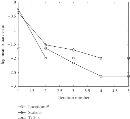
Cauchy distribution). Results are shown for varying sample lengths: 10, 100, and 1000. The experiments were run 1000 times for each block length, with the presented results the average on the trials. Mean final θ,σ, and p estimates are reported as well as the resulting MSE. To illustrate that the algorithm converges in a few iterations, given the proposed initialization, consider an an experiment utilizing data drawn from a GCDθ=0,σ=1, andp=1.5 distribution.Figure 3
reportsθ,σ,pestimate MSE curves. As in the previous case, 100 trials are averaged. Only the first five iteration points are shown, as the algorithms are convergent at that point.
To conclude this section, we consider the computational complexity of the proposed multiparameter estimation algo-rithm. The algorithm in total has a higher computational complexity than the FLOM, median, meridian, and myriad operators, sinceAlgorithm 1requires initial estimates of the location and the scale parameters. However, it should be noted that the proposed method estimatesallthe parameters
−3
1 1.5 2 3 3.5
Iteration number Location:θ
Scale:σ Tail:p
4 4.5 5
−2.5
−2
log
m
ean
squar
e
er
ror
−1.5
−1
−0.5
2.5 0
Figure3: Multiparameter estimation MSE iteration evolution for a GCD process with (θ,σ,P)=(0, 1, 1.5).
of the model, thus providing advantage over the aforemen-tioned methods that requirea prioriparameter tuning. It is straightforward to show that the computational complexity of the proposed method is O(N2), assuming the practical case in which the number of fixed-point iterations is N. The dominatingN2 term is the cost of selecting the input sample that minimizes the objective function, that is, the cost of evaluating the objective functionNtimes. However, if faster methods that avoid evaluation of the objective function for all samples (e.g., subsampling methods) are employed, the computational cost is lowered.
4. Robust Distance Metrics
This section presents a family of robust GCD-based error metrics. Specifically, the cost function of the M-GC estimator defined inSection 3.1is extended to define a quasinorm over Rmand a semimetric for the same space—the development is analogous toLpnorms emanating from the GGD family. We denote these semimetrics as the log-Lp (LLp) norms. (Note that for theσ = 1 and p = 1 case, this metric defines the log-Lspace in Banach space theory.)
Definition 5. Letu∈Rm, then theLL
pnorm ofuis defined as
uLLp,σ =
m
i=1 log
1 +|ui| p
σp
, σ >0. (34)
TheLLpnorm is not a norm in the strictest sense since it does not meet the positive homogeneity and subadditivity properties. However, it follows the positive definiteness and a scale invariant properties.
Proposition 2. Let c ∈ R,u,v ∈ Rm, and p,σ > 0. The
(i)uLLp,σ≥0, withuLLp,σ=0if and only ifu=0; (ii)cuLLp,σ= uLLp,δ, whereδ=σ/|c|;
(iii)u+vLLp,σ = v+uLLp,σ; (iv)letCp=2p−1. Then
u+vLLp,σ
≤
⎧ ⎨ ⎩
uLLp,σ+vLLp,σ, for0< p≤1, uLLp,σ+vLLp,σ+mlogCp, forp >1.
(35)
Proof. Statement 1 follows from the fact that log(1 +a)≥0 for alla≥0, with equality if and only ifa=0. Statement 2 follows from
m
i=1 log
1 +|cui| p
σp
=
m
i=1 log
1 + |ui| p
(σ/|c|)p
. (36)
Statement 3 follows directly from the definition of theLLp norm. Statement 4 follows from the well-known relation|a+ b|p ≤Cp(|a|p+|b|p),a,b∈R, whereC
pis a constant that depends only on p. Indeed, for 0 < p≤1 we haveCp =1, whereas forp >1 we haveCp=2p−1(for further details see [29] for example). Using this result and properties of thelog function we have
u+vLLp,σ=
m
i=1 log
1 +|ui+vi| p
σp
≤
m
i=1 log
1 +Cp
|ui|p+|vi|p
σp
=
m
i=1
logCp+ log
1 Cp
+
|ui|p+|vi|p
σp
≤
m
i=1
logCp+ log
1 +
|ui|p+|vi|p
σp
≤
m
i=1 log
1 +|ui| p
σp +
|vi|p
σp +
|ui|p|vi|p
σ2p
+mlogCp
=
m
i=1
log 1 +|ui| p
σp
!
1 +|vi| p
σp
!
+mlogCp
= uLLp,σ+vLLp,σ+mlogCp.
(37)
TheLLpnorm defines a robust metric that does not heav-ily penalize large deviations, with the robustness depending on the scale parameterσand the exponentp. The following lemma constructs a relationship between theLpnorms and theLLpnorms.
Lemma 2. For everyu ∈ Rm,0 < p ≤ 2, and σ > 0, the
following relations hold:
σpuLLp,σ≤ u p p≤σpm
euLLp,σ−1. (38)
Proof. The first inequality comes from the relation log(1 + x) ≤ x, for allx ≥ 0. Settingxi = |ui|p/σp and summing overiyield the result. The second inequality follows from
uLLp,σ=
m
i=1 log
1 +|ui| p
σp
≥max
i log
1 +|ui| p
σp
=log
1 +u p
∞
σp
. (39)
Noting thatu∞ ≤σ(euLLp,σ −1)1/ pandupp ≤mu∞p
for allp >0 gives the desired result.
The particular case p = 2 yields the well-known Lorentzian norm. The Lorentzian norm has desirable robust error metric properties.
(i) It is an everywhere continuous function.
(ii) It is convex near the origin (0 ≤ u ≤ σ), behaving similar to anL2cost function for small variations. (iii) Large deviations are not heavily penalized as in the
L1orL2norm cases, leading to a more robust error metric when the deviations contain gross errors.
Contour plots of select norms are shown in Figure 4
for the two-dimension case. Figures4(a)and4(c)show the L2 andL1 norms, respectively, while the LL2 (Lorentzian) and LL1 norms (for σ = 1) are shown in Figures 4(b)
and4(d), respectively. It can be seen fromFigure 4(b) that the Lorentzian norm tends to behave like theL2 norm for points within the unitaryL2ball. Conversely, it gives the same penalization to large sparse deviations as to smaller clustered deviations. In a similar fashion,Figure 4(d)shows that the LL1norm behaves like theL1norm for points in the unitary L1ball.
5. Illustrative Application Areas
This section presents four practical problems developed under the proposed framework: (1) robust filtering for power line communications, (2) robust estimation in sensor networks with noisy channels, (3) robust reconstruction methods for compressed sensing, and (4) robust fuzzy clustering. Each problem serves to illustrate the capabilities and performance of the proposed methods.
−10
−10 −5 0 5 10
−8
−6
−4
−2 0 2 4 6 8 10
(a)
−10
−10 −5 0 5 10
−8
−6
−4
−2 0 2 4 6 8 10
(b)
−10
−10 −5 0 5 10
−8
−6
−4
−2 0 2 4 6 8 10
(c)
−10
−10 −5 0 5 10
−8
−6
−4
−2 0 2 4 6 8 10
(d)
Figure4: Contour plots of different metrics for two dimensions: (a)L2, (b)LL2(Lorentzian), (c)L1, and (d)LL1norms.
fax services, and home networking is emerging in new com-munications industry technology. However, there remain considerable challenges for PLCs, such as communications channels that are hampered by the presence of large amplitude noise superimposed on top of traditional white Gaussian noise. The overall interference is appropriately modeled as an algebraic tailed process, with α-stable often chosen as the parent distribution [31].
While the M-GC filter is optimal for GCD noise, it is also robust in general impulsive environments. To compare the robustness of the M-GC filter with other robust filtering schemes, experiments for symmetric α-stable noise cor-rupted PLCs are presented. Specifically, signal enhancement for the power line communication problem with a 4-ASK
0.2 0.4 0.6 1 1.2 1.4 Tail parameter,α Median
FLOM
Meridian M-GC Myriad
1.6 1.8 10−15
10−10
No
rm
al
is
ed
M
S
E
10−5
0.8
Figure 5: Power line communication enhancement. MSE for different filtering structures as function of the tail parameterα.
The normalized MSE values for the outputs of the different filtering structures are plotted, as a function ofα, inFigure 5. The results show that the various methods per-form somewhat similarly in the less demanding light-tailed noise environments, but that the more robust methods, in particular the M-CG approach, significantly outperform in the heavy-tailed, impulsive environments. The time-domain results are presented inFigure 6, which clearly show that the M-GC is more robust than the other operators, yielding a cleaner signal with fewer outliers and well-preserved signal (symbol) transitions. The M-GC filter benefits from the optimization of the scale and tail parameters and therefore perform at least as good as the myriad and meridian filters. Similarly, the M-GC filter performs better than the FLOM filter, which is widely used for processing stable processes [9].
5.2. Robust Blind Decentralized Estimation. Consider next a set ofKdistributed sensors, each making observations of a deterministic source signalθ. The observations are quantized with one bit (binary observations), and then these binary observations are transmitted through a noisy channel to a fusion center whereθis estimated (see [32,33] and references therein). The observations are modeled asx=θ+n, wheren are sensor noise samples assumed to be zero-mean, spatially uncorrelated, independent, and identically distributed. Thus the quantized binary observations are
bk=1{xk∈(τ, +∞)} (40) fork = 1, 2,. . .,K, where τ is a real-valued constant and
1{·}is the indicator function. The observations received at the fusion center are modeled by
y=(2b−1) +w=m+w, (41) whereware zero-mean independent channel noise samples and the transformation mk = 2bk−1 is made to adopt a binary phase shift keying (BPSK) scheme.
The channel noise density function is denoted bywk ∼ fw(u). When this noise is impulsive (e.g., atmospheric noise or underwater acoustic noise), traditional Gaussian-based methods (e.g., least squares) do not perform well. We extend the blind decentralized estimation method proposed in [33], modeling the channel corruption as GCD noise and deriving a robust estimation method for impulsive channel noise scenarios. The sensor noise, n, is modeled as zero-mean additive white Gaussian noise with variance σ2
n, while the channel noise,w, is modeled as zero-location additive white GCD noise with scale parameter σw and tail constant p. A realistic approach to the estimation problem in sensor networks assumes that the noise pdf is known but that the values of some parameters are unknown [33]. In the following, we consider the estimation problem when the sensor noise parameterσnis known and the channel noise tail constantpand scale parameterσware unknown.
Instrumental to the scheme presented is the fact thatbk is a Bernoulli random variable with parameter
ψ(θ)Pr{bk=+1} =1−Fn(τ−θ), (42) where Fn(·) is the cumulative distribution function of nk. The pdf of the noisy observations received at the fusion center is given by
fy
y=ψ(θ)fw
y−1+*1−ψ(θ)+fw
y+ 1. (43) Note that the resulting pdf is a GCD mixture with mixing parametersψand [1−ψ]. To simplify the problem, we first estimateψ=ψ(θ) and then utilize the invariance of the ML estimate to determineθusing (42).
Using the log-likelihood function, the ML estimate of ψ∈(0, 1) reduces to
ψ=arg max ψ
K
k=1
logψ fw
yk−1
+*1−ψ+fw
yk+ 1
. (44)
The unknown parameter set for the estimation problem is {ψ,σw,p}. We address this problem utilizing the well known EM algorithm [28] and a variation ofAlgorithm 1in
Section 3.4. The followings are theE- and M-steps for the considered sensor network application.
E-Step. Let the parameters estimated at the j-th iteration be marked by a superscript (j) andΓ(j) = (σ(j)
w ,p(j)). The posterior probabilities are computed as
qk=
ψ(j)f w
yk−1|Γ(j)
ψ(j)f w
yk−1|Γ(j)
+*1−ψ(j)+f w
yk+ 1|Γ(j)
. (45)
M-Step. The ML estimates{ψ(j+1),Γ(j+1)}are given by
ψ(j+1)= 1 K
K
k=1
qk, Γ(j+1)=arg max
0 100 200 0
−1
−3
−2 1 2 3
300 400 500 600 700 800 900 1000 (a)
0 100 200 0
−1
−3
−2 1 2 3
300 400 500 600 700 800 900 1000 (b)
0 100 200 0
−1
−3
−2 1 2 3
300 400 500 600 700 800 900 1000 (c)
0 100 200 0
−1
−3
−2 1 2 3
300 400 500 600 700 800 900 1000 (d)
0 100 200 0
−1
−3
−2 1 2 3
300 400 500 600 700 800 900 1000 (e)
0 100 200 0
−1
−3
−2 1 2 3
300 400 500 600 700 800 900 1000 (f)
0 100 200 0
−1
−3
−2 1 2 3
300 400 500 600 700 800 900 1000 (g)
0 100 200 0
−1
−3
−2 1 2 3
300 400 500 600 700 800 900 1000 (h)
Figure6: Power line communication enhancement. (a) Transmitted signal, (b) Received signal corrupted byα-stable noiseα=0.4. Filtering results with: (c) Mean, (d) Median, (e) FLOMP=.25, (f) Myriad, (g) Meridian, (h) M-GC.
where
Λ(Γ)=
K
k=1 qkΥ
yk−1;Γ
+1−qk
Υyk+ 1;Γ
, (47)
whereΥ(u;Γ)=loga(p) + logσw−2p−1log(σwp+|u|p) and a(p) = pΓ(2/ p)/2(Γ(1/ p))2. We use a suboptimal estimate ofpin this case, choosing the value fromP= {0.5, 1, 1.5, 2}
that maximizes (46).
Numerical results comparing the derived GCD method, coined maximum likelihood with unknown generalized Cauchy channel parameters (MLUGC), with the Gaussian
channel-based method derived in [33], referred to as maxi-mum likelihood with unknown Gaussian channel parameter (MLUG), are presented in Figure 7. The MSE is used as a comparison metric. As a reference, the MSE of the binary estimator (BE) and the clairvoyant estimator (CE) (estimators in perfect transmission) are also included.
10−3
Contamination factor,p CE
BE
MLUG MLUGC
10−1
10−3
10−2
10−1
100
101
102
MSE
10−2
(a)
0.2 0.4 0.6 0.8 1 1.2 Tail parameter,α CE
BE
MLUG MLUGC 10−3
10−2
10−1
100
101
MSE
1.4 1.6 1.8
(b)
Figure7: Sensor network example with parameters:θ=1,τ=0,σn=1, andK=1000. Comparison of MLUGC, MLUG, BE, and CE. (a) Channel noise contaminatedp-Gaussian distributed withσ2
w=0.5. MSE as function of the of the contamination parameter,p. (b) Channel noiseα-stable distributed withσw=0.5. MSE as function of the tail parameter,α.
σ2
w =0.5 and varyingp(percentage of contamination) from 10−3 to 0.2. The results show a gain of at least an order of magnitude over the Gaussian-derived method. Results forα -stable distributed noise are shown inFigure 7(b), with scale parameterσw =0.5 and the tail parameter,α, varying from 0.2 to 2 (very impulsive to Gaussian noise). It can be observed that the GCD-derived method has a gain of at least an order of magnitude for allα. Furthermore, the MLUGC method has a nearly constant MSE for the entire range. It is of note that the MSE of the MLUGC method is comparable to that obtained by the MLUG (Gaussian-derived) for the especial case whenα = 2 (Gaussian case), meaning that the GCD-derived method is robust under heavy-tailed and light-tailed environments.
5.3. Robust Reconstruction Methods for Compressed Sensing.
As a third example, consider compressed sensing, which is a recently introduced novel framework that goes against the traditional data acquisition paradigm [34]. Take a set ofm sensors making observations of a signalx0 ∈ Rn. Suppose thatx0iss-sparse in some orthogonal basisΨ, and let{φi}mi=1 be a set of measurements vectors that are incoherent with the sparsity basis. Each sensor takes measurements projectingx0 onto{φi}mi=1and communicates its observation to the fusion center over a noisy channel. The measurement process can be modeled asy=Φx0+z, whereΦis anm×nmatrix with vectorsφias rows andzis white additive noise (with possibly impulsive behavior). The problem is how to estimatex0from the noisy measurementsy.
A range of different algorithms and methods have been developed that enable approximate reconstruction of sparse signals from noisy compressive measurements [35–39]. Most such algorithms provide bounds for the L2 reconstruction error based on the assumption that the corrupting noise is
bounded, Gaussian, or, at a minimum, has finite variance. Recent works have begun to address the reconstruction of sparse signals from measurements corrupted by outliers, for example, due to missing data in the measurement process or transmission problems [40,41]. These works are based on the sparsity of the measurement error pattern to first estimate the error and then estimate the true signal, in an iterative process. A drawback of this approach is that the reconstruction relies on the error sparsity to first estimate the error, but if the sparsity condition is not met, the performance of the algorithm degrades.
Using the arguments above, we propose to use a robust metric derived in Section 4 to penalize the residual and address the impulsive sampling noise problem. Utilizing the strong theoretical guarantees of basis pursuit (BP) L1 minimization, for sparse recovery of underdetermined systems of equations (see [34]), we propose the following nonlinear optimization problem to estimatex0fromy:
min
x∈Rnx1subject to,,y−Φx,,LL2,γ≤. (48) The following result presents an upper bound for the reconstruction error of the proposed estimator and is based on restricted isometry properties (RIPs) of the matrixΦ(see [34,42] and references therein for more details on RIPs).
Theorem 1(see [42]). Assume the matrix Φ meets an RIP, then for anys-sparse signalx0 and observation noise z with zLL2,γ≤, the solution to(48), denoted asx∗, obeys
,,x∗−x0,,
2≤Cs·2γ·
m(e−1), (49)
whereCsis a small constant.
Cauchy random variable with scale parameterσand location parameter zero. Assuming a Cauchy model for the noise vector yieldsEzLL2,γ =mElog{1 +γ−2Z2} =2mlog(1 + γ−1σ). We use this value forand setγas MAD(y).
Debiasing is achieved through robust regression on a subset of xindexes using the Lorentzian norm. The subset is set asI = {i:|xi|> α},α=λmaxi|xi|, where 0< λ <1. Thusx-I∈Rdis defined as
-xI=arg min x∈Rd
,,y−ΦIx,,
LL2,σ, (50)
whered = |I|. The final reconstruction after the regression (-x) is defined asx-Ifor indexes in the subsetIand zero outside I. The reconstruction algorithm composed of solving (48) followed by the debiasing step is referred to as Lorentzian basis pursuit (BP) [42].
Experiments evaluating the robustness of Lorentzian BP in different impulsive sampling noises are presented, comparing performance with traditional CS reconstruction algorithms orthogonal matching pursuit (OMP) [38] and basis pursuit denoising (BPD) [34]. The signals are synthetic s-sparse signals with s = 10 and length n = 1024. The number of measurements ism=128. For OMP and BPD, the noise bound is set as=mσ2, whereσis the scale parameter of the corrupting distributions. The results are averaged over 200 independent realizations.
For the first scenario, we consider contaminated p -Gaussian as the model for the sampling noise, with σ2 = 10−2, resulting in an SNR of 18.9 dB when no contamination is present (p = 0). The amplitude of the outliers is set as δ = 103, and p is varied from 10−3 to 0.5. The results are shown in Figure 8(a), which demonstrates that Lorentzian BP significantly outperforms BPD and OMP. Moreover, the Lorentzian BP results are stable over a range of contamination factors p, up to 5% of the measurements, making it a desirable method when measurements are lost or erased.
The second experiment explores the behavior of Lorentzian BP inα-stable environments. Theα-stable noise scale parameter is set as σ = 0.1 (γ in the traditional characterization) for all cases, and the tail parameter,α, is varied from 0.2 to 2, that is, very impulsive to the Gaussian case. The results are summarized inFigure 8(b), which shows that all methods perform poorly for small values ofα, with Lorentzian BP yielding the most acceptable results. Beyond α = 0.8, Lorentzian BP produces faithful reconstructions with an SNR greater than 20 dB, and often 30 dB greater than BPD and OMP results. Also of importance is that whenα=2 (Gaussian case), the performance of Lorentzian BP is comparable with that of BPD and OMP, which are Gaussian-derived methods. This result shows the robustness of Lorentzian BP under a broad range of noise models, from very impulsive heavy-tailed to light-tailed environments.
5.4. Robust Clustering. As a final example, we present a robust fuzzy clustering procedure based on theLLp metrics defined in Section 4, which is suitable for clustering data points involving heavy-tailed nonGaussian processes. Dave proposed the noise clustering (NC) algorithm to address
noisy data in [43, 44]. The NC approach is successful in improving the robustness of a variety of prototype-based clustering methods. This method considers the noise as a separate class and represents it by a prototype that has a constant distanceδ.
Let X = {xj}Nj=1,xj ∈ Rn, be a finite data set andC the given number of clusters. NC partitions the data set by minimizing the following function proposed in [43]:
J(Z)=
C
i=1 N
j=1
ui j
m
dxj,zi
+ N
j=1 δ
⎛ ⎝1−C
i=1 ui j
⎞ ⎠
m
, (51)
whereZ=[z1;. . .;zC] is a matrix whose rows are the cluster centers,m∈(1,∞) is a weighting exponent, andd(xj,zi) is the squaredL2distance from a data pointxjto the centerzi.
U=[ui j] is aC×Nmatrix, called a constraint fuzzy partition ofX, which satisfies [43]
ui j∈[0, 1] ∀i,j,
0< N
j=1
ui j< N ∀i,
C
i=1
ui j<1 ∀j.
(52)
Theui jweight represents the membership of thei-th sample to the j-th cluster. Minimization of the objective function with respect toU, subject to the constrains in (52), gives [43]
ui j= 1 C
k=1
⎡
⎣d
xj,zi
dxj,zk
⎤ ⎦
1/(m−1) +
⎡
⎣d
xj,zi
δ
⎤ ⎦
1/(m−1). (53)
Compared with the basic fuzzy C-means (FCM), the mem-bership constraint is relaxed toCi=1ui j<1. The second term in the denominator of (53) becomes large for outliers, thus yielding small membership values and improving robustness of prototype-based clustering algorithms.
To further improve robustness, we propose the applica-tion ofLLpmetrics in the NC approach. Substituting theLLp norm fordin (51) yields the objective function
J(Z)=
C
i=1 N
j=1
ui j
m,,
,xj−zi,,, LLp,σ+
N
j=1 δ
⎛
⎝1−
C
i=1 ui j
⎞ ⎠
m
. (54)
Given the objective function J(Z), a set of vectors {z}Ni=1 that minimize J(Z) must be determined. As in FCM, fix-point iterations are utilized to obtain the solution. We use a variation of the fixed point recursion proposed inSection 3.4
to achieve this goal. DifferentiatingJ(Z) with respect to each dimensionl of zs, treating theui j terms as constants, and setting it to zero yield the fixed point function. Thus the recursion algorithm can be written as
zsl(t+ 1)=
N
j=1wj(t)xjl
N
j=1wj(t)