Volume 2007, Article ID 25672,13pages doi:10.1155/2007/25672
Research Article
A Generalized Algorithm for Blind Channel Identification with
Linear Redundant Precoders
Borching Su and P. P. Vaidyanathan
Department of Electrical Engineering, California Institute of Technology, Pasadena, CA 91125, USA
Received 25 December 2005; Revised 19 April 2006; Accepted 11 June 2006
Recommended by See-May Phoong
It is well known that redundant filter bank precoders can be used for blind identification as well as equalization of FIR channels. Several algorithms have been proposed in the literature exploiting trailing zeros in the transmitter. In this paper we propose a generalized algorithm of which the previous algorithms are special cases. By carefully choosing system parameters, we can jointly optimize the system performance and computational complexity. Both time domain and frequency domain approaches of chan-nel identification algorithms are proposed. Simulation results show that the proposed algorithm outperforms the previous ones when the parameters are optimally chosen, especially in time-varying channel environments. A new concept of generalized signal richness for vector signals is introduced of which several properties are studied.
Copyright © 2007 B. Su and P. P. Vaidyanathan. This is an open access article distributed under the Creative Commons Attribution License, which permits unrestricted use, distribution, and reproduction in any medium, provided the original work is properly cited.
1. INTRODUCTION
Wireless communication systems often suffer from a prob-lem due to multipath fading which makes the channels frequency-selective. Channel coefficients are often unknown to the receiver so that channel identification needs to be done before equalization can be performed. Among techniques for identifying unknown channel coefficients, blind meth-ods have long been of great interest. In the literature many blind methods have been proposed based on the knowledge of second-order statistics (SOS) or higher-order statistics of the transmitted symbols [1,2]. These methods often need to accumulate a large number of received symbols until chan-nel coefficients can be estimated accurately. This requirement leads to a disadvantage when the system is working over a fast-varying channel.
A deterministic blind method using redundant filterbank precoders was proposed by Scaglione et al. [3] by exploiting trailing zeros introduced at the transmitter.Figure 1shows a typical linear redundant precoded system. Source sym-bols are divided into blocks with size M and linearly pre-coded intoP-symbol blocks which are then transmitted on the channel. It is well known that whenP ≥ M+L, where Lis the maximum order of the FIR channel, interblock in-terference (IBI) can be completely eliminated in absence of
noise. When the block sizeMincreases, the bandwidth effi -ciencyη=(M+L)/Mapproaches unity asymptotically. The deterministic method proposed in [3] (which we will call the SGB method) exploits trailing zeros with lengthLintroduced in each transmitted block and assumes the input sequence isrich. That is, the matrix composed of finite source blocks achieves full rank.
The method in [3] requires the receiver to accumulate at leastMblocks before channel coefficients can be identi-fied. This prevents the system from identifying channel co-efficients accurately when the channel is fast-varying, espe-cially when the block sizeM is large. More recently, Man-ton and Neumann pointed out that the channel could be identifiable with only two received blocks [4]. An algorithm based on viewing the channel identification problem as find-ing the greatest common divisor (GCD) of two polynomi-als is proposed in [5] (which we will call the MNP method). Eventhough it greatly reduces the number of received blocks needed for channel identification, the algorithm has much more computational complexity especially when the block sizeMis large.
s1(n)
s2(n)
sM(n)
Vector
s(n) Precoder
R(z) G(z)
u1(n)
u2(n)
uP(n)
Interleaving Blocking
Equalizer Channel
P
P
P
P
P
P u(n) y(n)
e(n)
H(z) z 1
z 1
z 1
z
z
z
Vector
y(n) y1(n)
y2(n)
yP(n)
s1(n)
s2(n)
sM(n)
Vector
s(n) .
. .
. .
. ... ...
. . .
. . .
Figure1: Communication system with redundant filter bank precoders.
complexity can be jointly optimized. The rest of the paper is organized as follows.Section 2describes the system struc-ture with linear precoder filter banks and reviews several existing blind algorithms. InSection 3we present the gen-eralized algorithm and derive the conditions on the input sequence under which the algorithm operates properly. In
Section 4we propose a frequency domain version of the gen-eralized algorithm. The concept ofgeneralized signal richness is introduced inSection 5 and some properties thereof are studied in detail. Simulation results and complexity analy-sis of both time and frequency domain approaches are pre-sented in Section 6. In particular, simulations under time-varying channel environments are presented to demonstrate the strength of the proposed algorithm against channel vari-ation. Finally, conclusions are made inSection 7. Some of the results in the paper have been presented at a conference [6].
1.1. Notations
Boldfaced lower-case letters represent column vectors. Bold-faced upper-case letters and calligraphic upper case letters are reserved for matrices. Superscripts as inAT andA† de-note the transpose and transpose-conjugate operations, re-spectively, of a matrix or a vector. All the vectors and ma-trices in this paper are complex-valued. In the figures “↑P” represents an expander and “↓P” a decimator [7].
If v = [v1 v2 · · · vMT] is an M ×1 column
vec-tor, thenT(v,q) denotes an (M+q−1)×qToeplitz ma-trix whose first row and first column are [v1 0 · · · 0] and [v1 v2 · · · vM 0 · · · 0T], respectively. For example,
T
⎛ ⎜ ⎜ ⎜ ⎝ ⎡ ⎢ ⎢ ⎢ ⎣
a1 a2 a3 a4
⎤ ⎥ ⎥ ⎥ ⎦, 3
⎞ ⎟ ⎟ ⎟ ⎠=
⎡ ⎢ ⎢ ⎢ ⎢ ⎢ ⎢ ⎢ ⎣
a1 0 0 a2 a1 0 a3 a2 a1 a4 a3 a2 0 a4 a3 0 0 a4
⎤ ⎥ ⎥ ⎥ ⎥ ⎥ ⎥ ⎥ ⎦
. (1)
2. PROBLEM FORMULATION AND
LITERATURE REVIEW
2.1. Redundant filter bank precoders
Consider the multirate communication system [8] depicted inFigure 1. The source symbolss1(n),s2(n),. . .,sM(n) may
come fromMdifferent users or from a serial-to-parallel op-eration on data of a single user. For convenience we consider the blocked versions(n) as indicated. The vectors(n) is pre-coded by aP×MmatrixR(z) whereP > M. The information with redundancy is then sent over the channelH(z). We as-sumeH(z) is an FIR channel with a maximum orderL, that is,
H(z)=
L
k=0
hkz−k. (2)
The signal is corrupted by channel noise e(n). The re-ceived symbols y(n) are divided into P × 1 block vec-tors y(n). The M ×P matrix G(z) is the channel equal-izer and s1(n),s2(n),. . .,sM(n) are the recovered symbol
streams. Also, for simplicity we definehas the column vector [h0 h1 · · · hLT]. We set
P=M+L, (3)
that is, the redundancy introduced in a block is equal to the maximum channel order.
2.2. Trailing zeros as transmitter guard interval
Suppose we choose the precoderR(z)=[R1
s1(n)
s2(n)
sM(n)
Vector
s(n)
R1
u1(n)
u2(n)
uM(n)
Vector
u(n)
Block of Lzeros
Noisee(n)
Channel P
P
P
P
P
P
P
P u(n) y(n)
H(z) z 1
z 1
z 1
z 1
z 1
z
z
z
Vector
y(n) y1(n)
y2(n)
yP(n)
. . .
. . . ...
. . .
. . .
Figure2: The zero-padding system with precoderR1.
Now, the received blocks can be written as
y(1) y(2) · · · y(J)
Ymatrix; sizeP×J
=HMR1
s(1) s(2) · · · s(J),
Smatrix; sizeM×J
(4)
whereHM = T(h,M) is the full-banded Toeplitz channel
matrix. As long as vectorhis nonzero, the matrixHM has
full column rankM. Now, we assume the signals(n) isrich, that is, there exists an integerJ such that the matrix S has full row rank M. Since R1 is an M×M invertible matrix, we conclude that theP×J matrixY has rankM. So there existLlinearly independent vectors that are left annihilators ofY. In other words, there exists aP×LmatrixU0such that U†0Y=UHMR1S=0. Now thatR1Shas rankM, this implies
U†0HM=0. (5)
The channel coefficientshcan then be determined by solving (5). In practice wherechannel noiseis present, the computa-tion of the annihilators is replaced with the computacomputa-tion of the eigenvectors corresponding to the smallestLsingular val-ues ofY. In this and the following sections, the channel noise term is not shown explicitly.
Note that this algorithm [3] works under the assumption thatShas full row rankM. ObviouslyJ ≥M is a necessary condition for this assumption. This means the receiver must accumulate at leastMblocks (i.e., a duration ofM(M+L) symbols) before channel identification can be performed. This could be a disadvantage when the system is working over a fast-varying channel.
2.3. The GCD approach
Another approach proposed in [5] requires only two received blocks for blind channel identification. Recall that the chan-nel is described byy=HMu=T(h,M)u, or
⎡ ⎢ ⎢ ⎢ ⎢ ⎣
y1 y2 .. . yP
⎤ ⎥ ⎥ ⎥ ⎥ ⎦=
⎡ ⎢ ⎢ ⎢ ⎢ ⎢ ⎢ ⎢ ⎢ ⎢ ⎢ ⎢ ⎣
h0 0
h1 . .. ..
. h0 hL h1 . .. ...
0 hL
⎤ ⎥ ⎥ ⎥ ⎥ ⎥ ⎥ ⎥ ⎥ ⎥ ⎥ ⎥ ⎦ ⎡ ⎢ ⎢ ⎢ ⎢ ⎣
u1 u2 .. . uM
⎤ ⎥ ⎥ ⎥ ⎥
⎦. (6)
By multiplying [1 x x2 · · · xP−1] to both sides of (6), we obtain
y(x)=h(x)u(x), (7)
where
y(x)
P−1
k=0
yk+1xk, h(x)
L
k=0 hkxk,
u(x)
M−1
k=0 uk+1xk
(8)
To compute the GCD of y1(x) and y2(x), we first con-struct a (2P−1)×2Pmatrix [9]
YP ⎡ ⎢ ⎢ ⎢ ⎢ ⎢ ⎢ ⎢ ⎢ ⎢ ⎢ ⎢ ⎢ ⎢ ⎢ ⎢ ⎣
y11 0 · · · 0 y21 0 · · · 0 y12 y11 . .. ... y22 y21 . .. ...
..
. y12 . .. 0 ... y22 . .. 0
y1P ... y11 y2P ... y21 0 y1P y12 0 y2P y22
..
. . .. ... ... ... . .. ... ... 0 · · · 0 y1P 0 · · · 0 y2P
⎤ ⎥ ⎥ ⎥ ⎥ ⎥ ⎥ ⎥ ⎥ ⎥ ⎥ ⎥ ⎥ ⎥ ⎥ ⎥ ⎦ . (9)
One can verify that
YP= ⎡ ⎢ ⎢ ⎢ ⎢ ⎢ ⎢ ⎢ ⎢ ⎢ ⎢ ⎢ ⎣
h0 0
h1 . .. ..
. h0 hL h1 . .. ...
0 hL
⎤ ⎥ ⎥ ⎥ ⎥ ⎥ ⎥ ⎥ ⎥ ⎥ ⎥ ⎥ ⎦
matrixHM+P−1 size(2P−1)×(M+P−1)
⎡ ⎢ ⎢ ⎢ ⎢ ⎢ ⎢ ⎢ ⎢ ⎢ ⎢ ⎢ ⎣
u11 0 u21 0
u12 . .. u22 . .. ..
. u11 ... u21 u1M u12 u2M u22 . .. ... . .. ...
0 u1M 0 u2M
⎤ ⎥ ⎥ ⎥ ⎥ ⎥ ⎥ ⎥ ⎥ ⎥ ⎥ ⎥ ⎦ matrixU size(M+P−1)×2P
.
(10)
Whenu1(x) andu2(x) are coprime to each other, it can be shown that the matrix Uhas full rank M+P−1 (see
Section 5). SinceHM+P−1 =T(h,M+P−1) also has rank M+P−1, rank(YP)=M+P−1 and henceYP hasLleft
annihilators (i.e., there exists a (2P−1)×LmatrixU0such thatU†0Y = 0). These annihilators are also annihilators of each column of matrixHM+P−1, and we can therefore, in ab-sence of noise, identify channel coefficientsh0,h1,. . .,hLup
to a scalar ambiguity. In presence of noise, the columns of U0would be selected as the eigenvectors associated with the smallest singular values ofYP.
2.4. Connection to the earlier literature
The MNP method described above can be viewed as a dual version of the subspace methods proposed in the earlier lit-erature in multichannel blind identification [10,11]. In the subspace method in [11], the single source can be estimated as the GCD of the received data from two (more generallyN) different antennas. The MNP method [5] swaps the roles of data blocks and multichannel coefficients.
3. A GENERALIZED ALGORITHM
In this section we propose a generalized algorithm of which each of the two algorithms described in the previous section is a special case. Comparing the two algorithms described above, we find that the MNP approach needs much fewer received blocks for blind identifiability. However, it has more computational complexity. Each received block is repeatedP times to build a big matrix. Using the generalized algorithm, we can choose the number of repetitions and the number of
received blocks freely as long as they satisfy a certain con-straint.
3.1. Algorithm description
Observe (6) again and note that it can be rewritten as T(y,Q)=T(h,M+Q−1)T(u,Q), (11) whereT(·,·) is defined as in (1). HereQcan be any positive integer. Note that in the MNP methodQis chosen asP, as described in the previous section. Suppose the receiver gath-ersJblocks withJ ≥ 2. Then we haveY(QJ) =HM+Q−1U(QJ),
where
Y(QJ)=Ty(1),Q Ty(2),Q · · · Ty(J),Q, HM+Q−1=T(h,M+Q−1),
(12)
U(QJ)=Tu(1),P · · · Tu(J),P. (13)
Note thatU(QJ) has size (M+Q−1)×QJandY(QJ)has size (P+Q−1)×QJ. For notational simplicity, from now on we will use subscriptQas inNQto denoteNQ=N+Q−1 where
Ndenotes a positive integer. In particular, MQ=M+Q−1,
PQ=P+Q−1.
(14)
Notice that they still have the relationshipPQ=MQ+L.
Assume now the matrixU(QJ)has full row rankMQ. Taking
singular-value decomposition (SVD) ofY(QJ)we have
Y(QJ)=Ur U0 Σ 0 Vr V0 †
. (15)
The size ofΣisMQ×MQsince bothHMQ andU (J)
Q have full
rankMQ. The columns of theMQ×LmatrixU0are left
an-nihilators of matrixY(J)and also ofHsinceU(J)has full row rank. Suppose
U†0=
⎡ ⎢ ⎢ ⎢ ⎢ ⎣
u11 u12 · · ·u1,P+Q−1 u21 u22 · · ·u2,P+Q−1
..
. ...
uL1 uL2 · · ·uL,P+Q−1
⎤ ⎥ ⎥ ⎥ ⎥
⎦. (16)
Form the Hankel matrices
Uk ⎡ ⎢ ⎢ ⎢ ⎢ ⎣
uk1 uk2 · · · uk,L+1 uk2 uk3 · · · uk,L+2
..
. ...
uk,MQ uk,MQ+1 · · · uk,PQ
⎤ ⎥ ⎥ ⎥ ⎥ ⎦ (17)
fork, 1≤k≤L. Then we have
⎡ ⎢ ⎢ ⎢ ⎢ ⎣ U1 U2 .. . UL ⎤ ⎥ ⎥ ⎥ ⎥ ⎦
Umatrix; sizeLMQ×(L+1)
h=0. (18)
Vector
v(n)
Vector
vQ(n)
N N
N
N
NQ NQ
NQ
NQ
z 1
z 1
Q
Q 1
⎡ ⎣IN
0
⎤ ⎦
1
Q 2
⎡ ⎢ ⎢ ⎣
0
IN 0
⎤ ⎥ ⎥ ⎦
Q 1
⎡ ⎣0
IN
⎤ ⎦
. .
. .
. .
. . .
Figure3:Q-repetition and shifting operation.
3.2. Q-repetition and shifting operation
As we can see in the previous section, the repetition and shifting operation on a vector signal is crucial in the gener-alized algorithm.Figure 3gives a block diagram of this oper-ation. For future notational convenience, the subscriptQas invQ(n) denotes the result of this operation on a vector
sig-nal. By viewing (11) and applying this operation ony(n) and u(n), we obtain the relationship
yQ(n)=HM+Q−1uQ(n)
for any positive integerQ.
3.3. Special cases of the algorithm
The blind channel identification algorithm described above uses two parameters: (a) the number of received blocksJ; (b) the number of repetitions per blockQ. A number of points should be noted here:
(1) the algorithm works for anyJandQas long asU(QJ)has full row rankMQ.This is the only constraint for choosing
parametersJandQ;
(2) note that if we choose Q = 1 andJ ≥ M, then the algorithm reduces to theSGB algorithm[3];
(3) if we chooseQ = PandJ = 2, it becomes theMNP algorithm[5].
So both the SGB method and the MNP method are a special case of the proposed algorithm. SinceU(QJ) has size MQ ×QJ,U(QJ) having full row rank implies QJ ≥ MQ =
M+Q−1, or
Q≥M−1
J−1 . (19)
Also note that we cannot chooseJ =1 sinceU(QJ)can never have full rank unless the block sizeM=1. This is consistent with the theory that two blocks are required for blind chan-nel identification [4]. While the inequality (19) is a necessary
condition forU(QJ)to have full rank, it is not sufficient because it also depends on the values of entries ofu(n). Nevertheless, when inequality (19) is satisfied, the probability ofU(QJ) hav-ing full rank is usually close to unity in practice, especially when a large symbol constellation is used. Thus,
Q=
M−1 J−1
(20)
appears to be a selection that minimizes the computational cost given the number of received blocksJ. A detailed study on the conditions forU(QJ)to have full rank is presented in
Section 5.
WhenJ =2,Qcan be chosen as small asM−1 rather thanP. If we takeJ=3,Q= (M−1/2)makes the matrix Ytwice smaller. We can choose Q = 1 only whenJ ≥ M. This coincides with the SGB algorithm which uses a richness assumption [3].
4. FREQUENCY DOMAIN APPROACH
In this section we slightly modify the blind identification al-gorithm and directly estimate the frequency responses of the channel at different frequency bins and equalize the channel in the frequency domain. We call the modified algorithm fre-quency domain approach. Some of the ideas come from [12]. The receiver structure for the frequency domain approach is shown inFigure 4. To demonstrate how this system works, observe thePQ×MQfull-banded Toeplitzchannel matrix
HMQ=T
h,MQ
. (21)
Define a row vectorvT
ρ = [1 ρ−1 · · · ρ−(PQ−1)] withρ a
nonzero complex number. Due to full-banded Toeplitz struc-ture ofHMQ, we have
vT ρHMQ =
H(ρ) ρ−1H(ρ) · · · ρ−(MQ−1)H(ρ), (22)
whereH(ρ)=L
k=0hkρ−kis the channelz-transform
evalu-ated atz=ρ.
LetNbe chosen as an integer greater than or equal toPQ,
and letρ1,ρ2,. . .,ρN be distinct nonzero complex numbers.
Consider anN×PQmatrixVN×PQwhoseith row isvTρi:
VN×PQ =
⎡ ⎢ ⎢ ⎢ ⎢ ⎢ ⎢ ⎢ ⎣
1 ρ−11 ρ1−2 · · · ρ −(PQ−1) 1
1 ρ−1
2 ρ2−2 · · · ρ −(PQ−1) 2 ..
.
1 ρ−1
N ρN−2 · · · ρ
−(PQ−1)
N ⎤ ⎥ ⎥ ⎥ ⎥ ⎥ ⎥ ⎥ ⎦
. (23)
It is easy to verify that
VN×PQHMQ =ΛN
⎡ ⎢ ⎢ ⎢ ⎢ ⎢ ⎢ ⎢ ⎣
1 ρ−11 · · · ρ −(MQ−1) 1
1 ρ−1
2 · · · ρ− (MQ−1) 2 .. .
1 ρ−1
N · · · ρ
−(MQ−1)
N ⎤ ⎥ ⎥ ⎥ ⎥ ⎥ ⎥ ⎥ ⎦
,
VN×MQmatrix
Q-repetition and
shifting VN
PQ
P
P
P y(n) z
z
z
Vector
y(n) y1(n)
y2(n)
yP(n)
Vector
yQ(n)
yQ1(n)
yQ2(n)
yQPQ(n)
Vector
z(n) z1(n)
z2(n)
zN(n)
. .
. ... .
. .
Figure4: Receiver structure for frequency domain approach.
where
ΛN=diag
Hρ1
Hρ2
· · · HρN
diaghN
(25)
is a diagonal matrix with frequency domain channel coeffi -cients as the diagonal entries. Now, when we gather receiving blocks and repeat them as in (12), we get the following ma-trix:
Y(QJ)=T(y(1),Q) T(y(2),Q) · · · Ty(J),Q. (26)
Since we haveY(QJ) = HMQU (J)
Q in absence of noise, by
multiplyingVN×PQ andY (J)
Q , we have
Z=VN×PQY (J)
Q =VN×PQHMQU (J)
Q =ΛNVN×MQU (J)
Q . (27)
Recall that rank(Y(QJ))=rank(U(QJ))=MQ. Sinceρ1,ρ2,. . .,ρN
are all distinct, the matrixZhas the same rank asY(QJ). The dimension of the null space of matrixZis henceN−MQ. By
performing SVD onZ, we can find theseN−MQ left
anni-hilators ofZ, which are also annihilators ofΛNVN×MQ. There exists an (N−MQ)×NmatrixU†0 such thatU†0Z=0. Since U(QJ)has full rank, this implies
U†0ΛNVN×MQ =0. (28)
Suppose
U†0=
⎡ ⎢ ⎢ ⎢ ⎢ ⎣
u11 u12 · · · u1N
u21 u22 · · · u2N
..
. ... ...
uN−MQ,1 uN−MQ,2 · · · uN−MQ,N
⎤ ⎥ ⎥ ⎥ ⎥
⎦. (29)
Then by observing thei jth entry of (28), we have
u†i jh†N =0 (30)
for alli,j, 1≤ i≤N−MQ and 1≤ j ≤MQ, whereui j =
[ui1ρ1−(j−1) ui2ρ2−(j−1) · · · uiNρN−(j−1)]†. HerehNis the row
vector in (25). Form theMQ×Nmatrices
Ui= ⎡ ⎢ ⎢ ⎢ ⎢ ⎢ ⎢ ⎢ ⎣
ui1 ui2 · · · uiN
ui1ρ−11 ui2ρ−21 · · · uiNρ−N1
ui1ρ−12 ui2ρ−22 · · · uiNρ−N2
.. .
ui1ρ1−(MQ−1) ui2ρ2−(MQ−1) · · · uiNρN−(MQ−1) ⎤ ⎥ ⎥ ⎥ ⎥ ⎥ ⎥ ⎥ ⎦
,
(31)
and letU =[UT
1 UT2 · · · UTN−MQ]T. Then from (30) we haveUhN = 0. Then the frequency domain channel coeffi
-cientshN can be estimated by solving this equation. After the
frequency domain channel coefficients are estimated, the re-ceived symbols can be equalized directly in the frequency do-main, as in DMT systems.
Recall that we have the freedom to chooseNas any inte-ger greater than or equal toPQand the values ofρi, 1≤i≤N
as any nonzero complex number in thez-domain. In this pa-per, we useN=PQand
ρk=exp j
2kπ N
!
, k=0, 1,. . .,N−1. (32)
Note that sinceH(z) is an Lth order system, there are at mostLvalues amongH(ρi) which can be zero (channel
nulls). By choosingN ≥ PQ, there are at leastMQ nonzero
values among H(ρi), i = 1, 2,. . .,PQ. In practice we can
choose to equalize the received symbols in frequency bins as-sociated with the largest MQ frequency responses H(ρi) to
enhance the system performance. This provides resistance to channel nulls.
5. GENERALIZED SIGNAL RICHNESS
For the generalized blind channel identification method pro-posed in this paper to work properly, the matrix U(QJ) de-fined in (13) must have full row rank for given parame-tersJandQ. An obvious necessary condition has been pre-sented as inequality (19) inSection 3. The sufficiency, how-ever, depends on the content of signal u(n). When Q = 1 and u(n) is rich, then there exists J such that U(QJ) = [u(0) u(1) · · · u(J−1)] has full rank. WhenQ >1,u(n) requires another kind of richness property so thatU(QJ) has full rank for a finite integerJ. We call this property the gener-alized signal richnessand define it as follows.
Definition 1. AnM×1 sequenceu(n),n ≥ 0 is said to be (1/Q)-richif there exists a finite integerJsuch that the (M+ Q−1)×JQmatrix
U(QJ)=Ts(0),Q Ts(1),Q · · · Ts(J),Q (33)
has full row rankM+Q−1.
5.1. Measure of generalized signal richness
Lemma 1. If anM×1sequences(n)is(1/Q)-rich, thens(n) is(1/(Q+ 1))-rich.
Proof. See the appendix.
Lemma 1 states a basic property of generalized signal richness: the smaller the value ofQis, the “stronger” the con-dition of (1/Q)-richness is. For example, if anM×1 sequence s(n) is 1-rich, or simplyrich, then it is (1/Q)-rich for any pos-itive integerQ. On the contrary, a (1/2)-rich signals(n) is not necessarily 1-rich. We can thus define a measure of general-ized signal richness for a givenM×1 sequences(n) as follows.
Definition 2. Given anM×1 sequences(n),n≥0, thedegree of nonrichnessofs(n) is defined as
Qminmin
Q s(n) is
1 Q-rich
!
. (34)
Recall that the larger the degree of nonrichnessQminis, the weaker the richness of the signal s(n) is. If s(n) is not (1/Q)-rich for anyQ, thenQmin= ∞. The property of an in-finite degree of nonrichness can be described in the follow-ing lemma. We use the notationpM(x) to denote the column
vector:
pM(x)=
1 x x2 · · · xM−1T
. (35)
Lemma 2. Consider anM×1 sequences(n). The following statements are equivalent:
(1) s(n)is not(1/Q)-rich for anyQ;
(2) the degree of nonrichness ofs(n)is infinity; (3) either there exists a complex numberαsuch that
[1 α · · · αM−1]is an annihilator ofs( n)or [0 · · · 0 1]is an annihilator ofs(n);
(4) either polynomialspn(x)=pMT(x)s(n), n≥0share
a common zero (atα) or their orders are all less than M−1.
Proof. See the appendix.
Note that the statement [0 · · · 0 1] is an annihilator ofs(n) in condition (3) and the statement that polynomials pn(x) have orders less thanM−1 in condition (4) can be
interpreted as the special situation when the common zeroα is at infinity.
If anM×1 sequence s(n) has a finite degree of non-richness, ors(n) is (1/Q)-rich for some integerQ, then it can be shown that the maximum possible value ofQminisM−1, as described in the following lemma.
Lemma 3. IfM >1and anM×1sequences(n)is not(1/(M− 1))-rich, then it is not(1/Q)-rich for anyQ.
Proof. See the appendix.
WithLemma 3, we can see that for anM×1 sequence s(n), the possible values of the degree of non-richnessQmin
are 1, 2,. . .,M −1, and ∞. (1/(M −1))-richness is thus the weakest form of generalized richness. When using the MNP method [9], this weakest form of generalized richness is very crucial. If this weakest form of richness of s(n) is not achieved, then by Lemma 2s(n) has an infinite degree of non-richness and polynomialspTM(x)s(n) have a common factor (x−α). Then as inSection 2.3, when we take GCD of the polynomials representing the received blocks, the receiver would be unable to determine whether the factor (x−α) be-longs to the channel polynomial or is a common factor of the symbol polynomials.Therefore, if the input signals(n)has in-finite degree of non-richness, all methods proposed in this paper will fail for allQ.
Furthermore, the MNP method proposed in [5] usesQ= P. UsingLemma 3, we see that usingQ=M−1 is sufficient if we are computing the GCD of polynomials representing received blocks and the following two conditions are true: (1) the GCD is known to have a degree less than or equal toL; (2) the degree of each symbol polynomial is less than or equal to M−1. UsingQ=Pnot only is computationally unnecessary, but also, as we will see in simulation results inSection 6, has sometimes a worse performance than usingQ = M−1 in presence of noise.
The sufficiency ofQ=M−1 can also be understood from the point of view of polynomial theory. Suppose polynomials a(x) andb(x) have degrees less than or equal to P−1 and have a greatest common denominatord(x) whose degree is less than or equal toL. Supposea(x)=d(x)a1(x) andb(x)= d(x)b1(x) and botha1(x) andb1(x) have degrees less than or equal toM−1 and they are coprime to each other. Then there exists polynomialsp(x) andq(x) whose degree are less than or equal toM−2 such that 1= p(x)a1(x) +q(x)b1(x) and thusd(x)=p(x)a(x) +q(x)b(x).
5.2. Connection to earlier literature
An earlier proposition mathematically equivalent toLemma 3 has been presented in the single-input-multiple-output (SIMO) blind equalization literature [10,13]. We review it here briefly.
Proposition 1. Leth[n]beJ×1vectors. Suppose aQJ×(Q+ M−1)block Toeplitz matrix
TQ(h)
=
⎡ ⎢ ⎢ ⎢ ⎢ ⎢ ⎣
h[0] h[1] · · · h[M−1] 0 · · · 0 0 h[0] h[1] · · · h[M−1] . .. ...
..
. . .. ... . .. . .. . .. 0 0 · · · 0 h[0] h[1] · · · h[M−1]
⎤ ⎥ ⎥ ⎥ ⎥ ⎥ ⎦
(36)
ThenTQ(h)has full column rank if and only if
h(z)
M
i=0
h[i]z−i =0, ∀z. (37)
Hereh[n] was used to refer to the impulse response of aJ×1 channel.Qstands for the observation period in the multiple-channel receiver end. Conditions (1) and (2) imply that the channel has finite impulse response. Condition (3) can be met by increasing the observation periodQ. While this old proposition focuses on the coefficients of multiple chan-nels rather than values of transmitted symbols, it is mathe-matically equivalent to the statement thats(n) is (1/(M− 1))-rich if and only if polynomialspTM(x)s(n) do not share com-mon zeros. The case ofQ < M−1, however, has not been considered earlier in the literature, to the best of our knowl-edge.
5.3. Remarks on generalized signal richness
In this section we introduced the concept of generalized sig-nal richness. Given anM×1 signals(n), n≥ 0, thedegree of non-richnessQminwas defined. For an input signal with a degree of non-richnessQmin, we can choose any
Q≥Qmin (38)
and some finiteJfor the generalized algorithm proposed in
Section 3to work properly. The possible values ofQminare 1, 2,. . .,M−1, and∞. Ifs(n) has an infinite degree of non-richness, the algorithm proposed in this paper will fail for all Q. The degree of non-richness of a signals(n) directly depends on its content. A deeper study of degree of non-richness will be presented elsewhere [14].
6. SIMULATIONS AND DISCUSSIONS
In this section, several simulation results, comparisons, and discussions will be presented. We will first test our proposed method and compare it with the existing methods [3,5] de-scribed inSection 2. Secondly, we will compare the perfor-mances of time domain versus frequency domain approaches and show that under some channel conditions the frequency domain approach outperforms the time domain approach. Finally, we will analyze and compare the computational com-plexity of algorithms proposed in this paper.
6.1. Simulations of time domain approaches
A Rayleigh fading channel of orderL= 4 is used. The size of transmitted blocks isM=8 and received block size isP= M+L=12. The normalized least squared channel estimation error, denoted asEch, is used as the figure of merit for channel
identification and is defined as follows:
Ech=
h−h2
h2 , (39)
45 40 35 30 25 20 15 10
SNR (dB) 10 5
10 4
10 3
10 2
10 1
100
101
N
o
rm
aliz
ed
ch
annel
M
SE
M=8;L=4
J=2,Q=12 (GCD) J=2,Q=1 (SGB) J=2,Q=8
J=10,Q=12 (GCD) J=10,Q=1 (SGB) J=10,Q=2
Figure5: Normalized least squared channel error estimation.
45 40 35 30 25 20 15 10
SNR (dB) 10 7
10 6
10 5
10 4
10 3
10 2
10 1
100
BER
M=8;L=4
J=2,Q=12 (GCD) J=2,Q=1 (SGB) J=2,Q=8
J=10,Q=12 (GCD) J=10,Q=1 (SGB) J=10,Q=2
Figure6: Bit error rate.
45 40 35 30 25 20 15 10
SNR (dB) 10 5
10 4
10 3
10 2
10 1
100
N
o
rm
aliz
ed
ch
annel
M
SE
M=8;L=4
FD 9 blocksQ=1 TD 9 blocksQ=1 FD 9 blocksQ=2 TD 9 blocksQ=2
Figure7: Normalized least squared channel error estimation.
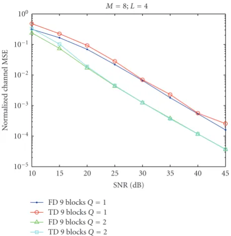
6.2. Simulations of frequency domain approaches
Figure 7 shows the comparison of frequency domain ap-proach and time domain apap-proach under the channel coeffi -cientsH(z)=1−jz−1+ (−1 + 0.01j)z−2+ (0.01 +j)z−3− 0.01jz−4.
For frequency domain approach, the normalized least squared channel error is defined as
Ech=
h−h2
h2 , (40)
where
h=Hρ1
Hρ2
· · · HρN
(41)
andh is the estimation ofh. Simulation results show that frequency domain approach outperforms time domain ap-proach especially when the noise level is high. While the fre-quency domain approach does not in general beat the time domain approach for a random channel, it has been consis-tently observed that frequency domain approach performs better than time domain approach when the last channel co-efficienth(L) has a small magnitude (i.e., at least one zero of H(z) is close to the origin).
Since we have the freedom to choose values of coefficients ρi, the receiver can adjust ρi dynamically according to the
a priori knowledge of the approximated channel zero loca-tions. This is especially useful when the channel coefficients are changing slowly from block to block.
6.3. Complexity analysis
For the algorithms presented inSection 3, the SVD computa-tion dominates the computacomputa-tional complexity. The number of blocksJ, the number of repetitions per blockQ, and the received block sizePdecide the size of the matrix on which SVD is taken. The complexity of SVD operation on ann×m matrix [15] is on the order ofO(mn2) withm≥n. SinceY(J)
Q
has size (P+Q−1)×QJ, the complexity isO(QJ(P+Q−1)2). We can see that the complexity can be greatly reduced by choosing a smallerQ. Recall that the SGB method [3] uses Q=1 and the MNP method [5] usesQ=P. We thus have the following arguments:
(i) the MNP method has a complexity around 4P times the complexity of the SGB method for anyJ. A choice ofQbetween 1 andPcould be seen as a compromise between system performance and complexity; (ii) when J is large, we have the freedom to choose a
smallerQ, as explained in the previous section.
For the frequency domain approach presented inSection 4, an additional matrix multiplication is required. This de-mands extra computational complexity of the order of O(JP2
Q). However, if the values ρi are chosen as equally
spaced on the unit circle, an FFT algorithm can be ex-ploited and the computational complexity will be reduced to O(JPQlogPQ) and is negligible compared to the complexity
of SVD operations.
6.4. Simulations for time-varying channels
In this section, we demonstrate the capability of the proposed generalized blind identification algorithm in time-varying channels environments. The received symbols can be ex-pressed as
y(n)=
L
k=0
h(n,k)x(n−k), (42)
where the (L+ 1)-tap channel coefficientsh(n,k) vary as the time indexnchanges. We generate the channel coefficients as follows. During a time intervalT, the channel coefficients change fromh1(k) toh2(k), whereh1(k) andh2(k), 0≤k≤ Lrepresent two sets of (L+ 1)-tap independent coefficients. The variation of the coefficient is done by linear interpolation such that
h(n,k)=
⎧ ⎪ ⎪ ⎪ ⎪ ⎪ ⎨ ⎪ ⎪ ⎪ ⎪ ⎪ ⎩
h1(k), ifn=0,
h2(k), ifn=T, T−n
T h1(k) + n
Th2(k) otherwise.
(43)
Table1: Coefficients for the time-varying channel.
k h1(k) h2(k)
0 −0.6563 + 0.7059i −1.2519 + 0.2295i
1 −0.6534 + 1.1774i 0.9347 + 0.1237i
2 −0.4229−0.2362i 0.0346−0.6180i
3 0.2145−0.2207i 0.7272−1.4084i
4 −0.1478 + 0.2802i 0.8612 + 0.3455i
channel error is defined as
Ech=
h−h2
h2 , (44)
wherehis the estimated channel andhis the averaged coef-ficients during the time the channel is being estimated:
h= 1 JP
n0+JP−1
n=n0
h(n, 0) h(n, 1) · · · h(n,L)T. (45)
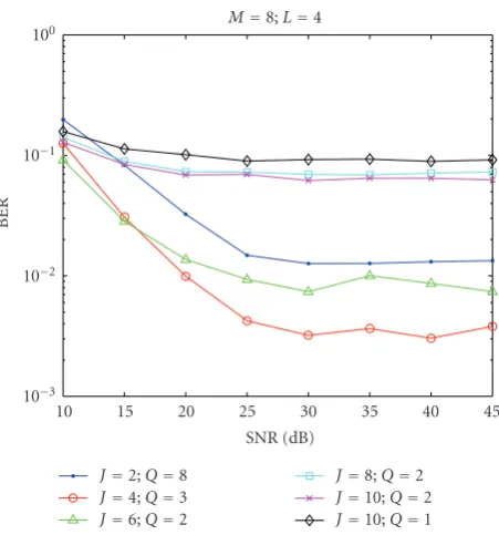
InFigure 8we see that whenJ = 10, the time range is too large for the algorithm to estimate the time-varying chan-nel accurately. The performance forJ =2 is much better in high SNR region because the channel does not vary too much during the time of two blocks. However, in low SNR region the performance forJ =2 becomes bad. The case forJ =4 has the best performance among all other choices because the channel does not vary too much during the duration of four receiving blocks, and more data are available for accurate es-timation. This simulation result provides clues about how we can choose the optimalJ: if the channel variation is fast (Tis smaller) we need a smallerJwhile we can use a largerJwhen Tis larger.
6.5. Remarks on choosing the optimal parameters
According to the simulations results above, we summarize here a general guideline to choose a set of optimal param-eters in practice.
(1) When the channel is constant and for a fixedQ, a larger J appears to have a better performance (as shown in
Figure 5) since more data are available for accurate es-timation.
(2) When the channel is time-varying, the optimal choice ofJ depends on the speed of channel variation. Sim-ulation results in Figures 8 and9 suggest when the channel coefficients completely change inNblocks, a choice ofJ≈N/4 could be appropriate.
(3) SupposeJis given, a choice ofQas the smallest inte-ger that satisfies inequality (19) often has a satisfactory performance. A slightly largerQcan sometimes be bet-ter (seeFigure 5forJ=10) at the expense of a slightly increased complexity. However, if Qis too large, the performance could be even worse (seeFigure 5forJ= 2,Q=12).
The guidelines above are given by observing the simulation results. An analytically optimal set ofJ andQis still under investigation.
45 40 35 30 25 20 15 10
SNR (dB) 10 2
10 1
100
101
N
o
rm
aliz
ed
ch
annel
M
SE
M=8;L=4
J=2;Q=8 J=4;Q=3 J=6;Q=2
J=8;Q=2 J=10;Q=2 J=10;Q=1
Figure 8: Normalized channel MSE performance for a time-varying channel.
45 40 35 30 25 20 15 10
SNR (dB) 10 3
10 2
10 1
100
BER
M=8;L=4
J=2;Q=8 J=4;Q=3 J=6;Q=2
J=8;Q=2 J=10;Q=2 J=10;Q=1
Figure9: Bit error rate performance for a time-varying channel.
6.6. Noise handling for largeJ
It should be noted that whenJis very large (andQ=1), the proposed method behaves like a traditional subspace method using second-order statistics. Suppose
whereE(J) is composed ofJ columns of noise vectorse(n). The autocorrelation matrix of received blocks can be esti-mated as
Ry y=E &
y(n)y†(n)'≈1 JY
(J)Y(J)†. (47)
If the input signal and channel noise are uncorrelated, we can writeRy yas
Ry y=HRuuH†+Ree, (48)
whereRuu =E[u(n)u†(n)] andRee =E[e(n)e†(n)] are
au-tocorrelation matrices of input blocks and noise vectors, re-spectively. IfReeis known (e.g., if the noise is white and noise
variance isN0, thenRee=N0IP), an improved estimation of
annihilators of matrixHcan be performed by taking eigen-decomposition of Ry y −Ree, which results in better
chan-nel estimation [3]. This technique, however, does not apply whenJis small.
7. CONCLUDING REMARKS
In this paper we proposed a generalized algorithm for blind channel identification with linear redundant precoders. The number of received blocks J ≥ 2 can be chosen freely de-pending on the speed of channel variation. The minimum number of repetitionsQ of each received block is derived to optimize the computational complexity while retaining good performance. Simulation shows that when the system parameter Qis properly chosen, the generalized algorithm outperforms previously reported special cases, especially in a time-varying channel environments.
Afrequency domainversion of the generalized algorithm is also presented. Simulation result shows that it outperforms time domain approach at low SNR region for certain types of channels, for example, channels with a zero close to the origin. Since we have the freedom to choose different fre-quency parameters in the frefre-quency domain approach, cer-tain choices other than equally spaced grids on the unit circle can be used to improve the system performance for different channel zero locations. An even more challenging problem might be to analytically derive the optimal frequency points for a specific type of channel.
The concept ofgeneralized signal richnessfor a vector sig-nal is introduced. With thedegree of non-richnessof the in-put signal decided, we can determine the minimum number of repetitions theoretically. A complete set of necessary and sufficient conditions for signals satisfying generalized signal richness is still under investigation. The study of effect of a linear precoder on the property of generalized signal richness could also be a challenging problem.
APPENDIX
Proof ofLemma 1.Supposes(n) is (1/Q)-rich but not (1/(Q+ 1))-rich, then there exists a 1×(M +Q) nonzero vector vT=[v
1 v2 · · · vM+Q] such that
vTTs(n),Q+ 1=01×(Q+1), ∀n. (A.1)
Observing the firstQelements of the vector equation above, we obtain
v1 v2 · · · vM+Q−1
Ts(n),Q=01×Q, ∀n. (A.2)
Without loss of generality, assume [v1 v2 · · · vM+Q−1] to be nonzero and it is an annihilator ofT(s(n),Q). This vio-lates the assumption thats(n) is (1/Q)-rich.
Proof ofLemma 2.Conditions (1) and (2) are equivalent by definition. The equivalence of conditions (3) and (4) can also be easily examined. If condition (3) is true, then ei-ther pT
M+Q−1(α) or [0 · · · 0 1] is an annihilator ofsQ(n)
(as defined in Section 3.2) for all Q and hence condition (1) is also true. In the case condition (1) is true, assume there exists n ≥ 0 such that the degree of the polynomial pTM(x)s(n) isM−1. Then for anyQ, there exists a row vector vT =[v
1 v2 · · · vM+Q−1] such thatvTsQ(n)=0, for alln.
This implies
M
l=1 vk+l
&
s(n)'l=0, ∀n,k≥0, (A.3)
where [·]l represents the lth element of a column vector.
So the series {vk}Mk=+1Q−1 must satisfy the recurrence (A.3) for anyn ≥ 0. This requires the characteristic polynomials pT
M(x)s(n),n≥0 to share at least one zero. So condition (4)
must be true. By the arguments above, these four conditions are equivalent.
Proof ofLemma 3.Ifs(n) is proportional to a same nonzero vector x for all n, then it is obviously not (1/Q)-rich for any Q. We thus assume without loss of generality that s(0) ands(1) are linearly independent. Suppose polynomi-alspTM(x)s(0) andpTM(x)s(1) have two sets ofdistinctzeros {α01,α02,. . .,α0,M−1}and{α11,α12,. . .,α1,M−1}, respectively. Sinces(n) is not (1/Q)-rich, there exists a (2M−2)-row vec-torvT =[v
1 v2 · · · v2M−2] such thatvTT(s(n),M−1)= 01×(M−1). We have that the nonzero row vectorvTmust have the form of
vT=
M−1
k=1 ck
1 α−1
0,k α−0,2k · · · α−
(M−2) 0,k
=
M−1
k=1 dk
1 α−1,1k α−1,2k · · · α
−(M−2) 1,k
(A.4)
for some coefficients c1,c2,. . .,cM−1, d1,d2,. . .,dM−1. This implies
wherecT = [c
1 c2 · · · cM−1],dT = [d1 d2 · · · dM−1], and
V=
⎡ ⎢ ⎢ ⎢ ⎢ ⎢ ⎢ ⎢ ⎢ ⎢ ⎢ ⎢ ⎢ ⎢ ⎣
pT2M−2
α01
.. . pT2M−2α0,M−1
pT2M−2
α11
.. . pT2M−2
α1,M−1
⎤ ⎥ ⎥ ⎥ ⎥ ⎥ ⎥ ⎥ ⎥ ⎥ ⎥ ⎥ ⎥ ⎥ ⎦
(A.6)
is a Vandermonde matrix. If all zeros{αi j}are distinct,Vis a
(2M−2)×(2M−2) invertible matrix and (A.5) impliescT =
dT =0Tand hencevT =0T. This contradicts the assumption
thats(n) is not (1/(M−1))-rich. Therefore, if s(n) is not (1/(M−1))-rich, there must be a common zero shared by pT2M−2(x)s(0) andpT2M−2(x)s(1). Similarly, we can obtain that there exists anαsuch thatpT2M−2(α)s(n)=0 for alln. Using
Lemma 2, this implies thats(n) is not (1/Q)-rich for allQ. In the case where the polynomialpT2M−2(x)s(n) has mul-tiple zeros for somen, the matrixVin (A.5) can be replaced with aconfluent Vandermonde matrix[15] which is still in-vertible.
ACKNOWLEDGMENTS
This work was supported in part by the NSF Grant CCF-0428326, ONR Grant N00014-06-1-0011, and the Moore Fellowship of the California Institute of Technology.
REFERENCES
[1] B. Porat and B. Friedlander, “Blind equalization of digital communication channels using high-order moments,”IEEE Transactions on Signal Processing, vol. 39, no. 2, pp. 522–526, 1991.
[2] L. Tong, G. Xu, and T. Kailath, “Blind identification and equal-ization based on second-order statistics: a time domain ap-proach,” IEEE Transactions on Information Theory, vol. 40, no. 2, pp. 340–349, 1994.
[3] A. Scaglione, G. B. Giannakis, and S. Barbarossa, “Redun-dant filter bank precoders and equalizers part II: blind channel estimation, synchronization, and direct equalization,” IEEE Transactions on Signal Processing, vol. 47, no. 7, pp. 2007–2022, 1999.
[4] J. H. Manton and W. D. Neumann, “Totally blind channel identification by exploiting guard intervals,”Systems and Con-trol Letters, vol. 48, no. 2, pp. 113–119, 2003.
[5] D. H. Pham and J. H. Manton, “A subspace algorithm for guard interval based channel identification and source recov-ery requiring just two received blocks,” inProceedings of IEEE International Conference on Acoustics, Speech and Signal Pro-cessing (ICASSP ’03), vol. 4, pp. 317–320, Hong Kong, April 2003.
[6] B. Su and P. P. Vaidyanathan, “A generalization of determinis-tic algorithm for blind channel identification with filter bank precoders,” in Proceedings of IEEE International Symposium on Circuits and Systems (ISCAS ’06), Kos Island, Greece, May 2006.
[7] P. P. Vaidyanathan, Multirate Systems and Filter Banks, Prentice-Hall, Englewood Cliffs, NJ, USA, 1993.
[8] Y.-P. Lin and S.-M. Phoong, “Perfect discrete multitone mod-ulation with optimal transceivers,”IEEE Transactions on Signal Processing, vol. 48, no. 6, pp. 1702–1711, 2000.
[9] W. Qiu, Y. Hua, and K. Abed-Meraim, “A subspace method for the computation of the GCD of polynomials,”Automatica, vol. 33, no. 4, pp. 741–743, 1997.
[10] L. Tong, G. Xu, and T. Kailath, “A new approach to blind identification and equalization of multipath channels,” in Pro-ceedings of the 25th Asilomar Conference on Signals, Systems, & Computers, vol. 2, pp. 856–860, Pacific Grove, Calif, USA, November 1991.
[11] E. Moulines, P. Duhamel, J.-F. Cardoso, and S. Mayrargue, “Subspace methods for the blind identification of multichan-nel FIR filters,”IEEE Transactions on Signal Processing, vol. 43, no. 2, pp. 516–525, 1995.
[12] P. P. Vaidyanathan and B. Vrcelj, “A frequency domain ap-proach for blind identification with filter bank precoders,” in Proceedings of IEEE International Symposium on Circuits and Systems (ISCAS ’04), vol. 3, pp. 349–352, Vancouver, BC, Canada, May 2004.
[13] Y. Li and Z. Ding, “Blind channel identification based on sec-ond order cyclostationary statistics,” inProceedings of IEEE In-ternational Conference on Acoustics, Speech, and Signal Process-ing (ICASSP ’93), vol. 4, pp. 81–84, Minneapolis, Minn, USA, April 1993.
[14] B. Su and P. P. Vaidyanathan, “Generalized signal rich-ness preservation problem and Vandermonde-form preserv-ing matrices,” to appear in IEEE Transactions on Signal Pro-cessing.
[15] G. H. Golub and C. F. Van Loan,Matrix Computations, Johns Hopkins University Press, Baltimore, MD, USA, 3rd edition, 1996.
Borching Suwas born in Tainan, Taiwan, on October 8, 1978. He received the B.S. and M.S. degrees in electrical engineer-ing and communication engineerengineer-ing, both from National Taiwan University (NTU), Taipei, Taiwan, in 1999 and 2001, respec-tively. He is currently pursuing the Ph.D. degree in the field of digital signal pro-cessing at California Institute of Technol-ogy (Caltech). In 2003, he was awarded the
Moore Fellowship from Caltech. His current research interests in-clude multirate systems and their applications on digital commu-nications.
P. P. Vaidyanathanreceived the B.Tech. and M.Tech. degrees in radiophysics and elec-tronics, from the University of Calcutta, and the Ph.D. degree in electrical and computer engineering from the University of Califor-nia at Santa Barbara, in 1982. Since then he has been with the Faculty of Electrical Engi-neering at the California Institute of Tech-nology. He has authored many papers in the signal processing area. He has received