Volume 2006, Article ID 63582, Pages1–9 DOI 10.1155/ASP/2006/63582
MALDI-TOF Baseline Drift Removal Using Stochastic
Bernstein Approximation
Joseph Kolibal1and Daniel Howard2
1Department of Mathematics, College of Science & Technology, The University of Southern Mississippi, Hattiesburg, MS 39406-0001, USA
2QinetiQ PLC, Malvern, Worcestershire WR14 3PS, United Kingdom
Received 7 July 2005; Revised 21 August 2005; Accepted 1 December 2005
Stochastic Bernstein (SB) approximation can tackle the problem of baseline drift correction of instrumentation data. This is demonstrated for spectral data: matrix-assisted laser desorption/ionization time-of-flight mass spectrometry (MALDI-TOF) data. Two SB schemes for removing the baseline drift are presented: iterative and direct. Following an explanation of the origin of the MALDI-TOF baseline drift that sheds light on the inherent difficulty of its removal by chemical means, SB baseline drift removal is illustrated for both proteomics and genomics MALDI-TOF data sets. SB is an elegant signal processing method to obtain a numerically straightforward baseline shift removal method as it includes a free parameterσ(x) that can be optimized for different baseline drift removal applications. Therefore, research that determines putative biomarkers from the spectral data might benefit from a sensitivity analysis to the underlying spectral measurement that is made possible by varying the SB free parameter. This can be manually tuned (for constantσ) or tuned with evolutionary computation (forσ(x)).
Copyright © 2006 Hindawi Publishing Corporation. All rights reserved.
1. INTRODUCTION
Each measurement analysis tool for determining the pres-ence and concentration of biomolecules has its particular sig-nal processing challenge. Consider some of these challenges for two of the most powerful tools: microarray analysis and spectral analysis. For example, the proximity of dots in a mi-croarray can cause a degree of correlation between neighbor-ing dots that must be removed with signal processneighbor-ing. With spectral analysis, typical signal processing challenges are (a) baseline drift correction; (b) denoising by smoothing and av-eraging of signals; (c) peak alignment; and (d) peak identifi-cation.
This paper tackles baseline drift correction with algo-rithms that are based on a recent method of signal process-ing, stochastic Bernstein (SB) approximation [1]. Although baseline drift correction is illustrated with respect to matrix-assisted laser desorption/ionization time-of-flight (MALDI-TOF) [2] data, our approach has much wider application. Other types of spectral data suffer from baseline drift and, potentially, this technique can also assist with a variety of instrumentation (not necessarily in the bioinformatics do-main) that suffers from baseline drift (e.g., [3]).
Consider MALDI-TOF and baseline drift. For instru-mental reasons that are not easy to control, multiple MALDI-TOF measurements on the same biological sample
can result in curves at different heights. The drifted base-lines must be corrected before comparing peak intensities.
Section 2discusses concepts that are specific to baseline drift in MALDI-TOF.
Bernstein functions are the natural extension of the Bern-stein polynomials, and they have remarkable monotonicity and convergence properties [4]. Unlike the Bernstein polyno-mials, the Bernstein functions are more readily computable for large data sets (for largen), and most significantly for the purposes of computing the baseline, they produce infinitely smooth approximations which introduce no spurious false extrema. This results in a robust and efficient algorithm for computing the baseline correction of spectral curves, includ-ing the MALDI-TOF spectra. The algorithm is adjustable to user requirements pertaining to the underlying shape of the baseline curve, and is suitable for automatically processing a large number of spectra.
representations of data. This alone offers enormous gener-ality and flexibility; however perhaps the most compelling reason for using this approach is that it does not intro-duce any spurious extrema, unlike higher-order-polynomial-based methods, and thus it does not corrupt the signal.
Classification and comparison of parts of the spectra or the extraction of quantitative information are important to bioinformatics research. Therefore, the removal of the base-line from spectral data should not remove or alter peak infor-mation from the spectrum, and it should produce a smooth baseline curve which best represents the average, or mean of the noisy data. An approach to baseline correction us-ing a windowed polynomial interpolation method was in-troduced and validated in [5]. The algorithm subdivides the data into bins or windows in which the mean of the data is computed. These means are joined through the process of polynomial interpolation to yield a curve which is then ad-justed to account for various difficulties which could cause the loss of peak quality, including adaptively resetting the window widths. Finally, the data that is produced is fit us-ing least squares to an exponential curve so as to provide a smooth baseline curve to the spectral data. While the basic concept is simple, there is some algorithmic complexity to this approach, and analytically it is unclear what the baseline curve which is obtained represents.
Traditional approximation by least-squares fit, Fourier analysis, and wavelets are popular choices for the character-ization of signals. While these classical techniques can and have been applied to the problem of baseline correction, along with attempts to characterize the baseline using tradi-tional polynomial approximation techniques, an alternative approach, using stochastic approximation methods based on suitable mollifiers built from Bernstein functions, appears to provide a flexible, easily adaptable approach to characteriz-ing the mean behavior of a signal, and hence the complex errors that affect baseline drift.
2. BASELINE DRIFT AND MALDI-TOF
There is little information available in the literature about the origin of the noise and the baseline shift in MALDI spec-tra. However, baseline drift appears to be related to noise. All of the noise signals in MALDI spectra represent chemical noise (real ions arriving at the detector), while all other noise sources, for example, electronic noise, are at least one order of magnitude less.
Most of these ions seem to (nominally) come from either nonzero position (axially), or are created at nonzero time (relative to the origin of the time scale of the TOF). Thus, these ions arrive in an axial extraction TOF at random times. This causes single-ion signals to merge into each other re-sulting in an overall rise of the baseline. The baseline shift in printed spectra often actually represents only a lack of resolu-tion that is caused by the binning of the sample pixels. If these spectra are displayed with the maximum time resolution, then many, if not most of the signals in the low-mass range, show significant modulation, sometimes even baseline reso-lution. In TOF instruments with orthogonal extraction with
one-to-three transfer quads preceding the TOF, all such pro-cesses are finished before the ions enter the TOF, and accord-ingly all signals which can be characterized as noise have in-teger mass differences.
Strong noise and baseline shifts in the low-mass range undoubtedly represent mostly matrix ions, their clusters, and fragments. They increase strongly with the laser fluence (en-ergy per unit area). The background of matrix ions can even be completely suppressed for clean samples with not too low an analyte concentration, for example, at a concentration of 10−6M. The higher fluence required when the cleanliness of
the sample and its analyte concentration are low will result in a much stronger background and baseline shift for the low-mass range.
It is a common observation that many analyte signals even in the higher-mass range ride on a type of hump in the baseline. This elevated baseline contains mostly ions of clus-ters of analyte and matrix. This has been demonstrated in an elegant MS/MS experiment in an ion trap by Krutchinsky and Chait [6] that sheds light on the nature of the chemical noise background. Some of these ions must, obviously, have energy deficit to account for the part of the hump below the analyte mass.
All signals are seen in the spectra and the baseline shift is also included. It represents ions generated in the MALDI pro-cess. This limits the possibility for a chemical filtering proce-dure. This has motivated us to develop a simple signal pro-cessing method which can be adapted by the user to correct for the baseline shift in MALDI-TOF spectra.
3. MATHEMATICAL PRESENTATION
In this section, signal processing using stochastic methods built from Bernstein functions [1] is developed further into an iterative method to correct MALDI-TOF baseline drift. Additionally, the novel scheme has a tunable parameterσ(x) that can be set to a constant for allx; can be set to different values for different masses of the spectra; or it can be discov-ered as a continuous function ofxusing supervised learning from examples of known analyte concentrations in MALDI-TOF spectra or in any other instrumentation domain.
Section 5 illustrates the straightforward application of the new method to both a proteomics and a genomics MALDI-TOF data set. In these cases, however, optimiza-tion ofσ became unnecessary because the baseline correc-tion provided equivalently acceptable results for constant smoothing.
3.1. Stochastic approximation using Bernstein functions
Consider the functionf(x) sampled at pointsxk∈[0.1], that is, atf(xk)=yk. We denote the natural continuum extension of the Bernstein polynomials on the set of data{(xk,yk)},
k=1,. . .,n, byKn(x), expressible as the sum
Kn(x)= n
k=0 yk
2
erf
z
k+1−x
σ(x)
+ erf
x−z
k
σ(x)
where f is assumed to be piecewise constant in (zk−1,zk)
with value yk and where z0 = −∞, zk = (xk+1 +xk)/2
for k = 1, 2,. . .,n−1, and zn = ∞. The smoothing in this case is directly related to the magnitude of the term
σ(x)=(2/n)x(1−x) in the argument of the error function in (1). Whennis large, the smoothing, which is related to the magnitude of the second moment of the Gaussian probabil-ity distribution function, is small, and whennis small, the smoothing is large. A more robust model allows for variable smoothing, whereσ(x)>0. In most cases, it is convenient to takeσ(x) to be constant throughout the interval. Note that there is no requirement that the data be uniformly spaced.
For simplicity, the constant smoothing model is used to construct the baseline curves in this paper. Also, because we are not interested in creating a finer approximation to the spectral data, the pointsxat whichKn(x) are evaluated are the same as the input data coordinate values, that is,Kn(xj),
j = 1, 2,. . .,n. For very large data sets, the sums in (1) can also be truncated when the value of erf(u) is sufficiently small yielding significant reduction in the work required to com-pute the value ofKn.
The approximation provided byKnintrinsically consists of a matrix-vector multiply, whereAnn =(ajk) is then×n
matrix containing the coefficients
ajk=12
erf
z
k+1−xj σ(x)
+ erf
x
j−zk
σ(x)
. (2)
Thus,Kn(xk)=Amny, wherey=(y1,y2,. . .,yn) and where
Amnis a row-stochastic matrix in which thekth row is gen-erated using (2) for each pointxk,k = 1,. . .,m, at which the function is evaluated. Intrinsically, this amounts to a Gaussian mollifier applied to the data; the advantages of the stochastic formulation become apparent when it is realized thatA−1
nn is a deconvolution operator on the data, and thus AmnA−nn1yprovides an elegant solution to the interpolation of
the data. Choosingσto be different inAmn,Annyields a range of data representational forms, ranging from pure smooth-ing through interpolation to deconvolution. Constructsmooth-ing an approximate inverse to Ann has computational advantages, however most significantly, there are known approximate inverses which allow for interpolation of smooth data, but which become increasingly smoother as the data becomes noisy. This is referred to as the pseudoinverse method.
Increases in computational efficiency can be achieved by restricting the size of the data set over which the sums are taken. This effectively creates a multiblock algorithm. By overlapping, the blocks differentiability across blocks is still maintained, although smoothness (being able to con-struct an infinitely differentiable baseline curve) is lost. In any event, these are structural components of the algorithm which can be selectively implemented in tradeoffs between efficiency measured in terms of CPU cycles and accuracy.
Experience has shown that implementing any of these de-vices for improving efficiency can dramatically impact the computation time without substantial effect on the accuracy of smoothness of the resulting approximation. Of greater sig-nificance than any of these in regard to the quality of the results is the value ofσ(x). Choosing the smoothing allows
the approximation to be more or less sensitive to the low-frequency oscillations intrinsic to the data curve. Choosing it too small causes the resulting approximation to be sensi-tive to even the high-frequency oscillations associated with the noise, and while it may seem that this choice is quite dif-ficult, in practice it is very easy to implement effective and usable choices without much concern.
3.2. Constructing smoothing bounding curves to spectral data
The algorithm we propose to construct the baseline curve is based on the approximating property ofKnwhich results in a family of curves which uniformly approximate the data set, thereby providing an envelope of width εsuch that the er-ror in the approximation and the data is always less in mag-nitude thanεat any point in the domain. This provides a convenient method for averaging. Also importantly, it can be shown that using (1) to approximate the data yields approxi-mation curves that have almost the same area as the piecewise constant data f[1], providing an area-weighted mean to the data.
Denote byB0 the initial approximation to the data set
D0= {(xk,yk)},k =1,. . .,n, by constructingKnapplied to
D0. This initial baseline curve atxhas the valuesB0(x). Then construct a succession of smooth baseline curves, denoted byBp,l = 1,. . ., which successively approximate the data,
Dp= {(xk,yk(l))}nk=1, on each iteration. At each iteration, the
data to be approximated lies below the previous iteration’s approximation curve. Thus, we introduce the following al-gorithm for generating a sequence of baseline curvesBp.
(1) Construct the curveB0 by constructing the Bernstein approximationKnto the data setD0= {(xi,yi(0))},i=
1, 2,. . .,n, wherey(0)i =yi.
(2) Obtain the dataD1= {(xi,yi(1))},i=1, 2,. . .,n, where
y(1)=min(y(0)
i ,B0(xi)).
(3) Continue iterating, that is, obtain the dataDp = {(xi,
y(p)
i )}, i = 1, 2,. . .,n, where y(t) = min(yi(p−1), Bp−1(xi)).
(4) Stop the iteration when most of the points inDpare bounded below byBp.
While there is no criterion for establishing when most of the data lie above the baseline, a cutoffof 98% work well. Stopping the iteration when a specified tolerance is reached, whenDp−Dp−1 < ε, for someε > 0, has been seen to
produce oversmoothing of the baselines in some cases, and thus is more difficult to apply. Note that because of the nature of the Bernstein approximation, the limiting baseline curve
Bp as pgets large is not the minimum of the dataD0, but
instead is the low-frequency curve which best fits, based on the parameterσ(x), the lower bound to the data. If there is interest in determining limiting upper-bound curves, these can also be constructed using the same approach.
0 200 400 600 800 1000 0
50 100 150 200 250
Baseline curve B S
C
Spectral data (S) Baseline (B)
Corrected spectra (C) (a)
0 200 400 600 800 1000
0 50 100 150 200 250
Baseline curve B S
C
Spectral data (S) Baseline (B)
Corrected spectra (C) (b)
0 200 400 600 800 1000
0 50 100 150 200 250
Baseline curve B S
C
Spectral data (S) Baseline (B)
Corrected spectra (C) (c)
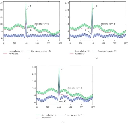
Figure1: Construction of the corrected spectra using a signal,s(x)=180 exp(−0.01(400−x)2) with underlying harmonic components h0 =60.0,h1(x)=10 sin(x/2),h2(x)=10 cos(x/40),h3(x)=25 sin(x/200), so that f(x)=s(x) +h1(x) +h2(x) +h3(x). The spectra are labelled S and the corrected spectra with baseline removal are labelled B; (a)σ=10, (b)σ=100, (c)σ=1000.
which is perturbed by sinusoidally oscillating data sampled from three characteristic frequencies, sin(x/2), cos(x/40), and sin(x/200). All of the baseline curves are produced with a cutoffof 98%. The baselines are generated at values of sigma ranging from 10, 100, and 1000 in Figures1(a),1(b), and
1(c), respectively. It is obvious that whenσ is small, all of the harmonics, except the highest frequency associated with sin(x/2), are well approximated by the baseline curve. Asσ increases, the ability of the curve to respond to the high fre-quencies is diminished, such that whenσ =1000, only the lowest harmonic at sin(x/200) is revealed in the trace of the baseline.
The algorithm produces a succession of baseline curves
B0,B1,. . .,Bm which appear to approach a lower-bound
curveBfor each value ofσ. This curve has the property that it is a baseline curve (it is a Bernstein approximation and thus is infinitely smooth) and it lies below all other baseline curves with p < m. It is not strictly a lower bound to the data, since at somexk the values of yk will exceed the value of the baselineBp(xk). This can be seen in all three plots in
Figure 1where there are a few places where the spectral data undershoot the baseline curve by a small amount. Equally, it is not the greatest lower bound to the data, although it approaches this whenσ is very small, as seen in the graph inFigure 1(a).
combined easily to produce interpolation and deconvolution of the same data, and to do all of these locally through mod-ifications of the structural form of the smoothing by work-ing with σ(x). Since the baseline curves are uniformly ap-proximating, they are well behaved. Moreover, under suitable circumstance, it is possible to construct the baseline curve in one iteration, that is, by constructing only one approxi-mantKnto the data, and we discuss this in greater detail in
Section 6.
4. ENGINEERING PRESENTATION
The new method of baseline drift removal is an iterative ap-proach that repeatedly applies the SB approximation. The in-put signal for the next iteration stage becomes the minimum of the input signal for the current iteration stage and its SB approximation.
An engineering or computer science presentation of the stochastic Bernstein function method is complementary to the mathematical treatment ofSection 3. It offers an appre-ciation for the generality and flexibility of the SB approxi-mation method. The stochastic Bernstein function method (embedded in the iterative process) can be described by pseu-docode as follows.
(1) Read the MALDI-TOF data{(xi,yi)},i=0,n−1 (xi are them/zspectral bins andyiare the spectral inten-sities).
(2) Convert data coordinates to lie on the unit interval. (3) Construct the convolution matrixAnn, which depends
on the data coordinates xi and on the value of the smoothing parameter σ. The generator of the row space ofAnnis a Bernstein function.
(4) Construct the deconvolution matrix,A−1 nn.
(5) Construct the augmented matrixAmn, wherem > n, using the same generator of the row space.
(6) Evaluate AmnA−1
nnz, to obtain output data {zi}, i =
0,m−1.
(7) Convert the output data to the world coordinate sys-tem to obtain the Bernstein function values at the lo-cations of the output data.
These matrices correspond to the mathematical terms al-ready presented. Note also that both the input and the output data points can be nonuniformly distributed inx, and that they can be unrelated to one another, and are of different size (different number of points).
The pseudocode is for the “interpolation” version of the stochastic Bernstein function method. In this version, the Bernstein function passes exactly through the input data points. The “pseudointerpolation” version of the SB method retains all steps but obtainsA−1
nn as an approximate inverse
and causes the Bernstein function to pass very closely but not exactly through the input data points; with the deviation being larger, the more the data deviates from being locally smooth.
The method applied in this paper is the SB “approxima-tion” version of the method. The Bernstein function does not
pass through the input data points. The approximation ver-sion of SB does not require steps 3 and 4 of the pseudocode and also replacesA−1
nnin step 6 by the identity matrix.
5. RESULTS OF APPLICATION AND ILLUSTRATIONS
The process of finding a baseline curve to the proteomics MALDI spectral data as provided through [5] is illustrated inFigure 2. In this case, the spectral data (labelled S) along with the corrected spectral data (labelled C) is shown for two different values ofσ(x). Choosing small σ = 100 re-sults in a limiting baseline curve which still preserves the un-derlying low-frequency oscillation apparent in the spectral data around the spectral peaks atx =5000 andx = 8500. Choosing σ = 10000, however, results in a significantly smoother limiting baseline curve which yields a corrected spectral curve which is significantly flatter and which is lack-ing in any of the low-frequency response which characterizes the data inFigure 2(a). Note also that the limiting baseline curve was attained in about 20 iterations, and that there are still a few points, particularly in the range from 3000 to 7000, where corrected data still have negative values. Clearly, it may be desirable to iterate further to eliminate these negative de-viations, which can be done, however this exceeds the pur-poses of this demonstration.
A more detailed examination of Figure 2 is shown in
Figure 3and it shows that there is no loss in the peak spectral information. The baseline curve does not reduce the magni-tude of the spectral peaks. The use of maximal smoothing, for example, can be seen to provide a spectral curve which is shifted down by 4000 units at the peak atx=5000, however the magnitude of the peaks remains unchanged before and after the baseline correction. This is because the SB approxi-mation forσ 1 does not respond to high-frequency oscil-lations and thus is acting as a lowpass filter only. Note that us-ing a smaller value of the parameterσ(using strong smooth-ing) causes even the lower-frequency hump fromx = 4000 tox =6000 to be ignored in the generation of the baseline curve, and thus causes the hump to be incorporated into the spectral data. In comparison, using a larger value forσallows the SB approximation to pick up the low-frequency values along the hump, yielding a baseline curve which contains this low-frequency oscillation, thus resulting in a spectral curve which is flatter as shown inFigure 3(a).
Although MALDI-TOF is found principally in pro-teomics, it is also used in genomics.Figure 4gives an overall appreciation for the baseline correction for a spectra of ge-nomics origin.Figure 5illustrates the sensitivity to the value ofσ(x) on this particular data. In these experiments, the sen-sitivity is not great but in other cases of baseline correction it would be necessary to optimizeσ(x).
5.1. Remarks
0 5000 10000 15000 20000 25000 30000 35000 40000
−2 0 2 4 6 8 10 12 14 16 18×10
3
S
C
Spectral data (S) Midline approximation
Baseline curve
Spectra corrected for baseline (C) (a)
0 5000 10000 15000 20000 25000 30000 35000 40000
−2 0 2 4 6 8 10 12 14 16 18×10
3
S C
Spectral data (S) Midline approximation
Baseline curve
Spectra corrected for baseline (C) (b)
Figure2: Convergence of SB approximation to 15 000 data point spectra applying min-mean baseline algorithm. (a) The approximations are computed using minimal smoothing as this removes the baseline hump atx=5000 andx=8500. (b) The approximations are computed using strong smoothing as this preserves the baseline hump atx=5000 andx=8500.
4600 4800 5000 5200 5400 5600 5800 6000 0
2 4 6 8 10 12 14 16 18×
103
S
M C
B
Spectral data (S)
Midline approximation (M) Baseline curve (B)
Spectra corrected for baseline (C) (a)
4600 4800 5000 5200 5400 5600 5800 6000 0
2 4 6 8 10 12 14 16 18×
103
S
M
C
B
Spectral data (S)
Midline approximation (M) Baseline curve (B)
Spectra corrected for baseline (C) (b)
Figure3: Detail fromx=4500 to 6000 for the min-mean baseline corrected spectra shown inFigure 2. The approximations inFigure 3(a) are computed using minimal smoothing and inFigure 3(b)are computed using strong smoothing.
distortion of the signal by the method. Inevitably, every numerical method affects the signal in some manner. A com-pelling reason for choosing the SB approximation in de-veloping this method, aside from the algorithmic simplic-ity of the approach, is that it does not introduce any false
1000 2000 3000 4000 5000 6000 7000 8000 9000 10000
−2 0 2 4 6 8 10 12×10
2
S
C
Spectral data (S) Corrected spectra (C)
Figure4: Original and baseline corrected MALDI-TOF spectra us-ing the method withσ=150.
this property cannot be attained without the introduction of limiters to prevent overshooting and undershooting be-tween interpolation points. Furthermore, unlike other poly-nomial approximation methods, the SB approximation can be constructed for even a large number of points in the computational stencil, and unlike the Bernstein polynomials to which the Bernstein functions are related, the properties can be tuned to increase or decrease the smoothing through the choice of the parameterσ and if required to determine this choice with evolutionary computation, for example, ge-netic programming. This provides control and efficiency.
The efficiency of the algorithm can be increased signifi-cantly by computing a baseline correction over sets of data: by restricting the range of the summation in the computa-tional stencil for each output point. Since for baseline cor-rection, each output data pointxkis located at the samex -coordinate as the input value, the sum in the SB approxima-tion can be taken over the rangek−ntok+n, wherenis sufficiently large to ensure that the tail of the sum is insignif-icant. Forσ on the order of about 100, this means including only several hundred values on either side of the output point into the sum. Clearly, this saves significantly with data sets as large as in the example being considered. In these examples, the sums were computed using a truncated sum. In addition, the costly computation of erf(u) for each value ofuin the sum was done only once, and saved to an array, so that for all subsequent computations ofKn, the values were reused. In computing the baseline curves Bj, j > 0, the operation consisted of a short-matrix-vector multiply, which isO(n2).
6. FINDING THE BASELINE DIRECTLY
The approach described thus far for finding the baseline is an iterative method, requiring the computation of successive
2700 2705 2710 2715 2720 2725 2730 2735 2740 2745 2750
σ=1.5
σ=150, 1500 S
−1 0 1 2 3 4 5 6 7 8×10
2
Spectral data Correctedσ=150
Correctedσ=1500 Correctedσ=1.5
Figure5: Detail fromx =2700 to 2751 for the baseline corrected spectra shown inFigure 4, showing SB approximation baseline cor-rected MALDI-TOF using two different values of the parameter σ(x). One of the curves usesσ=150 and the other usesσ =1500. Note in this case that both methods perform similarly.
approximations to the data setsDkas described inSection 3. The convergence rate to a usable baseline depends on the spectral content of the data, as well as whetherσis large or small. Typically, it requires anywhere from 10 to up to 100 iterations to find the baseline, and this does not include the effort required to evaluate the baseline using different val-ues of σ. Clearly, the fundamental approach we have de-scribed is usable, however in implementing this approach with the more sophisticated functional representational tech-niques, including pseudointerpolation and windowing com-bined with adaptive, intelligent algorithms, would require that many baselines be iteratively constructed.
In many cases, it is possible to construct the baseline di-rectly. The reason is that in most cases, the midline approx-imation provided by the first iterationB0is nearly a shifted copy of the baseline curve. Evidently, this is not always the case, and it is possible to devise spectral data which would cause this approach to break down; however for many of the spectral data examined, this approach provides a quick es-timate, and thus can be used in these cases to more rapidly characterize the baseline.
The alternative consists of finding the midline curve, and subtracting this from the data. This removes all of the long-wave oscillations, if we add back the minimum value of this curve, we would get a spectrum which has been straight-ened out, more or less, depending on the value of sigma. The resulting baseline curve is not computed. The values of
σat which we get the same results as computing the baseline curve iteratively would be different, since in the iterative case, smoothing is applied to a partially smoothed data set at each step.
4800 4900 5000 5100 5200 5300 S
B C
0 2 4 6 8 10 12 14 16 18
×103
Spectral data (S) Baseline (B) Corrected spectra (C)
(a)
4800 4900 5000 5100 5200 5300
0 2 4 6 8 10 12 14 16 18
×103
S
B C
Spectral data (S) Baseline (B) Corrected spectra (C)
(b)
Figure6: Convergence of the min-mean baseline algorithm (a) using minimal smoothing,σ = 0.1, and (b) using strong smoothing, σ=100.0. The spectra are taken from the same data set as shown inFigure 2.
4800 4900 5000 5100 5200 5300
S
B C
0 2 4 6 8 10 12 14 16 18
×103
Spectral data (S) Baseline (B) Corrected spectra (C)
(a)
4800 4900 5000 5100 5200 5300
0 2 4 6 8 10 12 14 16 18
×103
S
B C
Spectral data (S) Baseline (B) Corrected spectra (C)
(b)
results shown inFigure 7for the corrected spectra obtained by using a direct approach. For either case of weak or strong smoothing, the corrected spectra appear very similar, and in-deed overlaying these on the same graph would show only negligible differences.
7. CONCLUSIONS AND FUTURE WORK
The application of stochastic Bernstein function approxima-tion can be seen to produce usable families of baseline curves for correcting spectral data bias shift due to low-frequency errors. There are several advantages to this approach, most notably its algorithmic simplicity and robustness. Unlike methods based on interpolation of various means, there is no possibility of any instabilities arising due to the interpolation process, and thus no possibility of generating any spurious oscillations which may affect the signal.
Perhaps the most useful feature of this approach is that the computations can be incorporated into many adaptive algorithms in which the value ofσ is optimized with regard to several selection criteria. For constantσ, tuning is simple. More sophisticated analysis may use genetic programming [7] to evolve polynomial terms for the functionσ(x).
This offers further research opportunities. Is it worth-while revisiting research that obtains candidate biomarkers and a sample classification from MALDI-TOF data (e.g., [8]) to investigate the sensitivity of results to different amounts of baseline drift removal? Can tuning clarify the nature of chemical noise in different conditions (Section 2)? Finally, by means of supervised-learning, it should be possible to fine tune baseline drift removal for different instrumentation.
The SB method [1] was recently combined with genetic programming [9] and this opportunity is immediately avail-able for problems of baseline drift.
In attempting to optimize the baseline, the use of the di-rect method for computing the baseline has obvious advan-tages, and it should be tried before anything else. At worst, it may be necessary to construct it iteratively.
ACKNOWLEDGMENTS
We are grateful to Sequenom Corporation of San Diego, for providing us with MALDI-TOF genomics data. We are also indebted to Professor Franz Hillenkamp from the Insti-tute for Medical Physics and Biophysics at the University of M¨unster in Germany for furnishing us with the information that is presented inSection 2of this paper.
REFERENCES
[1] J. Kolibal and C. Saltiel, “Data regularization using stochastic methods,” 2005, to appear inSIAM Journal on Numerical Anal-ysis,Paper ID is: Manuscript # 063083.
[2] M. Karas and F. Hillenkamp, “Laser desorption ionization of proteins with molecular masses exceeding 10,000 daltons,” An-alytical Chemistry, vol. 60, no. 20, pp. 2299–2301, 1988. [3] M. A. Ryan, M. G. Buehler, M. L. Horner, et al.,Results from the
space shuttle STS-95 electronic nose experiment, JPL Publication 99-0780, 1999.
[4] G. G. Lorentz,Bernstein Polynomials, Chelsea, New Yourk, NY, USA, 1986.
[5] B. Williams, S. Cornett, A. Crecelius, R. Caprioli, B. Dawant, and B. Bodenheimer, “An algorithm for baseline correction of MALDI mass spectra,” inProceedings of the 43rd ACM Southeast Conference (ACMSE ’05), Kennesaw, Ga, USA, March 2005. [6] A. N. Krutchinsky and B. T. Chait, “On the nature of the
chem-ical noise in MALDI mass spectra,”Journal of American Society of Mass Spectrometry, vol. 13, pp. 129–134, 2002.
[7] J. R. Koza,Genetic Programming, MIT Press, Cambridge, Mass, USA, 1992.
[8] H. W. Ressom, R. S. Varghese, E. Orvisky, et al., “Analysis of MALDI-TOF serum profiles for biomarker selection and sam-ple classification,” inProceedings of IEEE Symposium on Com-putational Intelligence in Bioinformatics and ComCom-putational Bi-ology (CIBCB ’05), San Diego, Calif, USA, November 2005. [9] D. Howard and J. Kolibal, “Solution of Differential Equations
with Genetic Programming and the Stochastic Bernstein Inter-polation,” Tech. Rep. BDS-TR-2005-001, Biocomputing Devel-opmental Systems Group, University of Limerick, Limerick, Ire-land, June 2005.
Joseph Kolibal received a B.S. degree in chemical engineering from Carnegie Mel-lon University, an M.S. degree in nuclear engineering from Imperial College, and his D.Phil. degree in numerical analysis from Oxford University. He joined the Mathe-matics faculty of the University of Southern Mississippi (USM) where he is a Tenured Associate Professor. In 2005 at USM, he de-veloped methods for stochastic Bernstein
approximation and interpolation. His research is focused on func-tional approximation, partial differential equations, and numerical analysis.
Daniel Howard received a B.S. degree in chemical engineering from Lafayette Col-lege, an M.S. degree in chemical engineer-ing from Swansea University, and his Ph.D. degree from the Civil Engineering Depart-ment of Swansea University. He is a for-mer Research Fellow of Pembroke College and the Numerical Analysis Group of Ox-ford University. Employed at QinetiQ in the United Kingdom (the former Defence