Mobile Robot Visual Navigation Using Multiple Features

(1)

Mobile Robot Visual Navigation Using

Multiple Features

Nick Pears

Department of Computer Science, University of York, York Y010 5DD, UK Email:[email protected]

Bojian Liang

Zezhi Chen

Received 22 December 2003; Revised 29 July 2004

We propose a method to segment the ground plane from a mobile robot’s visual field of view and then measure the height of nonground plane features above the mobile robot’s ground plane. Thus a mobile robot can determine what it can drive over, what it can drive under, and what it needs to manoeuvre around. In addition to obstacle avoidance, this data could also be used for localisation and map building. All of this is possible from an uncalibrated camera (raw pixel coordinates only), but is restricted to (near) pure translation motion of the camera. The main contributions are (i) a novel reciprocal-polar (RP) image rectification, (ii) ground plane segmentation by sinusoidal model fitting in RP-space, (iii) a novel projective construction for measuring aﬃne height, and (iv) an algorithm that can make use of a variety of visual features and therefore operate in a wide variety of visual environments.

Keywords and phrases:plane segmentation, image rectification, plane and parallax, obstacle detection, mobile robots.

1. INTRODUCTION

1.1. Robust, multifeature, multicue vision systems In order to operate reliably over extended periods of time (i.e., hours/days/weeks rather than seconds/minutes), com-puter vision systems must use of all the information in the image stream that is pertinent to the current task. This re-quires that the system can make this pertinent information explicit by employing a range of feature extractors and visual cues opportunistically, namely, as and when they are avail-able in the image stream and deemed to provide useful con-straints to solve task-related problems and resolve any ambi-guities. In this way, visual interpretation and decision making can be maximally informed.

We believe that this principle is particularly important in unconstrained environments when the visual environ-ment regularly changes because the disambiguating infor-mation content in the image stream is continually chang-ing. Thus if we rely on a single feature/cue combination, such as corners/corner-motion, the application will fail in scenes with few corners, or poorly distributed corners in im-age space.

We have focused on mobile robot visual navigation as a challenging computer vision problem because the nature of the application suggests that the visual environment is likely to be variable as the robot moves, for example, from room to room. Indeed, we make no assumptions in the work pre-sented here, other than having a reasonably flat floor. This makes the work applicable to mainly indoor mobile robot ap-plications, but also outdoor applications which traverse rea-sonably flat man-made structures such as pedestrian walk-ways.

(2)

planar region detection using point correspondences [12]. Most of these techniques work in some types of scene, but will fail when a particular type of feature/cue combination is not well supported within the image data. We believe the solution is to employ multifeature, multicue approaches.

A point to note is that systems that use this multifea-ture, multicue philosophy will be highly compute-intensive, due to having a range of processes with a high-bandwidth data input (raw video data). We envisage that the high-bandwidth low-level feature extractors will be implemented as a hardware layer with parallel processing pipelines, either via field-programmable gate arrays (FPGAs) or special pur-pose DSPs, which output a feature stream. Higher-level layers of software will be able to access the much lower-bandwidth feature stream and select/combine/fuse those parts of the stream, thus providing information or constraints relevant to the particular visual task (in our case robot navigation). Of course, how best to design a framework that allows a computer vision system to understand how to combine fea-tures and cues in the context of the current visually-driven task and in the context of the current visual environment is a diﬃcult, open, cross-disciplinary research question. What we aim to do is less ambitious: we aim to develop computer vision applications that are robust, because they are able to make use of multiple features/cues. There is no explicit scene understanding as such, but we need to understand how to build multifeature, multicue algorithms manually before we can develop systems that learn and adapt the way in which they integrate features and cues.

The algorithm that we describe in the following section is able to provide (i) the segmentation of the ground plane or, equivalently, grouping of the ground plane pixels, (ii) a mea-surement of the height of all other features (corners, edges, or even pixels) above the extracted ground plane. Obviously, such information may be fed directly into a range of obstacle avoidance algorithms (both behavioral and planned path), but may also be used as an input into robot localisation and mapping algorithms.

The algorithm can make use of ground plane and non-ground plane corner features, but if those are scarce (we need at least two corner correspondences), it can make use of any region that has some local intensity variation. If there is no local intensity variation (i.e., if the region is smooth), it can make use of the motion/deformation of the boundary of the smooth region, where boundaries are extracted using a seg-mentation algorithm based on color-texture properties.

1.2. Outline of a multifeature, multicue robot visual navigation

In this paper, we focus on the application of mobile robot (uncalibrated, monocular) obstacle avoidance and we present a system that can construct an affine height landscape of the robots visible (indoor) environment. The height re-covered is termed anaffine heightas it is a height ratio (affine invariant property) referenced to the height of the camera optical center above the ground plane or alternatively some known height measurement in the scene. The termlandscape

is used as the other two dimensions are view-based (i.e., un-transformed pixel coordinates). Aﬃne height (ha) measure-ments allow potential obstacles to be classified as either small enough to be driven over (we requireha<0.1), high enough to be driven under (we requireha >1.25), or true obstacles to be avoided.

There are several different methods to determine scene structure in the computer vision literature. For example, 3D world structure can be computed from uncalibrated views of a scene given sufficient correspondences in general posi-tion and this has already been used to answer specific, met-ric questions about the scene. The approach by Tomasi and Kanade [8] is known as the factorization method; Triggs [9] extends the factorization method to the projective camera model by using epipolar constraints to calculate depth scale factors; Heyden et al. [11] upgrade the affine approximations to projective results by iterative optimization. Others use the camera-centered approach where the first view is used as the reference camera to determine the projection matrices of other cameras in a projective frame under multiple view geo-metric constraints. Criminisi et al. [6] proposed methods to make measurements of world planes from their (single) per-spective images. Reid and Zisserman [4] give a method for locating 3D position of a soccer ball from monocular image sequence of soccer games.

An important part of our algorithm is that it can use a wide range of features, but, in addition, we present three significant new results: first, by expressing images in a reciprocal-polar (1/r,α) form with the origin on the focus of expansion (FOE),1_{the image motion of a set of coplanar} points along the 1/rdirection is a pure shift, when the trans-lation is parallel to the plane. This allows image motion to be accurately recovered by 1D correlation, even over large im-age distortions caused by large camera motion. Second, we show that the magnitude of these shifts follows a sinusoidal form along the αdirection over a maximum of π radians. Simultaneous ground plane pixel grouping and recovery of the ground plane homography thus amounts to finding the FOE and then robustly fitting a sinusoid, whose phase corre-sponds to the orientation of the vanishing line of the ground plane and whose amplitude is related to the magnitude of the robot/camera translation. The method allows every ground plane pixel in a locally textured region to contribute to the estimation of the ground plane homography, thus giving a highly accurate result. Finally, our third new result shows that given the homography associated with the ground plane, the aﬃne height of remaining nonground plane pixels, refer-enced to the height of the camera optical center above the ground plane, can be determined using the virtual parallax cue computed using a construction based on the cross-ratio. Our algorithms require camera motion that is (near) pure translation. Obviously, it can be argued that this is re-strictive, but such motions are common, can be deliberate

(3)

in mobile robot applications, and can easily be detected over an image pair, particularly when corner correspondences are available. Also, given that an aﬃne height landscape has been computed, it can be tracked through robot motions which have a rotational component, and new unlabelled areas of the scene that enter the field of view can be probed by fur-ther translation motions.

In the following sections, we first discuss ground plane motion (and hence homography) recovery, which simultane-ously gives a ground plane segmentation. We then show how the recovered homography can be used to measure aﬃne height.

2. GROUND PLANE SEGMENTATION AND GROUND

PLANE MOTION/HOMOGRAPHY RECOVERY Early work on exploiting coplanar relations has been pre-sented by Tsai and Huang [1], Longuet-Higgins [7], and Faugeras and Lustman [10]. We summarise the coplanar re-lation as follows: if a set of feature points in the scene lie in a plane, and they are imaged from two viewpoints, then the corresponding points in the two images are related by a pla-nar homography,H, such thatλxj=Hxi, wherexrepresents a homogenous image coordinate (x,y, 1)T_,_H_{is a 3}_×₃ ma-trix representing the homography, andλis a scalar. Since this equation is valid up to a scale factor,Hhas only eight degrees of freedom.

Suppose that a mobile robot (and therefore camera) at-tempts to move under pure translation. Due to an uneven floor surface and hysteresis in the robot’s mechanics, the mo-tion is unlikely to be pure translamo-tion. However, if rotamo-tion is relatively small with respect to the translation, assuming pure translation and enforcing a homography correspond-ing to pure translation allows correlation-based techniques to be used. The key point here is that this allowsallground plane pixels which have local intensity/color variation to be used in the simultaneous estimation of the ground plane ho-mography and grouping of ground plane pixels.

Under pure translation, not necessarily parallel to the plane, a planar homography is often termed a planar homol-ogy [16], which has five degrees of freedom (dof) and takes the form

H=I−kxflTv, (1)

wherexf =[xf,yf, 1]T is the focus of expansion (FOE) for the two frames,lv=[av,bv, 1]Tis the vanishing line (or hori-zon line) of the plane, andkis a constant associated with the magnitude of the translation.

Firstly, we check if (near) pure translation is detected, by intersecting all lines defined by all corner correspon-dences from the image pair. If most lie in a small area (95% of intersections should lie within a circle of small radius), then translation is assumed and the FOE is computed us-ing random sample consensus (RANSAC [13]) and least squares (LS). Once the FOE has been computed, we shift im-age coordinates so that each imim-age is centered on the FOE.

Thus we apply the centering translationTcwhere

Tc=

  

1 0 −xf 0 1 −yf 0 0 1

 

. (2)

After this translation, the FOE is at homogenous coordinates x_f =[0, 0, 1]T_{and the vanishing line becomes}_l

v=T−cTlv= [av,bv,xTflv]T. Thus, the homography relating points in FOE centered coordinates isH=I−kx_flT

v , and substituting this in the equationλx₂=Hx1and expanding gives

λ

  

x2

y2 1   =   

1 0 0

0 1 0

−kav −kbv (1−kq)      

x1

y1 1  

, (3)

whereq =xT

flv. We note that for translation parallel to the ground plane,q=0 since the FOE lies on the vanishing line. In this specialisation, the homography has four dof and is sometimes called an elation [16]. Otherwise, the FOE is at a distanced=q/a2

v+b2vfrom the vanishing line. To simplify notation, we now drop the “prime” notation from (3) and assume that (x,y) are image measurements made relative to the FOE. Thus, we have

−kavx1−kbvy1+ 1−kq x2=x1,

−kavx1−kbvy1+ 1−kq y2=y1.

(4)

Squaring both sides and adding,

−kavx1+bvy1 + (1−kq) 2

x2

2+y22 =

x2

1+y12 . (5) If we define ri as the Euclidean distance between an image point and the FOE in framei, then, taking square roots of (5),

−kavx1+bvy1 + (1−kq) r2=r1,

r−1 2 = −k

avx1+bvy1 r1−1+ (1−kq)r1−1,

r−1 2 = −k

avcosα+bvsinα + (1−kq)r1−1, (6)

whereαis the angular position of a pixel in a frame centered on the FOE. Now the gradient of the vanishing line is given as tanαv= −av/bv, so

av= −

a2

v+b2v sinαv, bv=

a2

v+b2v cosαv. (7) Hence

r2−1=kp

−sinαvcosα+ cosαvsinα +kqr1−1, (8)

where

(4)

Hence, we arrive at the key equation which defines a function of the angleα,s(α), as

s(α)=ρ2−kqρ1=kpsin

α−αv , (10)

where we define ρ = 1/r. Equation (10) indicates that we need to find three constants (kq,kp,αv) in order to recover the homography and that the computation should be imple-mented in (ρ,α) image space. (Note that a planar homology has five dof, but two have been recovered in the FOE com-putation.) We callI(ρ,α) reciprocal-polar (RP) image space. Thus, after computing the FOE, an interpolation procedure is used to generate a (possibly scaled) RP image for each im-age in the imim-age pair.

For the set of planes parallel to the translation direction (which includes the ground plane), the expected value ofkq will be unity, as the expected value ofqis zero. For certain applications (hard flat floor, hard robot wheels), it may be reasonable to assume kq is unity,as we do. In other appli-cations, it may be preferable to estimate this value, although any estimated value is likely to be very close to unity. For each pixel in image 1, its position in RP image space is computed, and a 1D window is created around this position along the

ρdimension. We then correlate this window along theρ di-mension in RP image 2, at the same value of α. The posi-tion of the maximum value of the correlaposi-tion is retained as a value ofsi(α). Equation (10) indicates an important result: coplanar motions in RP image space lie on a sinusoid and the constants(kp,αv)may be recovered by fitting a sinusoid to the RP motion data,s(α). Suppose that we have two values ofs,

si,jmeasured at two angles,αi,j, so that

si=kpsin

αi−αv , sj=kpsin

αj−αv , (11)

hence

si

sj =

sinαicosαv−cosαisinαv sinαjcosαv−cosαjsinαv ,

si

sj =

sinαi−cosαitanαv sinαj−cosαjtanαv.

(12)

Collecting terms in tanαvand rearranging gives

tanαv= sj

sinαi−sisinαj

sjcosαi−sicosαj.

(13)

Thus a pair ofsvalues, at diﬀerent angular positions, for

pix-els belonging to the same plane, allows us to estimate the ori-entation of the vanishing line of that plane. Given the phase angle,αv, corresponding to the orientation of the vanishing line, we can computekpfrom (11). By selecting random pairs of anglesαi,jand computing the associated magnitude and phase of the sinusoid upon which bothsiandsjlie, a random sample consensus (RANSAC) procedure [13] can be used to determine the best set of inliers in thes(α) data to a puta-tive sinusoid. This putaputa-tive sinusoid is used to initialise an

iterative procedure where an LS estimate of the sinusoid pa-rameters and the associated set of inliers are computed un-til the inlier distribution, represented by a binary tag string, stabilises or the maximum number of iterations is reached. In this way, coplanar pixels may be grouped without explicit construction of a homography matrix. Now, let

si=kpsin

αi−αv =msinαi−ncosαi, (14)

wherem=kpcosαv = −kbv,n=kpsinαv = −kav. Thus, for the inliers of the sinusoid model, we can write



−sin_.. αi cosαi si . ... ...     mn

1  

=0. (15)

We use singular value decomposition (SVD) to solve for

λ[m,n, 1]T_{and normalise the solution to obtain the} parame-ters, (m,n). From (3), we substituten = −kav,m= −kbv, and kq = 1−kq, to recover the homography in an FOE centered frame. The parameters defining s(α) can be com-puted askp =

(m2₊_n2_), _α

v =tan−1(−n/m) and the ho-mography in the original image frames can be computed as

H=T−1

c HTc.

How do we know that the recovered homography and grouped pixels are associated with the ground plane? A weak assumption regarding the pose of the camera with respect to the ground plane suggests that the sinusoid phase should be close to zero (near horizontal vanishing line). Also, since translation is roughly parallel to this plane, the FOE should lie very close to the vanishing line.

To test whether we can recover the sinusoidal model sug-gested by the analysis,kq = 1 was assumed and two frames were captured before and after the robot moved in the trans-lation mode. The images were then converted using an inter-polation process (this may be a simple linear interinter-polation or based on cubic splines) to RP (ρ,α) form.Figure 1ashows one of the original images which has its FOE sixteen pixels above the top center edge of its image. Its RP transform is in

Figure 1b and shows the angular (α) axis and lines of con-stant (reciprocal) radius in the vertical direction. The axis representing (scaled) reciprocal distance from the FOE (ρ) and reciprocal radial lines (constant angle) are in the hori-zontal direction. For a more intuitive viewing, the horihori-zontal rendering of the RP image is such thatr increases from left to right, thus ρincreases from right to left. In this render-ing of the RP image, the FOE is out at infinity to the left of the image. In order to usefully constrain the size of the RP image, any pixels less than 64 pixels from the FOE are not in-cluded in the RP plot. In any case, the motion near the FOE is so small that it is not possible to make accurate height mea-surements in this image region. In terms of implementation details, we used VGA-sized images (640×480) as the raw in-put images and we generated RP images such that there was no information loss due to pixel compression.

(5)

(a) (b)

Figure1: (a) shows an original imageI(x,y) and (b) shows the corresponding RP imageI(ρ,α).

value by correlating along a line of constantα(i.e., horizon-tally) in the first RP image of the pair. (We map the second to the first rather than vice versa, due to field of view con-siderations.) The maximum value of correlation is retained as a value for s(α). A correlation window size of 64 pixels was used in the RP image, with a search window of 150 pix-els. Due to the high-frequency repetitive structure of the car-pet microtexture shown inFigure 1a, often many local max-ima are generated in the correlation process. However, due to low-frequency components of spatial frequency, the global maximum, in most cases, corresponds to the correct image motion that we wish to recover. Even if this is not the case, it is possible to include pixels with significant local maxima, if these strong local maxima are consistent with the extracted planar motion, that is, they lie suﬃciently close to the ex-tracted sinusoid model.

The plot ofs(α) againstαis shown inFigure 2a for all pixels. Those pixels motions that correspond to the ground plane can clearly be seen to lie on a sinusoid and ground plane pixels can be segmented as inliers to this sinusoid and used to compute the ground plane homography. The inliers of the recovered sinusoid are then plotted in 3D in

Figure 2b, with the third dimension representingρ. This in-dicates that the same sinusoidal form captures image motion in RP-space, irrespective of a pixel’s distance from the FOE, as expected.

3. AFFINE HEIGHT MEASUREMENT

The approach described above allows pixels to be classified as either belonging to the ground plane or not. For those non-ground plane regions, we would like to know whether we can drive over/under them or whether they form part of an ob-stacle which should be avoided. We now develop a method of aﬃne height measurement referenced to the height of the camera optical center above the ground plane.

Our aim is to recover the height of feature pointAshown inFigure 3when the robot undergoes pure (forward) trans-lation,t(and thus the scene point translatestunits towards the robot). PointAis the actual position of the feature point

relative to the camera before the translation and pointCis the position of the feature after the translation. Points A

andCare the projections of these actual feature positions onto the ground plane. Points aandcare the image posi-tions of the feature at posiposi-tionsA andC, respectively, and

bis the predicted image position of the feature point, if the feature point were to lie in the ground plane. Image pointb

is computed from the recovered homography induced by the ground plane asb=Ha. Referring toFigure 3, the height of the feature point relative to the height of the camera optical center, the aﬃne height, is

ha= h

hc = 1−D

hc.

(16)

Using similar triangles, and denoting the distance between pointsxandyasd(x,y), we note that

D hc =

d(OC)

d(OC₎=

d(AC)

d(A_C₎. (17)

For pure translation,d(A,C)=d(A,B), so that

ha=1−d(A

_B₎

d(A_C₎. (18)

Now, the four image points (a,b,c,xf), wherexf is the fo-cus of expansion (FOE), and the corresponding four ground plane points (A,B,C,∞) are collinear. The cross-ratio for this set of points remains invariant under projection and so we can write

d(AB)

d(A_,_C₎=

d(a,b)dc,xf

d(a,c)db,xf .

(19)

Hence, for features below the vanishing line, we can compute aﬃne height as

ha=1−

d(a,b)dc,xf

d(a,c)db,xf .

(6)

0 50 100 150 200 θ(deg)

0 50 100 150

f

(

θ

)

(a)

200

100

0 0

2000

4000

6000 θ(deg)

ρ(scaled) 0

50 100 150

f

(

θ

)

(b)

Figure2: (a) All image motion in RP-space. (b) Ground plane image motion in RP-space withρplotted explicitly.

Ground plane C B t A

h hc

D

C

t A Optical axis O Image plane

xf

a b c

Figure3: Measuring the height of pointA.

In general, we find that

ha=1 +µd

(a,b)dc,xf

d(a,c)db,xf

, (21)

where µ = −1 for features below the vanishing line and

µ = +1 for features above the vanishing line. (Obviously

ha = 1 for features on the vanishing line.) This can be in-terpreted as the height of pointAin units of heighthc. Note that this approach only needs the ground plane homography,

H, and the image correspondencesaandcof the feature to determine the height above the ground plane. By threshold-ing the measured height above the plane, the method can be used to check for areas which can be driven over, and for suf-ficiently high features, which can be driven under. Note that this is achieved without camera calibration.

4. EXPERIMENTAL RESULTS

4.1. Ground plane segmentation by ground plane pixel grouping

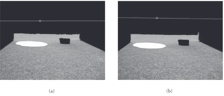
In the two experiments shown inFigure 4, the ground plane was segmented on a pixel-by-pixel basis, as the robot trans-lated forwards. Those pixels that fit the ground plane sinu-soid in RP image space are retained and plotted as ground plane pixels, all other pixels are removed from the image (rendered as zero intensity, or black). Comparing the seg-mentations with their original images, it can be seen that the pixel-by-pixel grouping gives an accurate ground plane seg-mentation. For example, the small, black door stop on the center-right of the first sequence is clearly and correctly ex-cluded. Also, the small piece of carpet at the foot of the door in the center-left of the second sequence is clearly and cor-rectly included. Note also that the extracted FOE is shown as a small circle in both sequences and the vanishing line of the ground plane, whose orientation is extracted as the phase of the RP sinusoid is also shown as a near horizontal line (near zero sinusoid phase).

4.2. Height measurement experiments

(7)

(a) (b)

Figure4: Image sequences showing ground plane segmentation. (a) Image sequence 1. (b) Image sequence 2.

we computed tanαv= −0.03. Results are shown inFigure 5 and inTable 1, where “TM” are the manual (tape measure) measurements and “VM” are the results from our automatic height measurement method. We find a mean absolute error of 6.9 mm and mean relative error of 0.35%. If we remove the two rather inaccurate measurements (a)EF and (a)PQ, the remaining measurements have a mean absolute error of 1.5 mm and a 0.1% mean relative error.

4.3. Using height profiles of smooth regions to segment the ground plane

The final experiment presented in this paper uses both the si-nusoid fitting process (to simultaneously recover the textured

Table1: Height measurement results in centimetres.

Segment TM VM Segment TM VM

(a)CD 30.0 29.88 (b)CD 233.1 233.08 (a)EF 227.7 229.36 (b)EF 149.8 149.51 (a)LM 208.4 208.23 (b)GH 258.7 258.55 (a)GH 252.5 252.73 (b)MN 233.1 232.67 (a)NO 121.1 120.94 (b)OP 149.8 149.82 (a)PQ 210.3 214.91 (b)QR None 651.51

(8)

(a) (b)

Figure5: (a) Indoor height measurement experiment, and (b) outdoor height measurement experiment.

(a) (b)

Figure6: (a) Raw image. (b) Boundaries to be matched using recovered FOE.

100 200 300 400 500

Curve length (pixels) 0

0.2 0.4 0.6 0.8 1

H

eig

ht

ra

tio

(a)

50 100 150 200

Curve length (pixels) 0

0.2 0.4 0.6 0.8 1

H

eig

ht

ra

tio

(b)

(9)

(a) (b)

Figure8: Two frames of the extracted ground plane. (a) Height profile of white paper. (b) Height profile of small box.

belong to the ground plane or not. Note that an additional process is required, not described in this paper, which is a quadtree split-merge region segmentation algorithm which extracts homogenous regions of color-texture. Textureless re-gions cannot be classified as ground plane or nonground plane as they cannot be matched across an image pair. Their boundaries, however, can be and, in the case of pure transla-tion, this is easily done by casting rays from the FOE recov-ered in the homography estimation process.

Figure 6ashows an image with two regions on the floor which have little texture. The first is a circular piece of white paper which can be driven over, and the second is a small cardboard box, which can not.Figure 6bshows the extracted boundaries and the FOE used to cast a ray in order to match intersections between corresponding boundaries. The cross-ratio construct to measure aﬃne height is applied to the cor-respondences, thus allowing a height profile to be extracted as we “walk around” the closed contours associated with the two low-texture regions. If the height profile remains close to zero, then the region can be classified as belonging to the ground plane, as inFigure 7a. Otherwise it is classified as an obstacle, as inFigure 7b. The final image inFigure 8, shows two frames of the extracted ground region where the textured carpet has been classified on a pixel-by-pixel basis, and the textureless white paper region has been included by virtue of the height profile of its boundary. Obviously, this could have been done by determining whether the contour motions in reciprocal-polar space lay close to the extracted sinusoid defining the homography, but this does not give any quan-titative information about height which may be necessary if we wanted to allow the robot to drive over obstacles of small height compared to the robot wheel diameter.

5. CONCLUSIONS

We have described a method which allows a mobile robot’s ground plane to be segmented and an aﬃne height land-scape constructed by probing the environment with trans-lation manoeuvres. A key point is that all ground plane pix-els which have some local variation in intensity/color can be

used to contribute to the ground plane homography compu-tation and also, we can classify the (transformed) image to be ground plane or nonground plane at pixel level. The al-gorithm uses 1D correlations and the robust LS fitting of si-nusoids to the resulting shift data to simultaneously recover the ground plane homography and classify pixels. Results have confirmed the validity of both the sinusoid model ex-traction and aﬃne height measurement procedure. The ap-proach may be used for a range of feature types including corners, edges, region boundaries, and even raw pixels if they have some local color-intensity variation.

REFERENCES

[1] R. Tsai and T. Huang, “Estimating three-dimensional mo-tion parameters of a rigid planar patch,”IEEE Trans. Acoust., Speech, Signal Processing, vol. 29, no. 6, pp. 1147–1152, 1981. [2] D. Coombs, M. Herman, T.-H. Hong, and M. Nashman,

“Real-time obstacle avoidance using central flow divergence, and peripheral flow,”IEEE Trans. Robot. Automat., vol. 14, no. 1, pp. 49–59, 1998.

[3] J. Santos-Victor, G. Sandini, F. Curotto, and S. Garibaldi, “Divergent stereo in autonomous navigation: from bees to robots,” International Journal of Computer Vision, vol. 14, no. 2, pp. 159–177, 1995.

[4] I. D. Reid and A. Zisserman, “Goal-directed video metrology,” inProc. European Conference on Computer Vision (ECCV ’96), R. Cipolla and B. Buxton, Eds., vol. 2, pp. 647–658, Cam-bridge, UK, April 1996.

[5] R. Okada, Y. Taniguchi, K. Furukawa, and K. Onoguchi, “Obstacle detection using projective invariant and vanishing lines,” inProc. IEEE 9th International Conference on Computer Vision (ICCV ’03), pp. 330–337, Nice, France, October 2003. [6] A. Criminisi, I. D. Reid, and A. Zisserman, “Single view

metrology,”International Journal of Computer Vision, vol. 40, no. 2, pp. 123–148, 2000.

[7] H. C. Longuet-Higgins, “The reconstruction of a plane sur-face from two perspective projections,”Proceedings of Royal Society of London B, vol. 227, pp. 399–410, 1986.

[8] C. Tomasi and T. Kanade, “Shape and motion from image streams under orthography: a factorisation approach,” Inter-national Journal of Computer Vision, vol. 9, no. 2, pp. 137–154, 1992.

(10)

Computer Vision and Pattern Recognition (CVPR ’96), pp. 845–851, San Francisco, Calif, USA, June 1996.

[10] O. Faugeras and F. Lustman, “Motion and structure from mo-tion in a piecewise planar environment,”International Journal of Pattern Recognition and Artificial Intelligence, vol. 2, no. 3, pp. 485–508, 1988.

[11] A. Heyden, R. Berthilsson, and G. Sparr, “An iterative fac-torization method for projective structure and motion from image sequences,” Image and Vision Computing, vol. 17, no. 13, pp. 981–991, 1999.

[12] D. Sinclair and A. Blake, “Quantitative planar region detec-tion,”International Journal of Computer Vision, vol. 18, no. 1, pp. 77–91, 1996.

[13] M. A. Fischler and R. C. Bolles, “Random sample consensus: apardigm for model fitting with application to image analysis and automated cartography,”Communications of the Associa-tion for Computing Machinery, vol. 24, pp. 381–395, 1981. [14] R. Cipolla and A. Blake, “Surface orientation and time to

con-tact from image divergence and deformation,” inProc. 2nd Eu-ropean Conference on Computer Vision (ECCV ’92), pp. 187– 202, Santa Margherita Ligure, Italy, May 1992.

[15] J. J. Guerrero and C. Sag¨u´es, “Navigation from uncalibrated monocular vision,” inProc. 3rd IFAC Symposium on Intelli-gent Autonomous Vehicles, pp. 210–215, Madrid, Spain, March 1998.

[16] R. Hartley and A. Zisserman, Multiple View Geometry in Computer Vision, Cambridge University Press, New York, NY, USA, 2001.

Nick Pears was awarded both a B.S. gree in engineering science and a Ph.D. de-gree in robotics in 1990 by Durham Univer-sity, UK. He then worked in the Robotics Research Group, Oxford University, and in 1994 he was elected a Fellow of Girton College, Cambridge University. In 1998, he joined the Computer Science Department, University of York. His current research in-terests include visual navigation, face

recog-nition, visual human-computer interaction, and visual metrology.

Bojian Liangwas awarded a B.S. degree in communication engineering from North-ern Jiaotong University, China, and a Ph.D. degree in computer science from Heriot-Watt University, Edinburgh. Recent re-search interests include object recognition, robot navigation, and the application of po-larization analysis to computer vision prob-lems. He is currently working on the DAME project at the University of York where his

specialization is pattern matching and time series signal analysis.