An optimal controller for Desdemona for an optimal feeling

(1)

University of Twente

EEMCS / Electrical Engineering

Control Engineering

An optimal controller for Desdemona

for an optimal feeling

Pieter Schutyser

M.Sc. Thesis

Supervisors prof.dr.ir. J. van Amerongen

dr.ir. S. Stramigioli dr.ir. M.Wentink, ir. V. Duindam

March 2005 Report nr. 010CE2005 Control Engineering

EE-Math-CS University of Twente

(2)

(3)

Public version

(4)

(5)

Summary

Desdemona is a new prototype disorientation simulator which can generate acceleration profiles. In this report the design of an optimal controller for Desdemona is described. An optimal controller calculates the optimal move-ments of Desdemona within the limits of Desdemona. The limitations are caused by maximum displacement of the joints and a maximum in the power/torque of the motors, where a dynamic model is used to calculate the power and torque of the motors. The optimal controller optimizes the complete trajectory if it is known beforehand or until a limited time horizon if the trajectory can only be estimated for a limited time horizon.

The optimal controller is realized and tested for Desdemona with one degree of freedom (d.o.f.), called dy-namic flight simulator also with two d.o.f. where the central yaw and the vertical sledge are controlled. And finally with three d.o.f where yaw of the cabin is also included. If the d.o.f. is one then the optimization can be solved for the case the trajectory can only be estimated for a certain time horizon. This is the case for example with man in the loop.

The results show that the optimization works especially for limited d.o.f. An increased number of d.o.f. makes the problem much harder to solve, which causes a decrease in performance. The performance can be increased by choosing smart initial values. Initial values for the optimization can be generated with the existing controllers. The results of the optimization will be better or equal to the results of the initial values from the controller. This makes the optimization method an interesting extension for the existing controllers. For Desdemona as dynamic flight simulator this is shown.

(6)

(7)

Preface

After a couple of studies I thought I was ready and went to the University. Now almost six yeas later Im writing the last pages of my final thesis for completing my Master of Science study in the field of Electrical Engineering at the University of Twente. The thesis is about a subject that has my interest from the beginning of my technical study. It is about a moving object which is controlled by a controller which looks complex but is, if you look to the mathematics, quite simple. I have no idea why I’m interested in theoretical mathematics, moving objects and the complete area between. But it is for me fascinating to see that all these things together can result in a piece of advanced technology.

I would like to thank some people for their support during this assignment. First I would like to thank dr.ir. Stefano Stramigioli, he deserves a lot of appreciation for all the advice he gave during my work. I also would like thank dr.ir. Mark Wentink for all the enthusiastic support he has given me by phone and ’live’ discussions. Also I would like to thank him for introducing me in the fascinating world of disorientation simulators.

(8)

(9)

Nomenclature

Symbols

¨

p Acceleration in the origin of the cabin , see equation (3.2)

¨

pd Desired acceleration in the cabin , see equation (3.1)

τ Torque of the motors

τmax Maximum torque of the motors

˜

T_ki,j Twist fromktojseen from coordinatesi C(q,q˙) Coriolis matrix

en n-axis of the coordination frame. Withnasx,y,z

f0 Cost function in the analytical optimization

ff eas Feasibility function, the part in the cost function that represent the constraints

G Gravity , see equation (3.2)

g Gravity constant

Hn

m Matrix that expresses a general change of Cartesian coordinates from coordinatesmton

hn Step-size (sample time) withnas the sampled item (Sd,q...)

I0,i _{Generalized inertia matrix of body}_i_{expressed in coordinate frame}₀

iem

n Inertia in directionnof elementm

J Cost function

Jn _{Jacobian matrix (linear relationship between the joint velocities and the end-effector}_n_twist)

k Discrete time step

K() End cost

M Modulus of the path of Desdemona , page 46

M(q) Mass matrix

Me Modulus of the estimated path in the future , page 46

Mn Mass of elementn

N Conservative force

(10)

x

p Translation vector

Pmax Maximum power of the motors

Q (Weighing matrix)Matrix which give to some extent the importance of the optimization per d.o.f. of the path

q Joints of Desdemona

qnmax Maximum positionqncan have

R Rotation matrix

S Path of Desdemona , see equation (3.2)

Sd Desired path , page 7

Sd,perc PerceivedSd

Sperc PerceivedS

Tc Calculation time

Th Horizon Time

V Potential energy

ns Sampled n

Abbreviations and used terms

d.o.f. degree of freedom

dom Domain

ips Neural discharge rate (impulses per second)

Iteration A iteration is one step in the optimization routine

MPC Model Predictive Control

RMS Root Mean Square

(11)

Chapter 1

Introduction

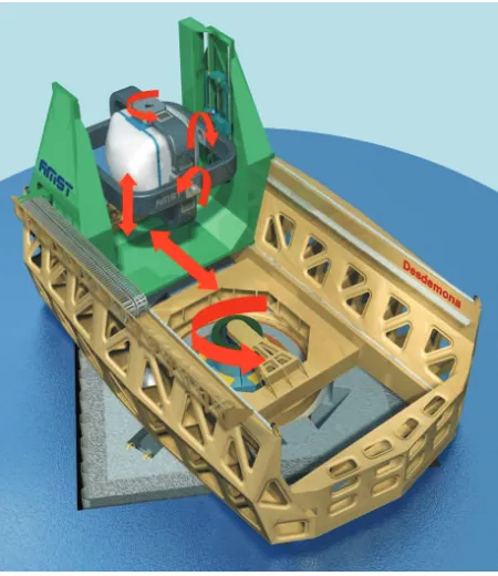
Human beings sense movements of their bodies. The interpretation of the sensed movements is a complex process and a broad research topic. For new research topics Desdemona is developed, it is a new kind of motion platform. With Desdemona it is possible to do research on the human perception model and to use the gained knowledge for applied research and applications. Some examples are the training for flying a plane, driving a car and steering a ship.

Figure 1.1: Desdemona at TNO

(14)

2 1. INTRODUCTION

1.1

Desdemona in comparison with other disorientation simulators

The1 most common motion platform is the Stewart six-pod platform, which allows all six degrees of freedom. Despite the fact that accelerations can be induced only for a short time, for many applications such as training for transport aircraft this platform is sufficient. However, for fighter aircraft with pulling high sustained G-loads, this platform is not sufficient for realistic mission rehearsal. Present developments show that for flight simulation with higher G-loads, centrifuges are built with roll and pitch options of the gondola. Problem with these simulators is that they are able to simulate the G-load, but that the corresponding angular accelerations during the onset, introduce conflicting motion information to the pilot’s equilibrium system. This may lead to unwanted side effects such as disorientation and motion sickness. Desdemona is a research simulator, which combines the possibilities of common Stewart platform with the possibility of the sustained G-load, however, without the co-varying rotational accelerations.

Figure 1.2: Desdemona movements

The Desdemona concept was developed by TNO Human Factors in co-operation with AMST Systemtechnik [2]. Figure 1.2 shows the concept. It consists of a fully gimbaled cockpit, which allows for unlimited rotation in all directions. The pilot with his head in the center of rotation, controls the (flight) instruments and has a view outside via up-to-date visuals. For simulation purposes different models and databases are available. The cockpit can move along an 8 meter horizontal track. The cockpit can also move vertically over 2 meter. Finally, the horizontal track is rotated around a vertical axis, which means that centrifuging is also possible. The working principle of a normal centrifuge is a variation on the angular velocity with constant eccentricity resulting in a varying G-load. However, keeping the angular velocity constant and varying the amount of eccentricity is another way of varying the G-load. Desdemona applies both with a maximal G-load of 3g. The main characteristic of the concept, i.e. the variation of the G-load by varying the eccentricity, has consequences for simulation. It means that the onset of a sustained G-load is not necessarily accompanied with a strong angular acceleration, as is the case in the conventional cen-trifuge. It is possible to start the rotator subliminal up to the desired speed with the cockpit in the center position, and subsequently move the cockpit away from the axis without varying the angular velocity. It is obvious that one should take into account the linear Coriolis accelerations during the movement of the cockpit on the track. This

(15)

DESCRIPTION OF THE PROBLEM 3

example also shows the difficulty of controlling Desdemona. It is possible to simulate a transversal acceleration by moving the cockpit on the horizontal track while possibly rotating the horizontal track. The choice depends on the magnitude and the duration of the desired acceleration.

1.2

Description of the problem

The control problem of the Desdemona is significantly different from that of the Steward platform, because the directions of movement of the Steward platform are in general the same as the model movements. Desdemona on the other hand can also use rotation to simulate a linear acceleration.

To find the optimal acceleration and rotation path, an optimal controller is needed. The optimal path is defined as the path that is as close as possible to the desired path.The optimal controller decides which movements of Des-demona give the best simulation of the desired path with taking constraints such as maximum power in account.

In this report an optimal controller is designed for the cases in which the acceleration trajectory is known and unknown beforehand.

1.3

Outline

(16)

(17)

Chapter 2

Objectives

Desdemona combines the degrees of freedom (d.o.fs) of a centrifuge simulator, used for sustained G-load simula-tion, with additional d.o.f.’s to give it the full 6 d.o.f. motion cueing possibilities of a standard hexapod simulator. In centrifuge mode, Desdemona rotates around its central yaw axis while in hexapod mode this axis, in combination with the main arm, is used to simulate linear accelerations. In both modes, attitude is simulated with the gimbaled system. The combination of a centrifuge and hexapod simulation mode provides huge advantages in simulations of highly agile maneuvers with sustained G-load (e.g.: F16 combat simulation, unusual attitude recoveries, etc.). The main objective of this report is to design an optimal motion cueing and control algorithm that takes full advantage of the available d.o.f’s of Desdemona.

Goal

The simulation of high frequency, agile motion in hexapod mode in combination with, or followed by, sustained G-loads in centrifuge mode requires advanced motion cueing and control algorithms. Although algorithms for the centrifuge and hexapod mode are developed by AMST separately, an algorithm that combines the two has not yet been developed. The goal of this work is to develop an optimal control algorithm that combines the centrifuge and hexapod capabilities of Desdemona during the simulation of highly agile maneuvers (high frequency accelerations) in combination with, or followed by, sustained G-loads (low frequency accelerations). In this scope, optimal is defined as:

• minimization of the perception of differences in the simulator

• minimization of false cues,

• within the limits of Desdemona (structural limits and drive limits).

Although pre-defined maneuvers will be used first, the ultimate, long-term goal is an optimal control algorithm that can be implemented in pilot-in-the-loop simulations (which will result in maneuvers that are hard to predict beforehand).

Methods

In order to reach the stated goal, the following sub-goals are defined:

• Study of literature on: modeling and simulation of robotic dynamics, optimal control concepts, Desdemona specifications, motion cueing in conventional flight simulation,

• Developing a dynamic simulation model of Desdemona,

(18)

6 2. OBJECTIVES

• defining an optimization cost function (incorporating perception of difference, false cues, drive performance parameters, etc.)

• developing & implementing of optimal control algorithms in the dynamic simulation model

• evaluating the optimal control algorithm, especially the ’optimal’ motion characteristics during the transition from hexapod motion types to centrifuge motion types (and vice versa).

(19)

Chapter 3

Problem definition for an optimal

controller

The main goal of the optimal controller is to find optimal movements for the jointsq(t)of Desdemona within the physical constraints such as motor power, dimensions etc.

To define the optimal control problem, the path and the error will be defined first and then the physical con-straints. At the end of this chapter a simplified model of Desdemona will be outlined.

3.1

Defining the path to be followed

Desdemona is a simulator, in which one feels the acceleration from the simulated model. The model gives output information on the rotation speedω(t)and the translation accelerationp¨(t)and gravityG(t). The calculated path from the model is the desired path for Desdemona and is indicated with:

Sd(t) =

µ

ωd(t)

¨

pd(t) +G(t)

¶

(3.1)

The mechanical part of Desdemona has to follow that path. The movement of Desdemona can be written in the same way as the movement of the model, but now as function of the joints and it derivativesq(t),q˙(t),q¨(t).

S(t) = µ

ω(q(t),q˙(t)) ¨

p(q(t),q˙(t),q¨(t)) +G(q(t)) ¶

(3.2)

Where omega can be extracted from the twist (see also A.6): T_headhead,earth = µ

ω v

¶

andp¨can be calculated

with equation A.18. The gravity vectorG(q(t))can be calculated with the help of the rotation matrix (see A.19).

The goal of Desdemona is to follow the path of the model. The error that Desdemona makes can be written as: ∆S(q(t),q˙(t),q¨(t), t) =Sd(t)−S(q(t),q˙(t),q¨(t)). The error that the pilot will observe is not∆S(q(t),q˙(t),q¨(t), t)

because the vestibular nerve system in combination with the visual input does not give an exact impression of ∆S(q(t),q˙(t),q¨(t), t). It is important to keep this in mind designing the optimum controller. This fact will be discussed later (chapter 6 ). But at this point it will be assumed that the pilot is observing∆S(q(t),q˙(t),q¨(t), t)as fault in the path.

3.2

Physical bounds of Desdemona

(20)

8 3. PROBLEM DEFINITION FOR AN OPTIMAL CONTROLLER

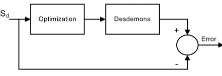
Optimization Desdemona

+

-Error

Sd

Figure 3.1: Optimal control problem

limited because they are the only two translation joints. The others are unbounded joint rotation movements.

−q2max≤q2(t)≤q2max

−q3max≤q3(t)≤q3max (3.3)

Other bounds on the velocities and accelerations prevent large mechanical stress and vibrations to occur in the system.

−q˙max≤q˙(t)≤q˙max

−q¨max≤q¨(t)≤q¨max

(3.4)

Desdemona is actuated by a number of motors and every motor has limited power and torque.

−Pi,max≤τi(t) ˙qi(t)≤Pi,max

−τmax≤τ(t)≤τmax

(3.5)

The power and torque relations are calculated in section A.4

3.3

Time horizon

Time horizon (Th) is defined as the amount of time in the future for which the desired path,Sd(t), is known.

The time horizons depend on the purpose the Desdemona is used. They can be grouped in two categories: man in the loop and no man in the loop (for example a roller coaster). If Desdemona works with man in the loop, the time horizon will be short although it is possible to predict a few seconds. This depends of course on the model which Desdemona is simulating. For example the path of a car which is driving on a road with no side lanes is easier to predict then a car on a road with side lanes. If there is no man in the loop then the time horizon runs till the end of the simulation, because the path is predefined.

3.4

Mathematical formulation of the optimization problem

Figure 3.1 shows the optimization problem. The problem can be calculated off-line for cases where there is no man in the loop. In case there is a man in the loop simulation, then the state at the end of the time horizon (final state) of Desdemona is important, since future simulation errors need to be avoided1_{. Because the path}_S

dcan not

be calculated in advance, the optimization should be done online.

The definition of the problem is divided an on-line and off-line optimization.

1_{With man in the loop the simulation time is longer than the time horizon and the path of Desdemona is optimized with several optimizations}

(21)

EXAMPLE OF THE OPTIMIZATION 9

The off-line optimization problem can be written as:

min

¨

q J =

Z te

t0

∆S(q(t),q˙(t),q¨(t), t)TQ∆S(q(t),q˙(t),q¨(t), t) dt (3.6)

subject to the Dynamical system:q¨(t) =f(q(t),q˙(t), τ(q(t),q˙(t),q¨(t)))(see section A.4), and the constraints:

|q2(t)| − q2max ≤0

|q3(t)| − q3max ≤0

|q˙(t)| − q˙max ≤0

|q¨(t)| − q¨max ≤0

|τ(t)| − τmax ≤0

¯

¯τi(t) ˙qi(t)T

¯

¯₋ Pi,max ≤0 (3.7)

whereQis a semi-positive definite weighing matrix. The elements of the matrix give to some extent the impor-tance of the optimization per direction of the path.q¨andτare calculated in A.27 and A.26

The on-line (real time) optimization problem can be written as:

min

¨

q J =K(q(te),q˙(te), te) +

Z te

t0

∆S(q(s),q˙(s),q¨(s), s)T_Q_∆_S₍_q₍_s₎_,_q_˙₍_s₎_,_q_¨₍_s₎_{, s}_{) d}_s _(3.8)

And is subjected to the same constants as in the off-line optimization. WhereK(q,q, t˙ e)gives the inverse of

the quality of the state of Desdemona atte. Quality of the state is defined as the possible accelerations Desdemona

can simulate at that point. If Desdemona is in a singular point thenKwill be large and if Desdemona can simulate all accelerations thenKwill be small.

3.5

Example of the optimization

3.5.1

Introduction

The problem of finding the right path for Desdemona can be made a bit easier by reducing it to a problem with two degrees of freedom. The problem itself will be the same ”find the optimal path”.

In this example only jointsq1andq2are considered. The other joints are fixed and for the fixed parts the inertia

is zero. The acceleration that the pilot should feel is taken as a cosine in theydirection of the cockpit. At this point the other accelerations (false cues) are not include in the optimization. The pathSdcan be defined by:

¨

y = cos(wt) (3.9)

Sd(t) =

        0 0 0 0 ¨ y 0         (3.10)

For the error only the acceleration in theeydirection is taken into account. Thus

Q=        

0 0 0 0 0 0

0 0 0 0 1 0

0 0 0 0 0 0

(22)

10 3. PROBLEM DEFINITION FOR AN OPTIMAL CONTROLLER

The constraints which are mentioned in paragraph 3.2 are valid.

The optimal controller should calculate the movements of the joints. The expectation is that if the frequency ofy¨is high enough, the linear sled will make sine movements and the rotation of the central yaw will remain zero. But for low frequencies the linear sled will not have enough space to move. It will reach the end of the vertical axis. Desdemona will use the central yaw to generate an acceleration in theydirection of the cockpit by centrifugal acceleration.

3.5.2

Mathematical formulation

The problem can be formulated as:

min

¨

q J =

Z te

t0

∆S(q(t),q˙(t),q¨(t), t)T_Q_∆_S₍_q₍_t₎_,_q_˙₍_t₎_,_q_¨₍_t₎_{, t}₎_dt _(3.11)

|q2(t)| − q2max ≤0

|q˙(t)| − q˙max ≤0

|q¨(t)| − q¨max ≤0

|τ(t)| − τmax ≤0

¯

¯τ(t) ˙q(t)T¯¯− Pmax ≤0

TheSand theτvector are calculated in appendix B

3.5.3

Outline of analytical solution

One of the basic methods to solve optimal problems is the Minimum Principle of Pontryagin [18]. To solve the optimal problem with the minimum principle of Pontryagin, the dynamic equation has to be rewritten as a first order differential equation and the constraints are rewritten as extra cost. The solution of the problem can then be rewritten as8ODE’s (ordinary differential equations) where 4 ODE’s have an initial value and 4 a final value. This is done in Appendix B.1.

The ODE’s can not be solved analytically with symbolic computer programs like Maple. It is possible to solve the equations numerically with the Matlab function ode45 which is based on an explicit Runge-Kutta [7]. The difficulty is that the method can only handle initial values. So the initial values have to be chosen in such a way thatp(the co-state, see section B.1) is zero atte. For somex0and some trivial weight functions of the cost function

(23)

Chapter 4

Numerical optimization

4.1

Introduction to numerical optimization

In this section the analytical optimization problem will be redefined as a numerical optimization problem. This numerical problem will be compared to other standard optimization problems to determine the right numerical optimization method. After that, the optimization method and their limitations will be discussed. At the end of this chapter the example from section 3.5.3 is solved using numerical optimization.

4.2

Redefining the analytical optimization to a numerical problem

The off-line optimization problem is given in equation 3.6. For the numerical case the cost function has to be written in a discrete form because integrating and differentiating are done in continues time and discrete time differently.

The integral of the joint vectorsq(k)is calculated with the discrete method Runge-kutta [7], whereq¨(k)is taken as input.

Thereafter the cost function and the constraints are be calculated. The integral in the cost function can be replaced with a sum operator, since the integral only integrates discrete values. This is elaborated in section D.2.

The input for the discrete cost function isq¨∈RM×N_{, where}_M_{is the number of d.o.f of}_{q, and N the number}

of time steps. All the time steps have to be optimized, therefore the number of parameters which have to be opti-mized isM×N.

The discrete optimization problem can now be written as:

min

¨

q J = te X

k=t0

∆S(q(k),q˙(k),q¨(k), t(k))TQ∆S(q(k),q˙(k),q¨(k), k) (4.1)

subject to

|q2(k)| − q2max ≤0

|q3(k)| − q3max ≤0

|q˙(k)| − q˙max ≤0

|q¨(k)| − q¨max ≤0

|τ(q(k),q˙(k),q¨(k))| − τmax ≤0

¯

¯τi(q(k),q˙(k),q¨(k)) ˙qi(k)T

¯

(24)

12 4. NUMERICAL OPTIMIZATION

Another way of writingJ is

J =

te X

k=t0

kf(t(k),q¨(k)k2 (4.3)

with

f(t(k),q¨(k)) =pQ∆S(q(k),q˙(k),q¨(k), k) (4.4)

and√Qsuch that(√Q)T√_Q₌_Q

4.3

Classifying the numerical optimization problem

The optimization problem can be grouped in two differed classes [17]. The first group is where the cost function depends on integer values. Examples where the cost function depends on an integer are routing in batch processes or path-length problems. The second group, is where the cost function depends on parameters with a real value, can be separated in the following subgroups.

Linear programming problem The cost function is linear or affine1

Quadratic programming problem The cost function is quadratic and the constraints are linear or affine. Nonlinear optimization problem The cost function is nonlinear, non-convex.

Convex optimization The cost function is a convex function. (A convex function has one local optimum (the

global minimum), see section C.1.3)

The numerical Desdemona optimization problem can be placed in the group nonlinear optimization problems. The numerical cost function defined in 4.1 is nonlinear and not quadratic because∆S is not linear and the cost function is not a quadratic function of the inputs. Another reason is that the cost function is non-convex and we expect local minima. A nonlinear optimization problems can be grouped in several classes. From equation 4.3 it is obvious that the Desdemona problem has the form which is called a least-squares (data-fitting) problem. The least-squares (data-fitting) problem has the from of:

min

x J(x) =f1(x) +f2(x) +. . .+fn(x)

4.4

Methods for solving nonlinear least-squares optimization problems

Most of the numerical optimization techniques work in combination with the Newton method (see appendix C.2). The Newton method in combination with the line search algorithm is selected for nonlinear least-squares optimiza-tion problems because it is used in [17] and [8], in [9] this method is also menoptimiza-tioned as opoptimiza-tion. In [4] this method is described for solving a Model Predictive Control (MPC) problem. A MPC problem is a online optimization problem. A global overview of the complete optimization method can be found in section D.1.1.

4.4.1

Methods with direction determination and line search

Each iteration step of these methods consists of a direction determination followed by a line search, i.e., an opti-mization along this determined direction. The basic idea is to choose a search directiondk at an initial pointxk,

and then to minimize the objective function J(x) along a line

xk+1=xk+dks s∈R

Wherexkanddsare vector andsis a scalar.

Now a one dimensional minimization problem can be obtained.

min

(25)

LIMITATIONS TO THE NUMERICAL OPTIMIZATION 13

The starting point for the next iteration is then given by

x(k+ 1) =x(k) +d(k)sopt(k)

where

sopt(k) =min

s J(x(k) +d(k)s)

The search direction can be calculated with the Newton methodd(k) =−H−1₍_x₍_k₎₎

∇T_J₍_x₍_k₎₎_{, or any other}

quasi-Newton method.

For the determination of the step size ofsare several methods available [17].

4.5

Limitations to the numerical optimization

The goal of every optimization is to find fast the global minimum of the optimization problem. This is a difficult problem because as stated before our optimization problem is a nonlinear and non-convex problem. This is also mentioned in [4] for solving a nonlinear MPC problem (which is comparable to our problem): ”The solution of this problem requires the consideration (and at least partial solution) of a non-convex, nonlinear problem (NLP) which gives rise to a lot of computational difficulties related to the expense and reliability of solving the NLP online”. Reference [13] shows that the minimum number of computations required to compute the global minimum of a general differentiable function innvariables, within an accuracy ofε, grows like,

µ 1 ε

¶n

(4.5)

roughly speaking, the complexity of a search over ann-dimensionalε-grid. If the function is convex, then the function becomes n log µ₁ ε ¶ (4.6)

Taking e.g. εequal to10−3

andn = 10, then we have the following complexity measures: for the non-convex function1030_{and for convex function equal to 30. This result shows that a non-convex problem is hard to solve.}

In a nonlinear and non-convex problem the used Newton method always finds local minima instead of global minima; this is unavoidable [17][9][3]. The only method to avoid this is to start optimizing with different initial values so that several local minima will be found, and hopefully (certainty is never present) the lowest is the global minimum.

The duration of the optimization is something which should stay small. This is specially imported for real time applications (like model predictive control). The main time consuming operation is the calculation of derivative of the cost function which has to be calculated in the Newton method. The calculations can be done in two ways. The best (fastest) method is to find an expression for the derivative, but this is not always possible, in which the deriv-ative has to be determined by numerically. It can be done by varying the input of the cost function and to calculate the output. This is a time consuming operation but the only way to find the derivative of our optimization problem2.

4.6

Converting a constrained to an unconstrained optimal problem

Nonlinear inequality constraints usually make the optimization problem more difficult. One common way to tackle the nonlinear inequality problem is to incorporate the constraints function in the objective function, using a barrier function.

2_{In the case of the dynamic flight simulator it is possible to calculate the derivative symbolical because of some trivial simplifications (see}

(26)

14 4. NUMERICAL OPTIMIZATION

If the optimization function has the constraintg(x)≤0then the basic idea of the barrier function is to introduce a feasibility functionJf easof the form

Jf eas(x) =

½

0 g(x)≪0 ∞ g(x)→0

and add this function to the original cost function

min

x [J(x) +Jf eas(x)]

In this way the cost function will increase significantly if the inequality constraints is not met, an example is:

Jf eas = −

1 βg(x)

withβ >1

4.7

Example of numerical optimization

The example which was drawn up analytically (see section 3.5.3) is now solved numerically. The pathSd(eq. 3.9)

will be redefined, namelyy¨= 5 cos(2t)

The constraints will be included using a feasibility function. It is taken the same as in the analytical optimization (eq. B.13).

The used parameters are: M1 = 1ie1

z = 1M2 = 2ie

2

z = 2(the other elements of Desdemona are assumed weightless)a = 0.1b = 1e−3 _c _{= 1}_e−5 _{(These parameters are taken as example, they are not realistic).} _The

step-size is taken0.1sec and the total time is 5 sec.

The initialsq(t0),q˙(t0))are taken random just asq¨(t0),q¨(t1), . . . ,q¨(te). Now the optimization can be done,

using 40 iterations in combination with the line search method.

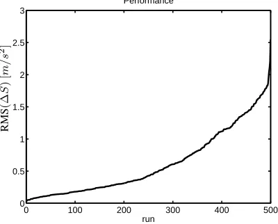
This optimization has been done 500 times (runs), every run with different initial values. This is done because the line search method finds a local optimum and this way it was tried to find the global minimum. These runs are sorted on performance (see figure 4.1), where the performance is the cost function without feasibility function . It can be seen that the initial values have an influence on the final results of the optimization.

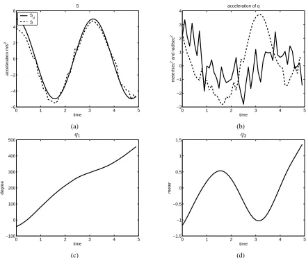
In figure 4.2 the results are given for run 300, so there are thus 299 runs with a better performance. The movement Desdemona is making is rotating and making small sinus movements around the origin with the vertical sledge. It can be seen that the accelerationsS are almost the same asSd. The values of joint vectorq2 are bounded. The

runs with a better performance have a similar behavior, the∆Sbecomes smaller andq2remains small. The main

(27)

EXAMPLE OF NUMERICAL OPTIMIZATION 15

0 100 200 300 400 500

0 0.5 1 1.5 2 2.5 3

run Performance

R

M

S

(∆

S

)

[

m

/

s

2]

(28)

16 4. NUMERICAL OPTIMIZATION

0 1 2 3 4 5

−6 −4 −2 0 2 4 6 S time acceleration m/s 2 S_d S

0 1 2 3 4 5

−3 −2 −1 0 1 2 3 4

acceleration of q

time

meter/sec

2 and rad/sec

2

(a) (b)

0 1 2 3 4 5

−100 0 100 200 300 400 500 time degree q1

0 1 2 3 4 5

−1.5 −1 −0.5 0 0.5 1 1.5 time meter q2 (c) (d)

Figure 4.2: In (a) the S (doted line) andSd (Solid line) are plotted. In (b) the vector q¨1 (solid line) andq¨2

the (doted line) are plotted. In (c) and (d) the vectorq1and respectively q2are plotted. The initial velocity is

˙

(29)

Chapter 5

Practical extensions of the numerical

optimization

In the previous chapter the optimization problem is solved for the most basic case. In this chapter the optimization problem is redefined to make it a more practical applicable optimization problem. Therefore the feasibility function is changed and the initial values of Desdemona (q(t0),q˙(t0)) are included as optimization parameter. The sample

times and stop criteria are chosen more carefully. At the end of this chapter some more realistic paths are defined and Desdemona is optimized with real parameters for the two and three d.o.f. cases.

In this chapter the following terminology is used: with run, a complete optimization. A complete optimization consists of a number of iterations. The performance of a run is given as the root mean Square (RMS) of∆S.

RM S(∆S) =

r Pn

i=1∆Si2

n (5.1)

These RMS sorted with the best run first is plotted in the next sections for a number of runs to compare several different optimization configurations.

5.1

Barrier functions

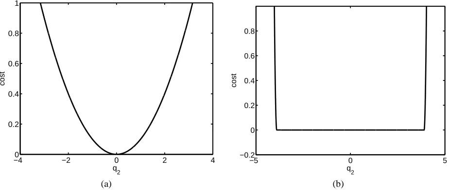
The barrier function (see section 4.6) is taken quadratic in the example (section 3.5 or 4.7). This is not a realistic barrier function because it results in costs when there is no reason for. This results in unwanted restriction of the joins and motor. This can be seen forq2in figure 5.1.a. ifq2= 2then it is not near the end of the track but there is

already a cost.

A good cost function is a cost function where the cost is low and constant if the constraints are not violated, if the constraints are (almost) violated then the cost function should increase significantly. The function should be continuous which is important when taking the derivative in the Newton method.

An example of a good barrier function is given in eq. 5.2 and can be seen in figure 5.1.b.

Jf eas(q2) =

½

((q2)2−3.72)2 |q2|>3.7

0 |q2| ≤3.7

(5.2)

To evaluate the cost function the experiment from section 4.7 is repeated, but now with the barrier function which is given in equation 5.2. The results are given in figure 5.2. The number of runs is chosen in such away the calculation time is reasonable and the results can be justified statistically and the number of iterations is taken big enough so that the results are satisfying. Further in this chapter there is discussed how to determine the right number.

(30)

18 5. PRACTICAL EXTENSIONS OF THE NUMERICAL OPTIMIZATION

−40 −2 0 2 4

0.2 0.4 0.6 0.8 1 q 2 cost

−5 0 5

−0.2 0 0.2 0.4 0.6 0.8 q₂ cost (a) (b)

Figure 5.1: Two differen types of barrier functions. (a) is a quadratic function and (b) is a combination of a quadratic function and an ’if’ statement.

0 100 200 300 400 500

0 0.5 1 1.5 2 run Performance (q 2) 2 if R M S (∆ S ) [ m / s 2]

Figure 5.2: Two experiments with different barrier functions. One run consists of an optimization with 40 itera-tions. The result (y-axis) of one run is the root mean square (RMS) of (∆S). In total 500 runs have been done which are sorted with the lowest cost first. The solid line is the result of the optimization with a quadratic feasibility function, this experiment is the same as in figure 4.1. The other line gives the result for an optimization with a feasibility function which is given in equation 5.2.

5.2

Optimizing initial position and speed of Desdemona

Every profile has an optimal for the initial position and speed. This can be seen in the example (figure 4.2) where the initial position and speed aren’t optimal which results in a relatively large difference(∆S)in the beginning of the path.

The initial position and speed can be optimized by including it in the optimization problem. Therefore the numerical optimization problem from section 4.2 is redefined. The original the cost functionJ only depends on

¨

q(·). The new cost function includesq(t0),q˙(t0), the new optimization problem is thus:J(q(t0),q˙(t0),q¨(·)).

(31)

OPTIMIZING WITH DIFFERENT STEP SIZE 19

0 100 200 300 400 500

0 0.5 1 1.5 2 2.5 3 3.5 4 run sqrt(( ∆ S)

2) [m/s

2]

original 40 itr 50 itr

Figure 5.3: Three experiments are plotted, the original problem and the optimization which include(q(t0),q˙(t0)).

The optimization is done with 40 iterations (40 itr) and with50iterations (50 itr). The results (y-axis) of one run is the root mean square (RMS) of (∆S).

The results can be found in figure 5.3. It can be seen that the solutions which optimize the initialq(0),q˙(0)give better results than the original solution. If the cost is larger then 1.5m/s2_{then the new optimization problem need}

50 iterations for getting the same performance. It can be understood intuitively that the new optimization prob-lem needs more iterations for some cases, because the larger the number of variables will make the optimization problem harder. This is also shown in the next section.

5.3

Optimizing with different step size

The numerical optimization problem works with a sampled version ofSd(t)andq(t). The numerical integration

method also works with a certain sample frequency for the continuous time ODE. These three sample frequencies can be chosen independently of each other. This is because the sample frequency of the iteration method (f sitr)

should be taken carefully to ensure numerical stability. The sample frequency forSd(t)isf sSdand forq(t)isf sq. They should be at least twice as big as bandwidth of respectivelySd(t)andq(t)because of the so called Nyquist

criteria [5]. Another reason for choosing the step size ofq(k)carefully, is that the larger the step size (the lower f sq) the smaller the number of parameters which have to be optimized. This results in easier problems.

The optimization problem is rewritten so that it is possible to optimize the problem with three different sample times. For the conversion between two sample times some values have to be re-sampled in a way such that there is no information lost. Therefore the new samples should be accurately interpolated. The conversion to a smaller step size is done by adding samples with value0and applying an anti-aliasing (lowpass) filter to the re-sampled value (with compensation for the filter’s delay). For the conversion to a larger step size first a anti-aliasing filter is applied and after that some sample are deleted. This technique is described in [5]. The new cost function is given schematically in section D.2.

hu[s] computing time [s]

0.1 101.6

0.2 52.1

0.5 22.3

1.0 12.5

Table 5.1: The average computing time (simulated with a AMD Athlon 1800) that is needed for one optimization run is given categorized per sample time.

(32)

20 5. PRACTICAL EXTENSIONS OF THE NUMERICAL OPTIMIZATION

0 100 200 300 400

0 0.5 1 1.5 2 run Performance h q=0.1s h q=0.2s h q=0.5s h q=1s R M S (∆ S ) [ m / s 2]

Figure 5.4: Four experiments optimizing with different step sizes, in the legends the sample time is given. The results (y-axis) of one run is the root mean square (RMS) of (∆S).

is the same as the original experiment (section 4.7) but now with different step size and number of iterations (see for the definition of iteration section 4.4.1). The step size ofSd(k)is taken ashSd = 0.1sand the step size of the numerical integration method is changed tohitr = 0.05s. The step-size of the numerical integration is not changed

during the experiment. The step size ofq¨(k)is changed during the experiment betweenhq¨= 1sandhq¨= 0.1s

(original optimization problem). The optimization is done with 20 iterations.

In figure 5.4 and table 5.1 the results are given. The original optimization problem with sample timehSd= 0.1s has the worst performance. This can be seen from the high cost and computing time. This is due to the number of variables which have to be optimized. The fewer variables (the larger the step size) that have to be optimized, the easier (faster) it is to optimize. The is that the sample frequency ofqcan not be taken to low because then it is not possible to include the high frequency accelerations. This will be shown in the next experiment.

From the previous paragraph it is clear that for a last optimization the lowest possible sample frequency ofq(t) should be determined prior to the optimization. When the path of Desdemona is a linear function of the states of the jointsS(q(t),q˙(t),q¨(t), t), then the sample frequencies ofSandqcan be taken the same. But because Desdemona is nonlinear this is not the case1_{. The only relation is that the higher the frequencies in}_S

d(t)the higher the sample

frequency has to be forq(t).

In the following experiment it will be shown that there is a relationship between the step-size ofq(k)and the frequency inSd(k). The following step sizes are used:hSd= 0.1s,hitr = 0.05sandhq¨= 1s. The frequency of the accelerations inSd(k)is changed from 2 to 5rad/s, the results are shown in figure 5.5. If the frequency ofSd

is above 3 rad/s the cost is increasing enormously. This is due to a too low sample frequency forq(k). So it can be concluded that the frequency ofSd(k)has an influence on the neededf sq.

5.4

Different stopping criterions

In previous experiments the number of iterations in a optimization run is fixed. This is not a logic stop criteria because if the optimization method finds the (local) optimum in fewer steps, the additional steps do not doesn’t benefit the performance. Therefore the optimization should be stopped if the optimum is reached. If the optimiza-tion has reached its optimum then the change in the cost funcoptimiza-tion will remain small in the next iteraoptimiza-tion steps. So, a good extension of the stop criteria is adding a minimum for the change of the cost function. If the cost function is changing less then the minimum, the optimization will be stopped.

This extended stop criterium has been tested in the following experiment. The minimum change for the stop criteria is taken0.1. The results are given in figure 5.6. The performance is almost the same hence the extra stop

1_{It is possible for some nonlinear filter cases to calculate the output frequency for a given input frequency. But for Desdemona this is not}

(33)

EVALUATING DIFFERENT PROFILES 21

0 5 10 15 20

0 0.5 1 1.5 2 2.5 3 3.5 4 Performance run ω=2 ω=3 ω=4 ω=5 R M S (∆ S ) [ m / s 2]

Figure 5.5: Four times the experiment of section 4.7 is done with four differentSd(k). TheSd(k)in equation 3.9

is defined asy¨= 5 cos(ωk)withωchanging between 2 and 5 rad/s. The results (y-axis) of one run is the root mean square (RMS) of (∆S).

criterium is not influencing the results. But there is a30%saving of computing time, hence the extended stop criterium is useful.

0 100 200 300 400 500

0 0.2 0.4 0.6 0.8 1 1.2 1.4 1.6 1.8 2 Performance run original stop criteria R M S (∆ S ) [ m / s 2]

Figure 5.6: Different stopping criterions, the results of the original experiment (section 4.7) with 40 iterations and the same experiment with extra stop criterium. The extra stop criterium will stop the optimization if the changing of cost function(inclusive feasibility function) is below 0.1. The results (y-axis) of one run is the root mean square (RMS) of (∆S).

5.5

Evaluating different profiles

The final step in the two degrees optimization problem is to combine the new techniques described in this chapter. Another step is to use the real parameters (see section A.5) for dimensioning Desdemona and the motors. This optimization problem is tested with some realistic paths.

(34)

22 5. PRACTICAL EXTENSIONS OF THE NUMERICAL OPTIMIZATION

In this optimization problem all the constraints (see section 3.4) will be taken into account. For the feasibility function the barrier function in the form of equation 5.2 is chosen. The parameters which determine the bounds of the constraints can be found in section A.5.

5.5.1

Cosine path

To be able to compare the new realistic system with previous experiments the original cosine path will be used for the first experiment. The initial position is also optimized, and the stop criterium is taking the change of the cost function in account. The results for the best run is given in figure 5.7. The result is good because the constraints are met andSis very close toSd

5.5.2

Catapult start

This profile describes the start of an airplane from a aircraft carrier. It is a very strong acceleration in one (ey)

direction. The optimization also optimized the initial position as well. The results for the best run is given in figure 5.8. As can be seen there is a difference betweenSandSdalthough the flanks ofSare steep.

5.5.3

Triple pulse

The initial position is also optimized, and the stop criterium is taking the change of the cost function in account. The results for the best run (figure 5.9) are the same as the results of the catapult start, there is a difference between SandSdbut the flanks are steep.

5.5.4

Fast care

In this experiment the data from a real car is used. The accelerations are measured during 35 second while the car is doing the track from figure 5.10.

(35)

EVALUATING DIFFERENT PROFILES 23

plaatjes_two/COS_TWO_output_S.eps

(a)

plaatjes_two/COS_TWO_output_q1.eps plaatjes_two/COS_TWO_output_q2.eps

(b) (c)

plaatjes_two/COS_TWO_output_tau.eps plaatjes_two/COS_TWO_output_power.eps

(d) (e)

Figure 5.7: The best results for the cosines experiment. In (a) theS(doted line) andSd(Solid line) are plotted.

(b) and (c) are the positions of the jointsq1 andq2respectively are plotted. In (d) and (e) the normalized force

(36)

24 5. PRACTICAL EXTENSIONS OF THE NUMERICAL OPTIMIZATION

plaatjes_two/CAT_TWO_output_S.eps

(a)

plaatjes_two/CAT_TWO_output_q1.eps plaatjes_two/CAT_TWO_output_q2.eps

(b) (c)

plaatjes_two/CAT_TWO_output_tau.eps plaatjes_two/CAT_TWO_output_power.eps

(d) (e)

Figure 5.8: The best results for the catapult start. In (a) theS (doted line) andSd (Solid line) are plotted. (b)

and (c) are the positions of the joints are plotted. In (d) and (e) the normalized force and power respectively are plotted. It is normalized by dividing the force and power respectively by its maximum allowed value. If the normalized force or power is larger, then one, than one of the motors will be damaged. The initial velocity is

˙

(37)

EVALUATING DIFFERENT PROFILES 25

plaatjes_two/DUB_TWO_output_S.eps

(a)

plaatjes_two/DUB_TWO_output_q1.eps plaatjes_two/DUB_TWO_output_q2.eps

(b) (c)

plaatjes_two/DUB_TWO_output_tau.eps plaatjes_two/DUB_TWO_output_power.eps

(d) (e)

Figure 5.9: The best results for the double pulse experiment. In (a) theS(doted line) andSd(Solid line) are plotted.

(b) and (c) the positions of the joints are plotted. In (d) and (e) the normalized force and power respectively are plotted. It is normalized by dividing the force and power respectively by its maximum allowed value. If the normalized force or power is larger then one, than the motors will be damaged. The initial velocities are is

˙

(38)

26 5. PRACTICAL EXTENSIONS OF THE NUMERICAL OPTIMIZATION

plaatjes_alg/track.eps

(39)

EVALUATING DIFFERENT PROFILES 27

plaatjes_two/AUTO_TWO_output_S.eps

(a)

plaatjes_two/AUTO_TWO_output_q1.eps plaatjes_two/AUTO_TWO_output_q2.eps

(b) (c)

plaatjes_two/AUTO_TWO_output_tau.eps plaatjes_two/AUTO_TWO_output_power.eps

(d) (e)

Figure 5.11: The best results for the fast care experiment. In (a) theS(doted line) andSd(Solid line) are plotted.

(b) and (c) the positions of the joints are plotted. In (d) and (e) the normalized force and power respectively are plotted. It is normalized by dividing the the force and power respectively by its maximum allowed value. If the normalized force or power is larger then one, than the motors will be damaged. The initial velocities are is

˙

(40)

28 5. PRACTICAL EXTENSIONS OF THE NUMERICAL OPTIMIZATION

5.6

Desdemona with three degrees of freedom

A logical step to make the optimization problem more realistic is to increase the number of d.o.f. Thereforeq5the

yaw of the cabin is included. With this extra d.o.f. it is possible to place the cabin in every position in theex ey

plane of the fixed world and to simulate any desired acceleration profile (that is within bounds). In this section the same experiments are done as in section 5.5. All the experiments optimize also the initial position, and the stop criterium is taking the change of the cost function in account. In the pathSdthe linear translation inex ey

direction are defined, the rotation is not taken into account. The rotation is not taken into account because for example the catapult start path demands for almost 2 seconds an acceleration of20m/s2_{which result in a linear 40}

meter displacement or a combination of a small displacement and rotation. Desdemona isn’t 40 meter long, so we expect the optimal controller to force Desdemona to start rotating. Qis defined so that the rotation isn’t included in the optimization.

The results of the experiments are discuss in section 5.8.

5.6.1

Cosine path

To be able to compare the new realistic system with previous experiments the original cosines path will be used for the first experiment. The results for the best run is given in figure 5.12. The result is good because the constraints are met andSis very close toSd.

5.6.2

Catapult Start

This profile is from the start of an airplane from a aircraft carrier. It is very strong acceleration in one (ey) direction.

The optimization also optimized the initial position. The weight matrixQ(see section 3.4) is taken so that an error inexdirection result in a three times larger cost than ineydirection. The results for the best run is given in figure

5.13. It can be seen that the results aren’t so good as the two degree problem, this is to be expected because it is a much harder problem. The false cue (Sx) is smaller then the wanted acceleration (Sy) which is one of the basic

requirements to make the simulation realistic.

5.7

Improving the performance

In previous section Desdemona simulated with three d.o.f. The results can be increased by simplifying the dynamic model of Desdemona and by taking initial values not randomly but by selecting promising values. This is explained in this section.

Simplifying the dynamic model

The parameters of the dynamic are given in appendix A.5. The center of mass is not always in the origin of Desdemona coordinates. This makes the dynamic model more complex because it increases the number of joints that are influencing each other torques. By assuming the the center of the mass is always in the origin, some small errors are introduced in the optimization. The result is that the calculation time is shorter. The fact that some small errors are introduced can be eliminated by an extra optimization with the full dynamic model at the end. Thus this method is increasing the performance.

Smart Guess

All the experiments are until now done with random initial values (randomq(0),q˙(0),q¨(·)). But due to other research2 about Desdemona there are ideas of good performing inial values. Some experiments are done with these inial values. The idea is that a initial values that are chosen with prior knowledge give better results.

For example, if we expect anSd in theeydirection, where at the begin no accelerations and later some high

acceleration occur, then three groups of sensible initial parameters can be chosen, see table 5.2.

q2 q˙1 q˙2

0 _↑

-↑ 0 0

small _↑ _↓

Table 5.2: The three possible initial parameters. The_↑ means a large value. The acceleration will be low for a limited time and thereafter high. This can be found from equation B.5

5.7.1

Catapult start

The catapult start is repeated but now with a simplified dynamics and smartly guessed initials values.q(0),q˙(0):

[q1q2q5] = [0degree −0.01m0degree]

[ ˙q1q˙2q˙5] = [86degree/s −1.4m/s0degree/s]

The results are given in figure 5.16. The optimization with the simplified dynamics is done first and thereafter an optimization with the real dynamic is done to ensure the results are applicable to the Desdemona.

(46)

34 5. PRACTICAL EXTENSIONS OF THE NUMERICAL OPTIMIZATION

plaatjes_THREE/CAT_THREE_smart_Sx.eps plaatjes_THREE/CAT_THREE_smart_Sy.eps

(a) (b)

plaatjes_THREE/CAT_THREE_smart_q1.eps plaatjes_THREE/CAT_THREE_smart_q2.eps

(c) (d)

plaatjes_THREE/CAT_THREE_smart_q5.eps

(e)

Figure 5.16: The best results for the smart catapult experiment. In (a) and (b) the Sx andSy respectively are

plotted. In (c), (d) and (e) the positions of the jointsq1,q2andq5respectively are plotted. The constraints are not

(47)

DISCUSSION THREE D.O.F. RESULTS 35

5.8

Discussion three d.o.f. results

The results are good for the cosines experiment (figure 5.12). Thus the method is working. For the other exper-iments (figure 5.13, 5.14 and 5.15) the result are not as good. This is because the cost function is non-linear and non-convex, which result in a large number of local minima. In the two degree optimizations cases the problem is less nonlinear and therefore there are fewer local optimums.

For finding a low local minimum you need a huge number of trials. This number can be reduced by using promising initial values and by simplifying the dynamic model. But then you need a way to find these values. An example can can be found in section 5.7.

The cosines experiment has the best result, this is because the lower the existing frequencies inSd(t)are, the

easier to solve the optimization problem. One reason is you can resample the problem, and solve easier (see section 5.3). Or in other words, a change at a certain time of the joints of Desdemona will not only influence the error (∆S) at the same time interval but also in later intervals. This is particular the case ifSd(t)contains only lower

frequencies since there is more correlation between two sample next to each other.

Another difficulty is that the optimization has to deal with a huge number of input variables, for the fast car experiment (figure 5.15) 450 variables, which cause a huge complexity for the problem (see section 4.5).

Thus the results could be expected because of the known limitations and complexity (see section 4.5). Some options give better results by choosing better initial values, and to avoid high frequencies inSd(t)

If the optimization find a local minima, a method that possibly can be used to find other local minima in the neighborhood can be applied. The method redefines theSd(·)as

Sdnew(·) =λSd(·) + (1−λ)S(·)

withλ ∈< 0. . .1 >andS(t)is the path from the previous found optimum. Then with a new optimization run theSdnew(t)can be used to find other local minima. This method has been implemented with severalλand tested

(48)

(49)

Chapter 6

Including human perception model

6.1

Introduction

As stated before, the main goal of Desdemona is to let the person in Desdemona observe the same movements as in the simulated vehicle. Sometimes a human observes different movements than the human body it is making due to measurement faults. Therefore it is not always necessary that Desdemona makes the same movements as the simulated vehicle. By taking this into account it is possible to filter out irrelevant movements (movements a human doesn’t observe) and concentrate on the movements that a human does percept. To achieve this, a human perception model is included in the optimization problem, this is given in figure 6.1.

Desdemona Human

perseption +

-Error

Human perseption Optimization

Sd

Figure 6.1: A schematic model of the optimization problem with human perception model

6.2

Human perception

There are three main sensory systems involved in spatial orientation and disorientation: the visual system, the vestibular system (inner ear), the somatosensory system (”seat of the pants”)[1]. To a smaller degree, the auditory system is also involved. Of these, vision is by far the most important sensory system providing spatial orientation during flight. In the absence of vision, orientation must be derived solely from the vestibular or somatosensory systems, and these systems do not always provide accurate motion and position cues.

The primary role of the vestibular system is to enhance vision. It provides angular and linear acceleration information to stabilize the eyes when motion of the head and body would otherwise result in blurred vision. It’s secondary role, in the absence of vision, is to provide a sense of position and motion.

(50)

38 6. INCLUDING HUMAN PERCEPTION MODEL

example, if you sit in the train, you think it is leaving but instead it is nearby a train that is leaving

A fixed simulator involves virtual and auditory simulation and a moving simulator also involves the vestibular and somatosensory simulation. This work only deals with the moving part of Desdemona and in dialogue with TNO there has been decided to include the vestibular system in the optimization problem.

6.3

Vestibular system

Figure 6.2: The Vestibular system (from [12])

The vestibular system can be divided in the semi-circular canals and otoliths see 6.2. With these two perception models it is possible to measure rotation and linear acceleration. These models will be included in the cost function of the optimization and the new optimization will minimize the error in perception.

6.3.1

The semi-circular canals

The semicircular canals are part of the vestibular system. There are three semicircular canals located in the inner ear on each side of the head. Fluid within the canals moves relative to the canal walls when angular accelerations are applied to the head. This fluid movement bends sensory hair filaments in specialized portions of the canals, which send nerve impulses to the brain resulting in the perception of rotary motion. Each canal is oriented such that it responds differently from the others to angular accelerations in the pitch, roll and yaw spatial planes (see figure 6.3).

(51)

VESTIBULAR SYSTEM 39

The relative responses from all three canals are integrated by the brain to determine the actual plane in which the motion is occurring.

Dynamic model of the semi-circular canals

The model of the semi-circular canals are based on an overdamped-torsion-pendulum with transfer function

Hscc(ω) =

neural discharge rate angular acceleration =

K

(1 +τ1jω)(1 +τ2jω)

(6.1)

The technique to measure the neural discharge rate (impulses per second, ips) of the primary neurons in the vestibu-lar nerve, made the determination of the transfer function of the semi canals possible [6]. The transfer function becomes:

Hscc(ω) =

K(1 +τLjω)

(1 +τ1jω)(1 +τ2jω)

(6.2)

With the following parameters given in the table 6.1.

K 2ips/m/s2

τn 0.11s

τ1 5.9s

τ2 0.005s

Table 6.1: The parameters of the model (eq. 6.2) of the semi-circular canals. (ips stands for the Neural discharge rate (impulses per second)

Because in the used pathS the angular displacement is given as omega and not as acceleration the transfer functionHscchas to be differentiated. This is done with a lead filter [14] because a pure differentiator is difficult

to implement. The transfer function of the lead filter is jω

jω

α+1

whereαis chosen larger than the bandwidth of

Desdemona (see section A.5) so the lead compensation doesn’t have influence in the relevant frequency domain. The final transfer function can be found in eq. 6.3 and is plotted in figure 6.4.

Hscc(velocity)(ω) =

K(1 +τLjω)

(1 +τ1jω)(1 +τ2jω)

jω

α + 1

(6.3)

10−2 10−1 100 101 102 −90 0 90 Phase (deg) −30 −25 −20 −15 −10 −5 Magnitude (dB)

(52)

40 6. INCLUDING HUMAN PERCEPTION MODEL

6.3.2

The otoliths

The otolith organs are one of the sensory components of the vestibular system. They translate gravitational and inertial forces into spatial orientation information - specifically, information about angular position (tilt) and linear motion of the head. The otolith organs (see figure 6.5) contain top-heavy hair-like cells that bend in response to gravitational or linear acceleration forces. The bending of the sensory hairs relative to the membranes / structures to which they are attached are transformed into orientation signals to the brain. Inertial forces associated with the movement of the human body, combined with gravity, act upon the otolith organs.

Figure 6.5: The otholits (from [12])

Dynamic model of the otoliths

Considering their physical structure, each otolith can be modelled as an acceleration meter with over-damped mass-spring-dashpot characteristics [6]. The transfer function is given as:

Hoto(ω) =

neural discharge rate linear acceleration =

K

(1 +τ1jω)(1 +τ2jω)

(6.4)

It has been very difficult to identify the time constants. The main reason is the lack of adequate experimental installations to generate necessary linear acceleration stimuli. Based on different arguments, researchers concluded that the numerator of equation (6.4) should be extended with a first-order term [6] to:

Hoto(ω) =

K(1 +τnjω)

(1 +τ1jω)(1 +τ2jω)

(6.5)

with the following parameters given in table 6.2. The transfer function is plotted in figure 6.6. It can be seen that the otolith is most sensitive to movements between 0.1 and 10 hertz.

K 3.4ips/m/s2

τn 1s

τ1 0.5s

τ2 0.016s

Table 6.2: The parameters of the model (eq. 6.5) of the otoliths. (ips stand for the Neural discharge rate (impulses per second, ips)

6.4

Including model of the semi-circular canals and the otoliths

(53)

RESULTS 41

10-2 10-1 100 101 102 103

-90 0 90 Phase(deg) -20 -10 0 10 20 Magnitude(dB) Bode Diagram Frequency (Hz)

Figure 6.6: The bode plot of the otoliths transfer function eq. 6.5.

6.5

Results

6.5.1

Catapult Start

This experiment is an extension from the experiment which has been presented in section 5.6.2. The extension is that the effect of the otoliths are now included, the semi-circular canals are not included because in the original experiment the rotation is also not taken in to account. The result is given in figure 6.7 and 6.8. In figure 6.7 the output of the otoliths are given. It can be seen that a the otoliths are sensitive for an abrupt change in the accelera-tion (called jerk moaccelera-tion).

The results are better in comparison with the results from the same experiment without human perception model (see section 5.6.2). This is because the perception model is sensitive for acceleration changing which results in a steep acceleration pulse.

0 1 2 3 4 5

−20 −10 0 10 20 30 40 Sx(perc) time acceleration m/s 2 S dx(perc) Sx(perc)

0 1 2 3 4 5

−20 −10 0 10 20 30 40 Sy(perc) time acceleration m/s 2 S dy(perc) Sy(perc) (a) (b)

Figure 6.7: The best results for the three d.o.f. catapult start experiment. In (a) and (b) theSx,perc (perception,

(54)

42 6. INCLUDING HUMAN PERCEPTION MODEL

plaatjes_OOR/CAT_OOR_output_Sx.eps plaatjes_OOR/CAT_OOR_output_Sy.eps

(a) (b)

plaatjes_OOR/CAT_OOR_output_q1.eps plaatjes_OOR/CAT_OOR_output_q2.eps

plaatjes_OOR/CAT_OOR_output_q5.eps

(e)

Figure 6.8: The best results for the three d.o.f. catapult start experiment. In (a) and (b) respectivelySxandSyare

plotted. In (c),(d) and (e) the positions of the joints respectivelyq1,q2andq5are given. The constraints are not

(55)

An optimal controller for Desdemona for an optimal feeling

University of Twente

Summary

Nomenclature

Symbols

Abbreviations and used terms

Contents

1 Introduction 1

7 Predictive optimal control 43

Chapter 1

2 1. INTRODUCTION

Desdemona in comparison with other disorientation simulators

DESCRIPTION OF THE PROBLEM 3

Description of the problem

Outline

Methods

6 2. OBJECTIVES

Chapter 3

Defining the path to be followed

Physical bounds of Desdemona

8 3. PROBLEM DEFINITION FOR AN OPTIMAL CONTROLLER

Time horizon

EXAMPLE OF THE OPTIMIZATION 9

Example of the optimization

10 3. PROBLEM DEFINITION FOR AN OPTIMAL CONTROLLER

Mathematical formulation

Chapter 4

Redefining the analytical optimization to a numerical problem

12 4. NUMERICAL OPTIMIZATION

Classifying the numerical optimization problem

Quadratic programming problem The cost function is quadratic and the constraints are linear or affine. Nonlinear optimization problem The cost function is nonlinear, non-convex.

Methods for solving nonlinear least-squares optimization problems

LIMITATIONS TO THE NUMERICAL OPTIMIZATION 13

Limitations to the numerical optimization

Converting a constrained to an unconstrained optimal problem

14 4. NUMERICAL OPTIMIZATION

Example of numerical optimization

EXAMPLE OF NUMERICAL OPTIMIZATION 15

Chapter 5

Barrier functions

18 5. PRACTICAL EXTENSIONS OF THE NUMERICAL OPTIMIZATION

Optimizing initial position and speed of Desdemona

OPTIMIZING WITH DIFFERENT STEP SIZE 19

Optimizing with different step size

20 5. PRACTICAL EXTENSIONS OF THE NUMERICAL OPTIMIZATION

Different stopping criterions

EVALUATING DIFFERENT PROFILES 21

Evaluating different profiles

22 5. PRACTICAL EXTENSIONS OF THE NUMERICAL OPTIMIZATION

Cosine path

Triple pulse

EVALUATING DIFFERENT PROFILES 23

EVALUATING DIFFERENT PROFILES 25

26 5. PRACTICAL EXTENSIONS OF THE NUMERICAL OPTIMIZATION

28 5. PRACTICAL EXTENSIONS OF THE NUMERICAL OPTIMIZATION

Desdemona with three degrees of freedom

Cosine path

Double pulse

DESDEMONA WITH THREE DEGREES OF FREEDOM 29

30 5. PRACTICAL EXTENSIONS OF THE NUMERICAL OPTIMIZATION

DESDEMONA WITH THREE DEGREES OF FREEDOM 31

32 5. PRACTICAL EXTENSIONS OF THE NUMERICAL OPTIMIZATION

IMPROVING THE PERFORMANCE 33

Improving the performance

Simplifying the dynamic model

Catapult start

34 5. PRACTICAL EXTENSIONS OF THE NUMERICAL OPTIMIZATION

DISCUSSION THREE D.O.F. RESULTS 35

Discussion three d.o.f. results

Chapter 6

Human perception

38 6. INCLUDING HUMAN PERCEPTION MODEL

Vestibular system

VESTIBULAR SYSTEM 39

40 6. INCLUDING HUMAN PERCEPTION MODEL

The otoliths

Dynamic model of the otoliths

Including model of the semi-circular canals and the otoliths

RESULTS 41

Results