A discrete-time queueing model of the shared buffer ATM switch with bursty arrivals

A discrete-time queueing model of the shared buffer ATM switch

with bursty arrivals

1

S. Hong and B.G. Perros

Computer Science Department and

Center for Communication and Signal Processing North Carolina State University

Raleigh,

NC

27695-8206, U.S.A.

and

H. Yamashita/

Mechanical Engineering Dept. Sophia University Kioi-cho 7-1, Chiyoda-ku

Tokyo 102, Japan

Abstract

\Ve model the shared buffer ATM switch as a discrete-time queueing system. The arrival process to eachport oftheATM switch.isassumed to be bursty and it is modelled by an Interrupted Bernoulli Process. The discrete-time queueing system is analyzed approximately. It is first decomposed into subsystems, and then each subsystem is analyzed separately. The results from the subsystems are combined together through an iterative scheme. The analysis of each subsystem involves the contruction of the superposition of all the arrival processes to the switch. Comparisons against simulation data showed that the approximate results have a good accuracy.

1

Introduction

Many ATM switch architectures have been proposed so far. These architectures can be classified int~ the follo~gthree categories: space-division, medium sharing, and buffer sharing (see To-bag! [22]). In this paper, we are concerned with modelling the shared buffer switch architecture. In this type of switch architecture, there is a single memory which is shared by all input and output ports. All incoming and outgoing cells are kept in the same memory. The size of the memory is fixed so that it corresponds to a specific cell loss. An example of this type of switch architecture is the Prelude architecture (see Devault, Cochennec, and Serve! [5]). Also see Kuwahara et al (12],

and Lee et al

[13].

Analytic performance models of the shared buffer switch architecture have been proposed under the assumption of Bernoulli arrivals. These models are based on the analysis of a single

GeoiD

11

infinite capacity queue. The results obtained from this queue are used to analyze the whole switch which is represented by N identical GeoiD/1 queues. In particular, Brunee1 and Steyaert

[4]

obtained the N-fold convolution of the queue-length distribution of a Geo/D

/1

queue. Using this convolution, they derived the queue-length distribution ofN GeoiD

/1

queues. Eckberg and Hou [6] proposed a heuristic method which involved the following two steps. First, derive the mean and variance of the number of cells in N Geo/D/1 queues. Then, choose a well known distribution, characterized by its first two moments, which closely approximates the real queue-length distribution in a shared buffer switch. For further details see Petit and Desmet [18]. See also Boyer et al [3], and Petit et al [17].

In this paper, we model the shared buffer switch by a discrete-time queueing system which explicitly represents the input and output ports and the queueing of cellsin the shared buffer. The arrival process to each input port is assumed to be an Interrupted Bernoulli Process (ffiP). We analyze the queueing system approximately by decomposing it into subsystems. Each subsystem is analyzed separately. The results from the subsystems are combined together through the means of an iterative scheme.

The analysis of a subsystem is quite complex due to the large number of arrival processes. One way of analyzing a subsystem is to first obtain the superposition of all the arrival processes, and then analyze it assuming a single arrival process. This approach reduces the dimensionality of the problem. However, it requires the construction of the superposition process which is a fairly

complex problemin itself. This problemhasreceiveda lot ofattentionin theopen literature. One

approach for obtaining the superposition process focuses on approximating it by a renewal process, see Albin (1], Whitt [23], Sriram and Whitt [21], Iscoe, McDonald, and Qian [9], and also Perros and Onvural [16]. Heffes and Lucantoni [8] proposed a method for superposing approximately voice sources using a Markov ldodulated Poisson Process (MMPP). An alternative method for constructing an MMPP approximation to the superposition of identical bursty sources was proposed by Baiocchi et al [2]. Finally, Heffes

[7]

obtained an MMPP approximation to the superposition of different MMPP arrival processes using a set of simple expressions.

mul-tiplexer, see for instance, Nanos et a.l

[15],

Sengupta [20J, and Nagarajan, Kurose, and Towsley

[14J.

~or ftut~er reference, see Pujolle and Perros

[19].

We note that most of the methodologies reported

in ~he litera.ture for the analysis of an ATM multiplexer have been obtained assuming identical

~valprocesses. However, this assumption is unrealistic since in a real ATM network it ishighly unlikely that all patterns of arriving cells willbe identical.

The remaining of the paper is organized as follows. In the following section, we describe in detail the queueing model of the shared buffer switch, In section 3, we present the approximation algorithm, and in section 4, we validate the approximation algorithm by comparing it against simulationdata. Finally,the conclusions are givenin section 5.

2

Model Description

An ATM switch routes incoming cells from input ports to their destination output ports. The mechanism to route incoming cells to their requested output ports can be implementedin various ways.

In

the shared buffer switch architecture, all incoming cells are stored in a shared buffer and their memory addresses are stored inaddress queues. There is one address queue per output port. All memory addresses in an address queue point to cells in the shared buffer which are destined for the same output port. The address queue can be implemented in different ways. For instance, an address queue can be implemented as a linked list (see Kuwahara et a1 [12]) or it can be stored

in a FIFO buffer which is dedicated to a specific output port

(see

Lee et

a1

[13]). The shared memory has a finite capacity. Also,limitations can be imposed on the size of each address queue. A cell will be lost ifit arrives to find the shared buffer full It willalso be lost ifthe shared buffer is not full, but its address queue is full. The switch architecture is synchronized. Between two synchronization points any incoming cells that are in process of arriving at the input ports are written to the memory, and eachoutput port transmits a cell

(if

there is oneinits address queue).

An important factor that affects the performance of an ATM switch is the burstiness of the arrival process to each port. In this paper, each arrival process is assumed to be bursty and it is modelled by an Interf"Upted Bernoulli Proce•• (IBP). The burstiness of an arrival process is measured by the squared coefficient of variation of the interarrival time. An ffiP process mayfind itself either in the busy state orin the idle state. Arrivals occur in a Bernoulli fashion only when the process i. in the busy state. No arrivals occurifthe process is in the idle state. Let us assume that at the end of slot t the process isin the idle (orbU5Y) state. Then,in the next slot t

+

1it will

remainin the idle (or busy) state with probability

q

(or

p),

or it willchange to busy (or idle) with probability 1 - q (or 1 - p). The transitions between the busy and idle states are shownin figure 1. IT during a slot the process isin the busy state, then with probability ,\ a cell

will

arrive during the slot, and with probability 1 - ,\ no arrival willoccur. In this paper, we assume that ,\

=

1. That is, at every busy slot there is an arrival.

Let

l

be the interarrival time of a cell. Then, it can be shown that the probability p that any slot contains a cell and the squared coefficient of variation of the interarrival time C2 are as

q

Idle

l-q

l-p

p

Figure 1: Transition between busy and idle states

follows:

p=

,\(l-q)

2-p-q'

and

c

2

=

Var(l)

E(~2

=

l+,\«l- p)(p+q) -1). (2-p_q)2

For ,\ = 1, we have

and

l-q

p

=

2-p-q'

c

2

=

(p+q)(l-p)

(2-(p+q))2·

(1)

(2)

We model the shared buffer switch by the queueing system showninfigure 2. The queueing model consists ofN single server queues. Each of these queues represents an address queue in the shared buffer switch. The server of each queue represents an output port. There are N arrival streams, one per input port. Each arrival stream is assumed to be bursty and it is modelled as anIBP. We assume that the N arrival processes are heterogeneous. A cell upon arrival at the ith

input port joins the jth queue with probability bij, where L~lbij

=

1, i

=

1,2,···,N. The total number of cells in all queues cannot exceed

J.Y,

the buffer size of the swtich. Also, it is possible that the total number of cells in each queue i maybe limited to Mi, where M,

<

M, In this paper, wewill assume that M,

=

M. The case where M,

<

M can be easily incorporated.

Incoming links _{Output ports}

Figure 2: The queueing model of the shared buffer switch

AniV8J3

Slot 1 2

N

~ ~

~

Slot

t t+l

I

r-t

t

Departures

DepaI'tUn3

Figure 3: Relation between arrivals anddepartures

arrival process is also slotted, with a slot size equal to the service time. (That is, the speed of an incoming link is assumed to be equal to the speed of an outgoing link.) We assume that the slot boundaries of the arrival processes lie somewhere between the service time slot boundaries as shownin figure 3. An arriving cell to an empty queue cannot start its service until the begining of the next service slot.

A continuous-time version of this queueing model wasanalyzed by Yamashita, Perros, and

3

The Approximation Algorithm

The state of our model is described immediately after the beginning of each slot by the vector (~.!!.)

.

=

(Wl,.",wN;nl, ...

,nN),

where Wi is the state of the ith

mp

arrival process w·-O 1 and

,

,-,

,

n; 18 the number of cells in the ith queue, ni = 0, 1,2, ... ,M, such that 2:~111; ~ M. Ifui;

=

0, then the

mp

arrival process is in the idle state, and if Wi

=

1, then the process is in the busy

state. Based on this state description, we can compute the transition probability

Pi;

from state i to state

i.

and subsequently the matrix of transition probabilities P

=

[Pi;]. Finally, solving the steady-state equation

!:P

=

~ where 1r. is the steady-state probability vector, we can obtain the exact probabilities ofall states numerically.

This numerical method can only be used to solve small systems. It becomes intractable as the state space increases.

In

this paper, we analyze this queueing system using the notion of decomposition. The queueing system is decomposed into subsystems, and then each subsystem is analyzed separately. The results from the subsystems are combined together through the means of an iterative scheme. Furthermore, in order ot reduce the complexity of each subsystem, we aggregate the N arrival processes to a single superposition. The main steps of the approximation algorithm are as follows.

We first considerinisolation the transition matrix of theN heterogeneous arrival processes.

The states of this matrix are described by the vector ~

=

(WI, ... , WN), where Wi

=

1,2 and

i

=

1, 2, ... ,N. This transition matrix may be very large, seeing that it consists of 2N states. We aggregate this transition matrix to a considerably smaller transition matrix involving N

+

1states, where each aggregate state Ie gives the number of the arrival processes which are in the busy state,

Ie = 0,1, ... ,N. This aggregate matrix describes the superposition of the N arrival processes. IT the superposition process isin state k, then there are Ie active arrival processes and consequent Ie cells will arrive (since eacharrivalis an on-off process).

We now consider the queueing system assuming a single arrival stream of cells, described by the above superposition process. The queueing system is analyzed by deecomposing it into N subsystems. Each subsystem comprises one queue of the queueing system. The remaining queues are represented in the subsystem indirectly by simply keeping count of the total number of cells. As it will be shown below, the state space of a subsystem is not very big. Consequently, each subsystem is analyzed numerically. The N subsyaterns are combined together using an iterative procedure. We now proceed to describe the approximation algorithmin detail.

3.1

Aggregation of the N Arrival Processes

Let us consider the N heterogeneous arrival processes in isolation. The state of this system is described by the vector 1U..

=

(Wl'

W2, ... , WN). Let r(1Q -+

w')

be the transition probability from

state w to state ui', Define

5i

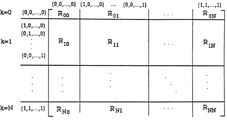
to be the set of all states 1B.. in which there are exactly i arrival proces~sin the busy state. Using this definition we can lump the state ,space int~ N

+

1 sets of

t t S · . - 0 1 2 l\T The transition matrix with the lumped states is shown In figure 4.

s a es

,,1 -

, , , ...,

j,y •

(1,1, ...,1)

(0,0, ... ,0) (1,0, ...,0) ... (0,0, ... ,1) (0,0,. .. ,0)

....

Roo

R

0 1

...

RON

-(11

°

1 . . .,0)

(0,1 ....,0) R

10 1<11

...

R_1N

(0/° /... /1)

(1,1" .., 1) RNO RNl

...

~NN

--

-k=l

k=N

k=O

Figure 4: The transition matrix with the lumped states

Let ~j be the transition probability from lump i to lump j. Then, we have

~;

=

L

Pr~fSi][

L

r(~

--.

w')],

~ESi !!!..ES;

(3)

where

and

Pr(SiJ

=

L

Pr(wJ.

!!ES,

Seeing that the N arrival processes are independent from each other, we have that

Pr[!!!J

=

Pr[wIJ·

Pr(w2] ...

Pr(wN],

where

1 - Pi

Pr[Wi

=

0]

=

2 ( )'

- Pi

+

qi

and

1 - qi

Pr[Wi

=

1]

=

2 ( ) ·

Thus, we have

p"U£j

=[

II

1 - Pi ][

II

1 - qi ]

. 2 - (Pi

+

q.). 2 -

(no

+

q.) ,

,ew

o

',ew

t ~ I

where for a given state ~ Wo and W1 are the sets of the arrival processes which are in the idle

state and the busy state respectively.

The generation of the aggregate transition matrix (hereafter denoted as A) is a time con-suming operation because we first have to generate the transition matrix associated with the N

arrival processes and subsequently calculate the transition probabilities ~;, i,

i

=

0, 1,2, ... ,N.

The computational effort for the generation of the aggregate matrixA can be significantly reduced by observing that the parameterspandqof a bursty ffiP process are very likely to be close to 1. For instance, in the case of voice, the squared coefficient of variation of the inter-arrival time

C2 is 18.1(see Heffes and Lucantoni [8]). Assuming a linkutilization of 0.1, and using equation(l) and (2), we find that p

=

0.922 and q

=

0.991. The higher the value of C2 , the closer to 1 p

and q get. It is highly unlikely, therefore, that a bursty source will change its current state at the next slot, seeing that 1 - p ~ 0 and 1 - q ~

o.

Based on this argument, we neglect all the transitions where more than two arrival processes change their statesinthe next slot. This results

ingreat savings when it comes to generate the transition matrix of the N arrival processes. As it will be seen in the validation section, neglecting these transtions does not affect the accuracy of the results. The structure of the non-zero elements of the resulting aggregate matrix A is shown

in figure 5. Finally, we note that further computational savings can be achieved using some of the combinatorial expressions givenin Iscoe, McDonald, and Qian [9].

3.2 Analysis of a subsystem

As it was mentioned earlier on, we analyze the queueing system. under study by decomposing it into N subsystems, one per queue. Inthis section, we describe how a subsystem is analyzed. The subsystems are combined together using the iterative procedure described in section 3.3.

Let us consider the

ith

queue. The remaining queues

will

be denoted by the symbol

N - {i}. In order to study the ith queue in isolation, we need to know how many cells are in N -

{i}.

Consequently, we analyze queue i by studying a subsystem of the original queueing system which consists of the following:

(a)

the arrival stream characterized by the superposition process,

(b)

queuei, and (c) the number of cellsin

N -

{i}. The queueing structure of a subsystemi

is showninfigure 6. The state of a subsystemi is given by the vector

(Ie,

n;,

n),

where

Ie

is the state of the superposition process, 11; is the number of cellsinthe ith queue, and n is the number of cells

in the entire system, Le., n -

na

is the number of cellsin the remaining queues N -

{i}.

The total number of states in the subsystem is (N+l)(M:ll(M+2). The synchronization of the departures and arrivals in a subsystem is the same as in the original queueing system. This is shownin figure 3. For presentation purposes, we shall refer to time t as being immediately after the end of slut t,

a

1 2 3 4 5 N-2

N-l

N

a

Roo

R

_{0 1} R_{0 2}

1 R10 R1 1

R

₁₂ R₁₃ 2 R_{2 0} R_{2 1} R₂₂ R₂₃ R₂₄

3 R3 1 RJ 2 R33 R34 R~s

N-2

N-l

N

RN-2JN'~ RN-2JN~ R11'-2 11'-2_I RN-2 11'- 1_I RN-2JN' Rli- 1,N-3 RN'-l,N-2 RN- 1,N'- 1Rlr-1, N'

RN',N-2 RN, lf- l R_NN

Figure 5: Aggregate transition matrix A

The automatic generation of the states of a subsystemis not discussed here since it is a straight-forward procedure, Below, we describe how the one-step transition probabilities are calculated. A one-step transition from state

(Ie,

n;, n) to state

(k',

n~,

n')

takes placeinsubsystemi ifone or more of the following events occur:

1. state change ofthe arrivalprocess

2. cell arrivals to queue i

3. cell arrivals to N -

{i}

4. cell departures from queue i

5. cell departures

from

N -

{i}

In case

(1),

the state of the arrival process is described

by

the number

Ie

of the arrival processes which areinbusy states. The transition probabilityfrom le to lei is

Riel.'

andit isgivenby

expression (3). Let us consider now cases

(2)

and (3). Since there are Ie arrival processes which are

Queue

i

m-o ·

Figure 6: Queueing structure of subsystem i

routed to output port i, We assume that every cellhas the same branching probabilities regardless of the input port at whichit arrived. Thus, with probability bi' ,where bi= L~lbji' an arriving cell joins the ith queue. In case

(4),

a cell always depart at the end of a slotifqueuei is not empty with probability 1.

In case (5), the number of cells that depart from the remaining queues N -

{i}

depends on how manyof these queues are busy. From the state description

(k,

Tti,n), we only know that there are n - TIi cells in N - {i}. We do not know how these cells are distributed over the N -

{i}

queues. For instance, all the cells could be in the same queue. In this case, only one cell will depart at the end of the next slot. On the other hand, allN - 1queues may contain at least one cell (provided that n - TIi

>

N - 1).

In

this case, there will be N - 1 departures. In order to calculate the transition probabilities out of state

(k,

11.&,n) due to cell departures from

N -

{i}, we use the probability distributionP~(l)that there are1busy queues in N -

{i},

given that there are

a,

=

n - 11; cells in N - {i}. This probability is obtained approximately as follows.

As it will be described below in section 3.3, at each iteration we will have an estimate of the mean number of non-empty queues, !i(ai), in N -

{i}

for subsystemi, given that there are

a,

cells in

N -

{i}. For eachai,

a.a

=

1,2, · · .,

M,

the unknown probability distribution

Pat (I)

satisfies the following constraints:

N-l

L

Pa.(l)

=

1

l=1

N-l

L

IPa,(I)

= !,(ai),

l=l

where we assume that PQ.i(I)

=

0 ifI

>

<li.

(5)

(6)

Since only the first moment of the probability distribution is given, there is an infinite number of probability distributions that satisfy constraint (5). We choose a distribution whose first moment matches

f,(aa)

using the notion of maximum entropy (see Kouvatsos and Xenios

[11]

and the references

within).

The maximum entropy distribution is the distribution that maximizes the entropy function

Lf:l

1PQ.i(I)ln(Pa,(I))subject to constraints

(4)

and (5). Using the method of the Lagrange's undetermined multipliers we obtain:

( _ 1 -l~

P01

1) -

Ze ,

where Z is the normalizing constant given by

Z

=

e-AJ

=

e-~

+

e-2fj

+... +

_{e-NfJ , (7)}

and

f30

is the Lagrange multiplier associated with the normalizing constraint (4). It can be easily shown that the Lagrangian multiplyer{3 satisfies the following relation:

8{3o

-8if

=

!i(Oi). (8)

f3

is determined from equation

(8)

numerically. Therefore, the probability distribution,Pa.(l), can be obtained using eqations

(6), (7)

and (8).

The algorithm that computes the transition probability from (k,11.&,n) to _(k',n~,nl),

Pr{(k,

n;,n) -+

(k',

n~,

n'l},

is summarized below. We use the following notation:

a.a

and aRare the number of cells that arrive at queuei andN -

{i}

respectively,aN is the number of cells that enter the whole system without blocking,nR is the number of cells in N -

{i} ,

d;anddR are the number of cells to depart from queue i and N -

{i}

respectively. All random variables are considered at time t except

nR'

and

ak

which are considered at the time t

+

1.

Algorithm

step 1:

a.a

=

n~

+

d; - Bi, whered; is 1 if queue is non-empty, 0 otherwise. step 2: FordR

=

1 to Min(N-l,nR)

begin

a~

=

n~

+

dB - nB

if

a.a

+

aR

=

Ie

(if

cells are not blocked) then

Pr{(k,

Tti,

n) - (k',

n~,

n/)}

=

Rlcl.,Pr{dR}[ (

~

)

bri(l -

bdl.-

a i] .

if~

+

aa

<

Ie

(if

cells are blocked) then

(9)

+ (

_a;k

+

_{l '})

b~+1(1

_ b-)Ja-Goi-l_,

~----'-,o-""~---'-end;

Once the transition probability matrix is set up, the stationary probability vector is obtained numerically.

3.3

The Iterative Procedure

Each subsystem i is analyzed in isolationifwe know the mean number afnon-empty queues

fi.(a,,)

in N - {i}, given that there are eli cellsin N - {i}. The results obtained fromall the subsystems are combined through an iterative procedure. Each iteration involves the solution of the N subsystems

inisolation. At the end of each iteration a convergence test is carried out.

If

the procedure has not converged the values of

!i(at),

a ..

=

1,2,···,M, i

=

1,2,···,N, the values of fi(a .. ) are adjusted and another iterationis carried out. Foreachsubsystemi, fi(a.. ) satisfies the following conditions:

1. fi(l) = 1

2.

fi(a..

+

1)

>

fi(O-i),

eli=1,2,... ,M

3.

fi(a..

+

1) -

I,(at)

>

li(01

+

2) -

1,(01

+

1)

4. 1,(Qi)

<

min(n - 1,Qi]

fi(a.a)

is calculated as follows. Let 9,(a.. ) be the mean number of non-empty queues in

queue

N -

{i}

when Cli cells arrive at the entire queueing system assuming that the service time at eachqueue is infinite. gi(

at)

is an upper bound of fie a .. ), and it is givenby the following expression.

n ~n

gi(

ao)

=

L

[1 -

(L-i:

1.i:i:1

P~

lao].

l=l,l;ei

L:;=l'J~'

p,

where Pi is the average arrival rate of the jth arrival process (given by expression (1)). Clearly 1~

fiCa,)

~

gi(a .. ). fi(a,)

is approximated as follows:

wh~e

0

~

{J

~

1. Note that

9i(at)

satisfies the above four conditions, and so does

fi(at,f3).

We

es~rm~te

fi(at)

iteratively by adjusting{Jup and down accordingly in order to meet a convergence

criterion,

In this study, we use the mean number of cells in the entire queueing system as a conver-gence criterion because it is computationally simple. Since we obtain the stationary probabilities

Pi(.c,

7J.i,

n)

for each subsystem i, the mean number of cells in the entire queueing system can be computedin the following two different ways:

N M

L L

n.aPi(n;)

&=1 ",,=1

(11)

(12)

where

Pi(1li)

is the marginal probability that there are

n.a

cells in the ith queue, and

Pi(n)

is the marginal probability that there are n cells in the entire queueing system as calculated from subsystem i. These two probabilities areobtained as follows:

N M

Pi(1li)

=

L L

PiCk,fli, n),

M=On=nt

and

N n

Pi(n)

=

L L

PiCk,fli,n).

1&=0"i=0

Convergence occurs

if

lEt - E21~ E. Ifconvergence has not occured, we adjust {3 and do another

iteration. Inparticular, we note thatE1 - E2is a monotonically increasing function of

1,(0-\).

Thus,

we can decide whether the 1;,(01) is overestimated or underestimated depending on

which

mean value is larger, and accordingly change

li(01)

in order to reduce the difference

E

1 and

E

2 - Below,

we summarize the approximation algorithm. The superscript, denotes the iteration number.

Algorithm

step 0: Set {3~

=

0 and

[3JI

=

1and .s

=

0

step 1: .s =.1

+

1,

13ft

=

(,L3~-1

+

J3f-l)/2

and calculate fiS(a,

13ft)

for a=l,...,M and

i=1,2,...

,N

using (9) and (10).

step 2: Calculate the probability distribution of nonempty queues,

Pat (I)

using

(6), (7),

and (8) for 1

=

1, 2, ... ,

N -

1.

. .

using the SOR method for i

=

1,2, ..., .LV.

step 4: Calculate

Er

and

Ei

using (11) and (12) respectively. step 5: If

IE

1 - E21 ~ E then stop.

if

E

1 -

E

2

>

Ethen set ,8~ =

13ft, 13i

=

13f-

1 and go to step 1.

if

E

1 -

E

2

<

-E then ,8~= f3~-1,

f3Z

=

13ft

and go to step 1.

Due to the nature of this iterative procedure it is possible that the quantities li(Qi)may converge before lEI - E21

<

E. Inthis case, no further improvement on the approximation results can

be achieved. Consequently, for convergence it is important to also check if fi(Oi) have converged.

In

order to simplify the convergence criteria, it was found emprically that it suffices to check ifthe absolute valueof the relativeerrorbetween

E

1 and

E

2 is less than e,i.e.

I

E"i

1

E,

I

~ _e.

4

Validation

The approximation algorithm was validated in two parts. Inthe first part, we checked the accuracy of the approximation method described in section 3.1 for constructing the superposition process.

In

the second part, we checked the accuracy of the entire approximation algorithm for analyzing the queueing model of the shared buffer switch showninfigure 2. All validations were carried out by comparing the approximate results against simulation data.

4.1

The Superposition Process

The accuracy of the superposition process was testedby analyzing an ATM multiplexer. Specifically, we considered a single finite capacity queue with N arrival process as shown in figure 7. Let B be the maximum capacity of the queue. The server is assumed to be slotted, and the service time is equal to 1 slot. Service begins and ends at slot boundaries. Each arrival stream is slotted, with a slot equal to a service time, and it is modelledby an

mp

with A

=

1 (Le. eachbusy slot contains a cell). The synchronization of the arrivals and the departures is shown in figure 3. Ifa cell arrives when the system. is empty, the cell waits until the beginning of the next service slot, and then begins its service. The cell departs one slot later.

The ATM multiplexer is analyzed using the techniques described in sections 3.1 and 3.2.

In particular, the N arrival processes are aggregated to a single superposition process with N

+

1

states. The finite capacity queue is then analyzed assuming that all arrivals are generated by the superposition process. The state of this system is given by the vector

(k, n),

where It: is the state of the superposition process, and n is the number of cells in the queue. (We note that the state space is a subset of the state space of the subsystem described in section 3.2) The system is observed immediately after the beginning of each slot. Ifit is found in state

(k, n),

then during the subsequent slot

Ie

arrivals will occur and at the end of the slot one cell will depart (given that

n

>

0). The transition probabilities

Pr{(k,

n) --.

(k', n')}

between two .;t~tes obtained using the transition probabilities ~; (see expression 3) of the aggregate matrix A. We have

IBP1~

:

DIIIDQ

~

IBP/

N

Figure 7: The ATM multiplexer

Wecan now solve numerically the system of linear equations

'E.,P

=

1!:where

P

=

Pr{(k,

n) ~

(le',

n')}, in order to obtain the steady state probabilities

?r(

k,n). In our experiments, we used the successive overrelaxation method to obtain

?r(

k,n). Once we have calculated the stationary vector

7r(k, n), we can calculate the probability distribution of the number of cellsin the queue P(n), and the probability P(r) that a cell will wait in the queue for r slots before it is transmitted. P(r) is

calculated as follows:

If we exclude the transmission time, every cell waits for a minimum of 0 slots and a maximum of B-1 slots. Let C; denote the expected number of cells which wait exactly r slots and

C

E denote the expected number of cells that entered the queue. Ifthe current state at slot i is (k,n), then k cells wouldarrivein thenext slot i

+

1. The number ofcellsin slot i

+

1is equal to the sum of the remaining cells and the new arriving cells, i.e., (n - 1)

+

k: Ifthis sum is less than the buffer size B, then alllc cells can enter the queue. However, ifit

is

greater than B, only the cells which the buffer can accomodate, i.e., B -

(n -

1),

can enter the queue, and the others arelost. Thus, CE is expressed as

B N

CE

=

L L

k1r(k,

n)

n=O Ie=l

where

k

=

min(k, B - (n -

1)).

Now, let us consider

C

p • Ifthe queue is empty or it contains one cell and the number of arriving cells at the next slot is more than

r

(k

>

r),

then exactly one cell among the arriving cells will wait for r slots in the queue before transmission. Likewise, if there are already two cells in

follows:

1"+1 N

o.

=

L: L:

~(k,

n)

n=Ok=,.+l-n

where

n

=

maz(O,

n

-1).

The probability

P(r)

that a cell waitsexactly

r

slots before transmission can now be obtained by dividing C,. by CE. (Note that in this calculation we do not include the offset of the arrival boundary to the next service boundary.)

The results obtained for the ATM multiplexer using the above approximation method were validated against simulation. In figures 8 and 10, we give the approximate and simulation results for P(n) and P(r)respectively, assuming 16 arrival processes (N

=

16), and a buffer capacity of 32

(B

=

32). (The confidence intervals were not plotted because they were too small) The absolute errors (simulation-approximation) are given in figure 9 and 11. The arrival processes were set as follows: Pi = 0.03125, i=1,2,...,16, and

C!

=

C?

=

Cl

=

C1

=

50,

Ci

=

CJ

=

C1

=

Cl

=

100,

C~

=

el

a =

ell

=

Cl

2 = 200,

Cl

3 =

Cl

4

=

Cl

s

=

Cl

e

=

500. We observe that there is a good

agreement between the approximate and simulation data. Ingeneral, ithas been observed that the approximate results have a good accuracy. The accuracy seems to be affected by the variability in the C2 values of the arrival processes. (The squared coefficient of variation of the interarrival. time

C

2 is used in this paper as a measure of burstiness of an arrival process). For example, the accuracy of the approximate results will not be as good if the C2 _{values of the arrival processes}

range from 1 to 500, rather than from 50 to 500. Depending on the number of arrival processes, the construction of the aggregate matrix may be CPU intensive. This is because it requires the generation of the Markov chain of the N arrival processes, which may involve a large number of states.

CPU

complexity problems were encountered when N

>

20. The case of N

=

8 can run efficiently on a workstation. The case of N

=

16 required a mainframe system.

The approximation method for constructing the superposition process can be easily adapted to the case where each individual arrival processes is defined in continuous-time as an Interrupted

Poisson Process (IFP). In this case, the construction of the aggregate matrix A is not time-consuming as inthe discrete-time case. Heffes [7] considered the case of superposing heterogeneous arrival processes. In particular, Heffes constructs an M11PP approximation to the superposition of any number of different MMPP sources using a set of very simple expressions. In order to compare our method against Heffes' method, we considered a continuous-time version of the ATM multiplexer where eacharrivalstream is represented by a different IFP, and the server provides an exponentially distributed service time. We assumed 8 arrival processes and a buffer capacity of 16. Each arrival process had an average arrival rate of 0.5, and a peak arrival rate of 1. The squared coefficient of variation of the interarrival time of the arrival processes was set as follows:

Cl

=

200,

Ci

=

100, C~

=

80, CI

=

50, C~

=

40,

CJ

=

20, Cf

=

10, Ci

=

2. The total offered average traffic was

2:T:1 "\i

= 4. The service rate J.L was obtained from the ratio v =

2:T=l

Ail

JJ, which in our experiments was varied from 0.1 to 0.96.

Using Heffes' approximation, we obtained anMMPPapproximation to the superposition of the 8 arr ival processes. Subsequently, we analyzed the multiplexer numerically as an MMPP

IM/l

finite capacity queue. The results for the grade-of-service( GOS), expressed as 100(1-P~{celllo",",}),

and we also give simulation results. We note that our approach gives better estimates for GOS as 1/

increases. This is probably due to the fact that the aggregate matrix A contains more information regarding the superposition process than Heffes' MMPP. However, our approximation method is computationally more intensive.

4.2

The Shared Buffer Switch

In this section, we diSCUB8 the validation of the approximation algorithm describedin section 3 for the analysis of the shared buffer switch. The approximation algorithm was used to analyze an 8X8 and a 16 X 16 shared buffer switch. The approximation results were compared against simulation data. Representative results are summarizedin tables 2 to 5. Each table gives approximate and simulation results for the global queue-length distribution

P(

n), n = 0, 1, 2, · · · ,

M,

and for the queue-length distribution

P

1

(nt), nt

=

0, 1, 2, · · · ,

M,

of queue 1 which is the most heavily utilized

queue (hot spot). Approximate and simulation results for the mean number of cells, m.q.l.,inthe switch is also given. The absolute errors for

P(n)

and

P1(nt)

givenin tables 2 to 5 have been plottedinfigures 14 to 17 respectively. The parameters of the arrival processes are given in table

1.

In

general, the approximation algorithm gives good results. The approximation results for the queue-length distribution

Pi(

11.&) of each queue i seem to be slightly more accurate than the global queue-length distributionP(n). CPU complexity problems were encounteredwhen N

>

20. The case ofN

=

8 can be done efficiently on a workstation. The caseN

=

16 required a mainframe system.

5

Conclusions

In

this paper, we presented an approximation algorithm for analyzing a discrete-time queueing

model of the shared buffer ATM switch. The arrival process to each port of the switch was

as-sumed to be bursty, and it was modelled by an ffiP. The discrete-time queueing model was ana-lyzed approximatelyusing the notion of decomposition. The queueing model was decomposed into subsystems, and each subsystem was analyzed separately. The results from the subsystems w~e combined together through the means of an iterative scheme. In order to reduce the complexity of each subsystem, the arrival processes to the switch were aggregated to a single superposition process. Comparisions against simulation data showed that the approximation algorithm hasa

table 2 Pi

=

0.2,i

=

1, 2, · · · , 8;

C!

=

Cl

=

500,

Ci

=

C~

=

200,

Cg

=

C~

=

100,

C?

=

Cl

=

50;

bil

=

0.5,bi2

= ... =

bi5 = 0.1,bi6

=

0.05,bi7

=

bi8

=

0.025

table 3 sameas in table 2

table 4 Pi

=

0.2,i

=

1, 2, · · · , 16;

C!

= ···

= Ci

=

500,

Cl

= ··· =

Cl

=

200,C~ = · · ·

=

Cr2

= 100, C2 -13 - ••• -- C 2 - 50·16 - ,

bil

=

0.21, bi 2

= ··· =

bi 5

=

0.082,bi6 = · · · = Gig = 0.06,

bilO

= ··· =

bil3 = 0.041,bi14

=··· =

bi16

=

0.020 table 5 Pii and

Ci,

i = 1, 2, · · ., 16, same as in table 4;

bil

=

0.339,bi2 = · · ·

=

bi5

=

0.068,bi6

= ··· =

big

=

0.051,

bilO

= ···

= bi13

=

0.034,bi14

= ···

=

bilS

=

0.017

P(n)

0.8

i

0.6

0.4 ...

•

accroxrrnancn sirnulancn

0.2

r

10 20 30

Number of cetls n

Figure 8: Queue length distribution

40

0.04

0.02

'- 0.00

0

t::

u

~ -0.02

-

...,J

:.12

~ :-:

-0.04

-O.OS

.

a

1 0 20

Number of

cells

n

30 40

Figure 9: Absolute errors for the results in figure 8

0.5

r

-0.4 - - c -_• acproximaticn_simulancn

0.3 -P(r)

0.2

0.1

-40

I

10 20 30

Number of slots r

0.0

-t-!!!!!!!!!!!.~

....

~-~-~

...

--J

o

Figure 10: Cell delay distribution

0.01 . , . . . - - - .

0.00

-0.01

-0.02

-0.03

40

10 20 30

Number

or

slots r

-0.04 ..._ _- - . . - - -...--..---~-....--.----4

o

Figure 11: Absolute errors for the results infigure 10

110 T

-100

""

C C

90

c Henas

•

our acprox•

•

simulation 80

0.0 0.2 0.4 0.6 0.8 1.

a

v

Figure 12: Comparisons for grade-of-service( GOS)

1.

a

0.3

a.o

0.4

0.2

o---~"'---"""-""'''''''''''''--'-''''''''''''-'''-~'''''''''''

0.0 8

:1 Hetfes

,.

_{our acprcx,}

a

•

simulancn

~

~I ₄

~

:!

-

...

-~ 2

v

Figure 13: Comparisons for the mean queue-length

I

P(n)

approx. simul, n

0 .1666 .1608±.OO54 0 .3329 .3264±.OO65 1 .3004 .2999±.O061 1 .1993 .1971±.OO37 2 .0469 .0642±.0022 2 .0595 .O572±.OOll 3 .0640 .O572±.0013 3 .0509 .0480±.OOO7 4 .0501 .0452±.0007 4 .0501 .0445±.001O 5 .0419 .0408±.0011 5 .0599 .0524±.0011 6 .0406 .0410±.OO09 6 .0830 .0821±.OO24 7 .0462 .0476±.OOO9 7 .1067 .122S±.OO51

8 .2432 .2433±.OlO5 8 .0576 .O699±.OO25 cell Ioss .16 .20±.01

m.q.l 3.38 3.51±.0719

Table 2: Approximate and simulation results for P(n) and

P1(nl)

switch size: 8x8,buffer size=8.

0.02

m abs err p(n)

•

abs errp1 (n1)

""-0 _0.01

""-OJ

0)

-

~

0

U')

.c _0.00 co

1

a

8

4 6

Number of cells n

2

a

-0.01 .J-_...- ...

--...---T--.,.----,----'l...--. .

-,....~

n

I

P(n)

approz, simul.

0 .1640 .1591±.0054 0 .3143 .3092±.0066

I

1 .2741 .2150±.0064 1 .1774 .1154±.O034

2 .0316 .0528±.0016 2 .0413 .0455±.0011

3 .0525 .0460±.0012 3 .0366 .0355±.OOlO

4 .0401 .0341±.OOlO 4 .0294 .0280±.OO09

5 .0298 .0272±.OO07 5 .0246 .0234±.OOO7

6 .0243 .0228±.0006 6 .0214 .0203±.OO06

7 .0210 .0201±.OO06 7 .0195 .0188±.0008

8 .0190 .0182±.0007 8 .0185 .017S±.OO05

9 .0178 .OI72±.OOO6 9 .0184 .0172±.OOO7

10 .0173 .0165±.OO07 10 .0193 .0176±.OO07 11 .0173 .0172±.0007 11 .0220 .0190±.OO07 12 .0181 .0182±.0005 12 .0281 .0229±.OO08 13 .0197 .0202±.0008 13 .0402 .0331±.OO10 14 .0230 .0240±.0009 14 .0605 .0625±.0035 15 .0299 .0320±.0012 15 .0795 .0977±.0057 16 .1945 .1993±.0121 16 .0433 .0564±.0032 cell loss .139 .148±.OO8

m.q.l 5.97 6.21±.16

Table 3: Approximate and simulation results for P{n) and

P1(nt)

switch size: 8x8, buffer size=16.

0.02

1:1 abs errp(n)

•

abs errp1 (n1)

\0- 0.01

0

\0-Q)

s

.a

0

en _0.00

..c ~

20

1 0

Number of cells n

a

-0.01 .J-_---r----r---...---~

n

I approx.

P(n) simul.

0 .1852 .1978±.0087 0 .6738 .6861±.OO83 1 .3264 .3364±.OO88 1 .2319 .2265±.OO41

2 .2025 .2341±.0053 2 .0541 .O508±.O024

3 .1399 .1143±.0048 3 .0170 .O156±.OO14 4 .0673 .0548±.O034 4 .0078 .O071±.0008

5 .0332 .0254±.0022 5 .0044 .O038±.0004 6 .0162 .0128±.001S 6 .0029 .0024±.0003 7 .0089 .0073±.0010 7 .0020 .OO17±.OO03 8 .0055 .OO4S±.OO05 8 .0015 .0014±.OO03 9 .0037 .0029±.0003 9 .0012 .OO11±.0002 10 .0026 .0020±.OO03 10 .0011 .0010±.OOOl 11 .0020 .OOlS±.OO02 11 .0009 .0009±.0002 12 .0015 .0012±.OO02 12 .0007 .0008±.OO02 13 .0012 .0011±.OO02 13 .0002 .0005±.OOOl 14 .0010 .0009±.00O2 14 .0 .OO02±.O 15 .0009 .OOO8±.0002

15

.0 .0 ±.O 16 .0021 .0022±.0006 16 .0 .0 ±.O cell loss .00181 .00165 ±.00062

m.q.l 1.89 1.81 ±.06

Table 4: Approximate and simulation results for P(n) andPI

(nl)

switch size: 16X16,buffer size=16.

0.06 0.04

--0 0.02 \ \ -co ~ :J 0.00 0 (J) .c ~ -0.02 -0.04 0

l!I abs err p(k)

• abs errp1(n1)

1 0

Number of cells n

20

n

I

P(n)

approx. simul.

0 .0281 .O293±.OO23 0 .3684 .3719±.O132

1 .1083 .112S±.0078 1 .2487 .2474±.OO40

2 .1204 .1850±.OO83 2 .1110 .lO82±.OO17

3 .1450 .1649±.O049 3 .0571 .0553±.OO15

4 .1219 .1187±.OO26 4 .0374 .0351±.OOI6

5 .0979 .O815±.OO17 5 .0286 .0261±.OO14

6 .0721 .0546±.OO14 6 .0242 .0215±.OO12

7 .0534 .O382±.OO17 7 .0222 .O193±.OO16

8 .0403 .O291±.OO15 8 .0215 .0183±.OO18

9 .0316 .O234±.OO14 9 .0213 .O188±.0020

10 .0258 .0199±.0014 10 .0204 .O196±.0018 11 .0221 .OI72±.OO14 11 .0174 .0203±.OO21 12 .0197 .0156±.OO14 12 .0122 .O180±.0018

13

.0183 .0146±.0015

13

.0065 .0127±.OOI4 14 .0174 .0146±.OOI3 14 .0023 .0059±.OOO8

15

.0166 .OI58±.OOI3 15 .0005 .0015±.OO02

16 .0602 .0651±.0071 16 .0 .OOO2±.O

cell 1088 .039 .O31±.03 m.q.l 5. 5.15±.20

Table 5: Approximate and simulation results for P(n) andPi

(nl)

switch size: 16

X

16, buffer size= 16.

m abs err p(n)

• abs errp1 (n1)

10 20

Number of cells n

Figure 11: Absolute errors for the results in table 5

0.08

0.06

~

0

~ ~

0.04

Q.) Q.)

'S 0

0.02

en

.!J

ca

0.00

References

[1] S. L. Albin, "Approximating a point process by a renewal process, 2: Superposition arrival processes to queues," Opere Re6.,32(5):1133-1162, 1984.

[2] A. Baiocchi, N. Melazzi, M. Listanti, A. Roveri, and R. Winkler, "Loss performance analysis of an ATM multiplexer loaded with high-speed on-off sources," IEEEJ. SA C,9:388-393, 1991.

[3] P. Boyer, M.R.Lehnert, and P.J. Kuehn. Queueinginan ATM basic switch element. Technical R.eport CNET-123-030-CD-CC, CNET, France, 1988.

[4]

H. Bruneel and B. Steyaert. Tail distribution of shared buffer queue contents. Technical report,

RUG Internal Research Report, Nr. 4, 900522.

[5] M. Devault, J.-Y. Cochennec, and M. Servel, "The "Prelude" ATD experiment: Assessments and future prospects," IEEE

J.

SAC, 6(9):1528-1537, December 1988.

[6] A. E. Eckberg and T.-C. Hou, "Effects of output buffer sharing on buffer requirements in an ATDM packet switch," INFOCOM '88, pp. 459-466, March 1988.

[7]

H. Heffes, "A class of data traffic processes-covariance function characterization and related queueing results," Bell Sys. Tech. J., 59:897-929, July-August 1980.

[8] H. Heffes and D. M. Lucantoni , "A Markov modulated characterization of packetized voice and data traffic and related statistical multiplexer performance," IEEE

J.

SA C, 4:856-868,

September 1986.

[9J

I. Iscoe, D. McDonald, and K. Qian. Capacity of ATM switch. Technical report, Dept. Math., Univ. of Ottawa.

[10] F.P. Kelly. Reversibility andStochastic Netuiroks. John Wiley & Sons, Inc., 1979.

[11] D.D. Kouvatsos andN.P.Xenios, "MEM for arbitrary queueing networks with multiple general services and repetitive-service blockings," Perform. Eval., 10:169-195, 1989.

[12] H. Kuwahara, N. Endo, M. Ogino, and T. Kozaki, "A shared buffer memory switch for an ATM exchange," Int. Coni. on Communications, pp. 4.4.1-4.4.5, Boston, MA, June 1989.

[13] H. Lee, K. Kook, C. S. Rim, K. Jun, and S.-K. Lim, "A limited shared output buffer switch for ATM," Fourth Int. Coni. on Data Communication Systema and Their Performance, pp. 163-179, Barcelona, 1990.

[14]

R.

Nagarajan,

J.

F. Kurose, and D. Towsley,"'Approximation techniques for computing packet loss in finite-buffered voice multiplexers," IEEE

J.

SAC,9:368-377, 1991.

[15]

I.

NOITos,

J.

W. Roberts, A. Simmonian, and

J.

T. Virtamo, "Loss performance analysis of an

ATM multiplexer loaded with high-speed on-off sources," IEEE J. SA C, 9:378-387, 1991.

[16] H. G. Perros and

R.

Onvural, "On the superposition of arrival ?rocesses for voice and data," Fourth

Int. Coni.

on Data Communication Systems and Their Performance, pp. 341-357,

[17] G.R. Petit, A. Buc.hheister, A. Guerrero, and P. Parmentier, "Performance evaluation methods applicable to an ATM multi-path self-routing switching network," Jensen and Iversen (Ed.),

Teletraffic and datatraffic in a period of change, pp. 917-922 North Holland, 1991.

[18]

G.H.

Petit and E. M. Desmet, "Performance evaluation of shared buffer multiserver output queue switches used in ATM," 7th ITCSpecialist Seminar, pp. paper 7.1, New Jersey, 1990.

[19] G. Pujolle and R.G.Perras, "Queueing systems for modelling ATM networks," Intrz coni. on the Performance of Distributed Sy,teTTU and Integrated Comm. Networks, Koyto, September 1991.

[20] B. Sengupta, "A queue with superposition of arrival streams with and application to packet voice technology," King, Mitrani,and Pooley(Ed~),Performance '90,pp. 53-59North Holland, 1990.

[21] K. Sriram and W. Whitt, "Characterizing superposition arrival processes in packet multiplexers for voice and data,"

IEEE

J.

SA

C, 4:833-846, September 1986.

[22] F.A. Tobagi, "Fast packet switch architectures for broadband integrated services networks," Proc.

IEEE,

78:1133-1167, January 1990.

[23] W. Whitt, "Approximation a point process by a renewal process, 1: Two basic methods," Opere tu«, 30(1):125-147, 1982.