Assessing the Value of Model Calibration for Signalized Intersection

(1)

ABSTRACT

Jiong Lin. Assessing the Value of Model Calibration for Signalized Intersections. (Under the

direction of Dr. Nagui Rouphail.)

The Highway Capacity Manual (HCM) provides the most widely used methodologies for

evaluating the quality of service on highway and street facilities. However, many users contend that the HCM models they are using are not accurate in emulating some real world conditions. In this thesis, the HCM control delay model for signalized intersections is assessed to identify where and when such deficiencies occur.

Four signalized intersections within the Chicago central business district (CBD) area are selected

to assess the accuracy of the HCM control delay model. The lane groups studied include three

through lane groups and one permissive left-turn lane group. Input data (e.g. lane group volumes,

proportion of vehicles arriving on green, effective green time, etc.) for the HCM model and

empirical data (e.g. actual measured control delay) were collected cycle by cycle in the field.

Saturation flow rates estimated from (a) the HCM default parameter values, (b) field calibration

and (c) statistical optimization are entered into the HCM control delay model, respectively, to

calculate control delays. Then, the control delays calculated from the model are contrasted to

those measured from the field.

For the through lane groups, the analysis indicates that the control delay calculated using the

(2)

from field measurements, and this indicates that the HCM control delay model is reliable. For the

(3)

ASSESSING THE VALUE OF MODEL CALIBRATION

FOR SIGNALIZED INTERSECTIONS

by JIONG LIN

A thesis submitted to the Graduate Faculty of North Carolina State University In partial fulfillment of the requirements for

The Degree of Master of Science

CIVIL, CONSTRUCTION, AND ENVIRONMENTAL ENGINEERING

Raleigh, NC 2004

APPROVED BY:

Dr. Joseph E. Hummer Dr. Billy M. Williams

Dr. Nagui M. Rouphail Chair of Advisory Committee

(4)

ii

BIOGRAPHY

Jiong Lin was born in Beijing, China. After graduation from Northern Jiaotong University in

Beijing, China, where she received a Bachelor of Science degree in Transportation Engineering

in July 1995, she worked for Civil Aviation Management Institute of China as an assistant

professor for eight years. In September 2001, she received her Master of Business Administration

(5)

iii

ACKNOWLEDGEMENTS

Many people have assisted me in the completion of my graduate thesis. I would first like to

acknowledge Dr. Nagui Rouphail, my academic advisor, who had spent a lot of time and spirits

with me on the thesis structure formulation, provided guidance on research materials. His

constructive and most helpful comments on my thesis draft deserve to be sincerely appreciated.

I would also like to thank Dr. Joseph Hummer and Dr. Billy Williams for serving on my thesis

committee and giving suggestions for ways to improve my research.

Last, I would like to thank my husband, Xuejun, for his understanding and support. Without his

(6)

iv

List of Tables

Table 3.1 Summary of Fixed Input Data for Studied Lane Groups... 32 Table 3.2 Summary of Average Saturation Flow Rates ... 33 Table 3.3 Summary of Control Delay Statistics ... 35 Table 4.1 Summary of Saturation Flow Rates, kI-values and Corresponding Control Delay MSEs by

Different Methods... 37 Table 4.2 Comparison of Control Delay MSE Using the HCM Default Saturation Flow Rate and kI

with/without Default Arrival Type ... 39 Table 4.3 Comparison of Control Delay MSE with Field Calibrated Saturation Flow Rate

and/or kI... 39 Table 4.4 Maximum Difference (sec) at Specified Assurance Levels for the Southbound Through

Lane Group at Wells-Grand Intersection... 45 Table 4.5 Maximum Difference (sec) at Specified Assurance Levels for the Southbound Through

Lane Group at LaSalle-Ohio Intersection... 50 Table 4.6 Maximum Difference (sec) at Specified Assurance Levels for the Northbound Through

Lane Group at LaSalle-Ontario Intersection... 56 Table 4.7 The Optimal MSEs and Corresponding Saturation Flow Rates (veh/h/ln) and kI Values for

the Two Study Periods at LaSalle-Ontario Intersection ... 57 Table 4.8 Summary of Sensitivity Analysis for the Control Delay MSE for Cycles 29 through 48

at LaSalle-Ontario Intersection... 59 Table 4.9 Maximum Difference (sec) at Specified Assurance Levels for the Northbound Permissive

Left-turn Lane Group at LaSalle-Ontario Intersection ... 65 Table 4.10 Comparison of Control Delay for Cycle 18 and Cycle 45 ... 67 Table 4.11 Comparison of Control Delay Using 5-minute Data for the Northbound Permissive

Left-turn... 68 Table 4.12 Statistical Relationship between Control Delay Estimated Using the HCM Model and the

Field Measurements for Through Lane Groups... 72 Table 4.13 Statistical Relationship between Control Delay Estimated Using the HCM Model and the

Field Measurements for Permissive Left-turn Lane Groups... 75 Table A.1 Summary of Field Measurements for Southbound Through Lane Group

at Wells-Grand Intersection... 83 Table A.2 Summary of Field Measurements for Southbound Through Lane Group

at LaSalle-Ohio Intersection ... 84 Table A.3 Summary of Field Measurements for Northbound Through Lane Group

at LaSalle-Ontario Intersection... 85 Table A.4 Summary of Field Measurements for Northbound Left-turn Lane Group

(9)

vii

Table C.1 Summary of Control Delay (sec/veh) for Southbound Through Lane Group at Wells-Grand Intersection... 90 Table C.2 Summary of Control Delay (sec/veh) for Southbound Through Lane Group

at LaSalle-Ohio Intersection ... 91 Table C.3 Summary of Control Delay (sec/veh) for Northbound Through Lane Group

at LaSalle-Ontario Intersection... 92 Table C.4 Summary of Control Delay (sec/veh) for Northbound Permissive Left-turn Lane Group

at LaSalle-Grand Intersection ... 93 Table D.1 The Control Delay Estimated by the HCM Model Using the Cycle-by-cycle Saturation

(10)

viii

List of Figures

Figure 3.1 Wells-Grand Intersection Configurations and Signal Timing Plan... 26

Figure 3.2 LaSalle-Ohio Intersection Configurations and Signal Timing Plan... 28

Figure 3.3 LaSalle-Ontario Intersection Configurations and Signal Timing Plan ... 30

Figure 3.4 LaSalle-Grand Intersection Configurations and Signal Timing Plan... 31

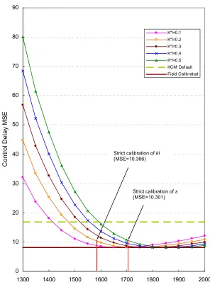
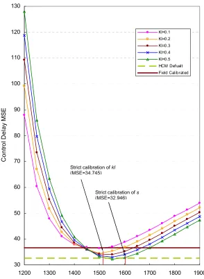
Figure 4.1 Control Delay MSE vs. Saturation Flow Rate, s, and Parameter, kI, for the Southbound Through Lane Group at Wells-Grand Intersection ... 41

Figure 4.2 Comparisons of Control Delay for the Southbound Through Lane Group at Wells-Grand Intersection... 42

Figure 4.3 Distributions of Control Delay for the Southbound Through Lane Group at Wells-Grand Intersection... 43

Figure 4.4 Distributions of LOS for the Southbound Through Lane Group at Wells-Grand Intersection ... 44

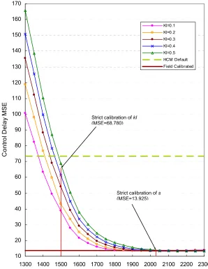
Figure 4.5 Control Delay MSE vs. Saturation Flow Rate, s, and Parameter, kI, for the Southbound Through Lane Group at LaSalle-Ohio Intersection ... 47

Figure 4.6 Comparison of Control Delay for the Southbound Through Lane Group at LaSalle-Ohio Intersection ... 48

Figure 4.7 Distributions of Control Delays for the Southbound Through Lane Group at LaSalle-Ohio Intersection ... 48

Figure 4.8 Distribution of LOS for the Southbound Through Lane Group at LaSalle-Ohio Intersection ... 50

Figure 4.9 Control Delay MSE vs. Saturation Flow Rate, s, and Parameter, kI, for the Northbound Through Lane Group at LaSalle-Ontario Intersection ... 53

Figure 4.10 Comparisons of Control Delay for the Northbound Through Lane Group at LaSalle-Ontario Intersection... 54

Figure 4.11 Distributions of Control Delay for the Northbound Through Lane Group at LaSalle-Ontario Intersection... 54

Figure 4.12 Distribution of LOS for the Northbound Through Lane Group at LaSalle-Ontario Intersection... 55

Figure 4.13 Distributions of Control Delay for the Northbound Through Lane Group with Different Saturation Flow Rates at LaSalle-Ontario Intersection ... 58

Figure 4.14 Sensitivity Analysis of the Control Delay MSEs vs. Decrease of Proportion of Arriving on Green for Cycles 29 through 48 at LaSalle-Ontario Intersection ... 60

(11)

ix

Figure 4.16 Comparisons of Control Delay for the Northbound Permissive Left-turn Lane Group at LaSalle-Grand Intersection ... 62 Figure 4.17 Distributions of Control Delay for the Northbound Permissive Left-turn Lane Group

at LaSalle-Grand Intersection ... 63 Figure 4.18 Distributions of LOS for the Northbound Permissive Left-turn Lane Group

at LaSalle-Grand Intersection ... 64 Figure 4.19 Comparison of Control Delays Obtained from the HCM Model with Cycle-by-cycle

Saturation Flow Rate against Field Measurement ... 66 Figure 4.20 Comparison of Control Delay Estimated Using the HCM Model to the Field

Measurements for Through Lane Groups... 71 Figure 4.21 Comparison of Control Delay Estimated Using the HCM Model to the Field

(12)

1

CHAPTER 1. INTRODUCTION

1.1Background

The Highway Capacity Manual (HCM) published by the Transportation Research Board provides

traffic engineers and researchers alike with the most widely used methodologies for evaluating

the quality of service on highway and street facilities. It is the primary document presenting

methods for assessing capacity and level of service for elements of the surface transportation

system not only in the United States, but also in many other countries in the world. The first

edition of the HCM was published in 1950. The second and third editions were published in 1965

and 1985, respectively. The latest edition of the HCM was published in 2000.

A continuing concern about the HCM procedures is the following: are the models presented in

the HCM reliable enough and applicable to all highway and street facilities under a variety of

operating conditions? A sound model should reflect real world conditions. Many users contend

that the HCM models they are using are not accurate, and the models have some limitations in

emulating some real world conditions. While one cannot expect the models to fit all empirical

data, there is a need for a rigorous assessment of where and when such deficiencies occur.

1.2Problem Statement

By far, the most widely used chapter in the HCM is the signalized intersection analysis. In

particular the control delay model for signalized intersections is the key to estimate the level of

service (LOS) at all signalized intersections. A host of variables and parameters need to be input

to the model in order to calculate control delay. Some of the variables can be measured directly

from the field, such as intersection geometry, intersection signal timing, and lane group volumes,

(13)

2

values are typically used. Lane group saturation flow rate, one of the most important variables, is

a typical derivative variable that enters into the calculation of control delay. That variable is

derived from the functional relationship between an ideal saturation flow rate and several

adjustment factors including lane widths, heavy vehicle percentages, number of bus stops,

pedestrian volumes, number of parking maneuvers, etc.

The HCM recommends the use of a locally calibrated saturation flow rate wherever possible. The

implication is that a properly calibrated model will yield an acceptable delay estimate and

consequently a more realistic level of service. This assumption needs to be verified against field

observations. Since the delay model parameters including the saturation flow rate can be directly

observed in the field (e.g. demand, duration of the analysis period), it can be assumed that any

discrepancies between the observed and estimated HCM delay may be due to errors in the delay

model formulation itself.

1.3Objectives and Scope

The nature of traffic operations at signalized intersections may vary from site to site, such as

traffic flow, drivers’ characteristics, and intersection geometry, etc. The purpose of this research

is to assess the HCM 2000 control delay model for signalized intersections with various

un-calibrated and un-calibrated saturation flow rates. Input data (e.g. lane group volumes, proportion of

vehicles arriving on green, effective green time, cycle length, etc.) for the HCM model and

empirical data (e.g. actual measured control delay) are collected from the field. Saturation flow

rates estimated from (a) HCM formulae, (b) field calibration and (c) statistical optimization are

(14)

3

control delays calculated from the model are compared to the control delay measured from the

field. The following questions are to be answered at the end of this research:

• To what extent does the un-calibrated HCM saturation flow rate and corresponding delay

estimate adequately predict field delay at signalized intersections?

• What is gained, in terms of prediction power, by using a field calibrated saturation flow

rate and delay model parameters?

• What is the remaining error in predicting control delay when an optimal saturation flow

rate and delay parameters are used? and,

• Are there differences in delay estimation for through and permitted left-turn lane groups?

Four signalized intersections within Chicago central business district (CBD) area are selected for

this research. All signals selected are pre-timed. The lane groups being studied include three

through lane groups and a permissive left-turn lane group. Traffic data were collected cycle by

cycle during one-hour study period. Instead of peak 15-minute analysis period, the length of one

cycle is used as the unit of analysis period to estimate average control delay in the HCM control

delay model. Comparison and analysis of saturation flow rates, distribution of control delay, and

distribution of level of service (LOS) are conducted to evaluate the reliability and applicability of

the HCM 2000 control delay model.

1.4Organization

There are five chapters in this thesis. Chapter 1 is the introduction. Literature review is provided

in Chapter 2, which includes the HCM methodology and other methods of model calibration and

validation. Chapter 3 introduces the methodology that is employed in this research and a

(15)

4

lane groups, in which the assessment of the reliability of the HCM 2000 control delay model is

performed. In the final part, Chapter 5, uncertainties of the HCM 2000 control delay model are

(16)

5

CHAPTER 2. LITERATURE REVIEW

The HCM 2000 control delay model for signalized intersections is reviewed in this chapter.

Three methodologies for model calibration and validation are also reviewed. Koutsopoulos et al.

(2) summarize the general statistical methods to validate traffic models. Rouphail et al. (3, 4) use

microscopic simulation to assess a generalized delay model that is based on HCM 1994 delay

model. Sacks et al. (5, 6) apply a Bayesian methodology to calibrate and validate the HCM 2000 control delay model. The estimation of permissive left-turn capacity is much more complicated, which is effected by the opposing flow. Mousa et al. (7) discuss the effect of opposing platoon on permissive left-turn capacity.

2.1HCM Methodology

The HCM 2000 (1) defines control delay at signalized intersections as the average control delay

experienced by all vehicles that arrive in the analysis period, including delays incurred beyond

the analysis period when the lane group is oversaturated. The HCM 2000 control delay model for

signalized intersections includes three parts: uniform delay, incremental delay, and initial queue

delay. HCM 2000 (1) describes the average control delay per vehicle for a given lane group as:

3 2

1(PF) d d

d

d = + + Eq. (2.1)

where

d = control delay per vehicle (sec/veh);

d1 = uniform control delay assuming uniform arrivals (sec/veh);

(17)

6

d2 = incremental delay to account for effect of random arrivals and oversaturation queues,

adjusted for duration of analysis period and type of signal control; this delay component assumes that there is no initial queue for lane group at start of analysis period (sec/veh); and

d3 = initial queue delay, which accounts for delay to all vehicles in analysis period due to

initial queue at start of analysis period (sec/veh).

The progression adjustment factor is determined by the proportion of vehicles arriving on green.

Good progression means that most vehicles arrive on green and the average delay per vehicle is

low. On the other hand, with poor progression, most vehicles arrive on red and experience longer

delay at the intersection. The progression adjustment factor in HCM 2000 (1) is defined as:

) / ( 1

) 1 (

C g

f P

PF PA

− −

= Eq. (2.2)

where

P = proportion of vehicles arriving on green;

g = effective green time (sec);

C = cycle length (sec); and

fPA= supplemental adjustment factor for early and late platoons arriving during green.

The proportion of vehicles arriving on green may be either measured in the field or estimated

from arrival type.

2.1.1 Uniform Delay

The estimate of uniform delay in HCM 2000 (1) is based on the assumptions of uniform arrivals

(18)

7 ] / ) , 1 [min( 1 ) / 1 ( 5 . 0 2 1 C g X C g C d − −

= Eq. (2.3)

where X is the volume/capacity ratio or degree of saturation for lane group, which is given by:

sg vC c v

X = = Eq. (2.4)

where

v = demand flow rate for lane group (veh/h);

s = saturation flow rate for lane group (veh/h); and

c = capacity of lane group (veh/h).

X values beyond 1.0 are not applicable in the computation of uniform delay, but are transferred to the second delay term, d2.

2.1.2 Incremental Delay

As presented in HCM 2000 (1), the incremental delay accounts for non-uniform arrivals,

temporary cycle failures, and oversaturated flow conditions. HCM 2000 (1) defines incremental

delay as       + − + − = cT kIX X X T

d 900 ( 1) ( 1)2 8

2 Eq. (2.5)

where

d2 = incremental delay to account for effect of random and oversaturation queues,

adjusted for duration of analysis period and type of signal control (sec/veh); this delay component assumes that there is no initial queue for lane group at the start of analysis period;

T = duration of analysis period (h);

(19)

8

k = incremental delay factor that is dependent on controller settings and v/c ratio; and

I = upstream filtering/metering adjustment factor.

According to the definition given by HCM 2000 (1), the parameter k is included in the above equation to incorporate the effect of controller type on delay. For pre-timed signals, a value of k

= 0.5 is used, which is based on a queuing process (M/D/1) with random arrivals and uniform

service time equivalent to the lane group capacity. The incremental delay adjustment factor

accounts for the effects of filtered arrivals from upstream signals. The default value of I =1 is based on the assumption that arrivals each cycle follow a Poisson distribution so that the variance

in arrivals equals the mean. An I-value of less than 1.0 is used for nonisolated intersections. This reflects how an upstream signal could decrease the variance in the number of arrivals per cycle at

the subject intersection. Incremental delay is sensitive to the degree of saturation for lane group

(X). When X>1.0, the control delay increases dramatically.

2.1.3 Initial Queue Delay

When there is unmet demand at the end of an analysis period, where the volume/capacity ratio is

greater than 1.0, an initial queue occurs at the beginning of the following analysis period.

Vehicles arriving in this following time period inevitably experience additional delay since the

initial queue must first clear the intersection. In these cases, the initial queue delay must be

considered. HCM 2000 (1) estimates initial queue delay using the following equation,

cT t u Q

(20)

9

where

Qb = the initial queue at the start of period T (veh);

c = lane group capacity (veh/h);

T = duration of analysis period (h);

t = duration of unmet demand in T (h); and

u = delay parameter.

The parameters t and u are estimated by the following equations:

t = 0 if Qb = 0, else

      − = )] , 1 min( 1 [ , min X c Q T

t b _{, and}

u = 0 if t<T, else

)] , 1 min( 1 [ 1 X Q cT u b − − =

When there is initial queue, the computation of uniform control delay (d1) must be evaluated

using X = 1.0 for the period (t) during which the initial queue clear the intersection and using the actual X value for the remainder of the analysis period (T-t). In these cases, a time-weighted value of d1 is used, as indicated below,

T t T PF d T t d

d₁ = _s* + _u* *( − ) Eq. (2.7)

where

ds = saturated delay (i.e. d1 evaluated for X = 1.0); and

(21)

10

2.2General Statistical Validation Methods

Statistical methods are widely used in the process of model calibration and validation.

Comparisons between field observations and results from model calculations using statistical

methods give analysts significant confidence on whether the model is effective or not.

Koutsopoulos et al. (2) suggest that the selection of appropriate methods and their application for

validating traffic models depends on the nature of the output data. Single-valued measures of

performance (MOPs), for example, average delay, are appropriate for small-scale application in

which one statistic summarizes the performance of a traffic network system. Multivariate MOPs,

for example, time-dependent flow, capture the temporal and/or spatial distribution of a MOP to

describe the dynamics of a system. Three statistical approaches for model validation are

discussed.

• Goodness-of-fit measures

Statistics including root mean square error (RMSE), root mean square percent error

(RMSPE), mean error (ME), and mean percent error (MPE) can be used as

goodness-of-fit measures to evaluate the overall performance of traffic models.

RMSE and RMSPE penalize large errors at a higher rate relative to small errors. These

two measures are given by:

∑

= − = N n obs n n Y Y N RMSE 1 2 mod ₎ ( 1

Eq. (2.8)

∑

=      − = N

n nobs

obs n n Y Y Y N RMSPE 1 2 mod 1

Eq (2.9)

where Ynobs and Ynmodare the averages of observed and model estimated measurements at

(22)

11

ME and MPE indicate the existence of systematic under-prediction or over-prediction in

the model estimated measurements. They are given by:

∑

= − = N n obs n n Y Y N ME 1 mod ₎ ( 1

Eq. (2.10)

∑

=

−

= N

n nobs

obs n n Y Y Y N MPE 1 mod ₎ ( 1

Eq. (2.11)

ME and MPE are more useful when applied to measurements at each point in space than

to all measurements jointly.

Koutsopoulos et al. (2) state another measure, Theil’s inequality coefficient, U, which

provides information on the relative error. It is given by:

∑

= = = + − = N n obs n N n n N n obs n n Y N Y N Y Y N U 1 2 1 2 mod 1 2 mod ) ( 1 ) ( 1 ) ( 1

Eq. (2.12)

where U is bounded (0≤U≤1). U = 0 implies a perfect fit between the observed and modeled measurements. U = 1 implies the worst possible fit.

• Hypothesis testing and Confidence intervals

Besides the classic hypothesis tests, such as two-sample t-test, Mann-Whitney test, and

two-sample Kolmogorov-Smirnov test, Koutsopoulos et al. (2) recommend using test for

the equality of the mean of observed and modeled measurements, by which no

assumptions like normal distribution and/or equal variance are needed. The statement of

hypothesis is given as following:

(23)

12 _f obs obs obs t n s n s Y Y ˆ , 2 / 2 mod 2 mod mod ) ( ) ( ≥ α + −

Eq. (2.13)

where _Yobs,_Ymod,_sobs,_and_smod_{are the sample means and standard deviations of the}

observed and model estimated measurements, respectively. _nobs _and _nmod _{are the}

corresponding sample size. fˆ is the modified number of degrees of freedom, and is

given by: ) 1 ( ) ( ) ( ) 1 ( ) ( ) ( ˆ 2 4 mod 2 mod 4 mod 2 mod mod − + −       + = obs obs obs obs obs n n s n n s n s n s

f Eq. (2.14)

The corresponding (1-α) confidence interval is given by:

_obs obs f obs n s n s t Y Y 2 mod 2 mod ˆ , 2 /

mod ₎ ( ) ( )

( − ± _α + Eq. (2.15)

Koutsopoulos et al. (3) also discuss a regression procedure that can be used to validate

traffic models using an F-test of the joint equality of the means and variances of the field

and modeled measurements. Assuming there are N different input data sets, for pairs of

observations ( , mod),

n obs

n y

y n = 1, …, N, the following regression is performed:

obs _n _n

n n

obs

n y y y

y − )=

β

+

β

( + )+

ε

( mod

1 0

mod _Eq._(2.16)

The hypothesis that the observed and model outputs are drawn from identical

(24)

13

2.3Validation Using Microscopic Simulation Model

Usually, a comparison between field observed data and model calculated results is one of the

most effective methods to assess traffic models. In some cases, however, it is extremely difficult

to obtain field data due to various limitations, for instance, limited availability of funds. For

these cases, other methods may be used, from which the outputs are considered the same as or

very close to data obtained through field observation. Rouphail et al. (3, 4) propose a generalized

delay model for inclusion in the update of HCM 1994, where the TRAF-NETSIM microscopic

simulation model is used to verify this delay model for oversaturated conditions and for

vehicle-actuated traffic signals.

In this case, TRAF-NETSIM outputs were compared with field data for undersaturated conditions and were found to be in general agreement. A total of 180 scenarios were analyzed in Rouphail et al.’s research (3), and 20 replications were conducted for each scenario with different random-number seeds to obtain a reasonably accurate estimate of the average delay. Delay curves for analysis periods of 15- and 30-min for HCM 1994 delay model, generalized delay model, and TRAF-NETSIM simulation model were plotted together in a figure. The plot indicates that the generalized delay model corresponds closely to the simulated delay values, but the HCM model doesn’t. A conclusion is drawn that the proposed generalized delay model is more suitable than the HCM 1994 delay equation for use

under oversturated conditions.

For validating the generalized delay model for vehicle-actuated traffic signals (4), similar inputs

(such as traffic volumes, average queue discharge headway, and average signal timings) were

entered into TRAF-NETSIM and the generalized delay model. Delay values obtained from

(25)

14

performed and plots of TRAF-NETSIM delays against model estimated delays for all volume

levels and signalization alternatives were generated. The analysis and plots show that the mean

square error (mean of the squared difference between simulated delay and model delay) is low

and the slope of the regression line passing through the origin is close to 1.0. This indicates that

the generalized model delays and TRAF-NETSIM delays are comparable.

In addition, the delays calculated from the HCM 1994 delay model and the generalized model were compared with delay data collected from the field (4). Regression analysis indicates that the mean square error for the HCM 1994 delay model is almost twice of that for the generalized

delay model. The slope of the regression line passing through the origin for the generalized

model delays is closer to 1.0 than that for the HCM 1994 model delays. It is evident from the

mean square errors and slopes that the delay values estimated with the generalized model are

closer to values observed in the field than the delays estimated by the HCM 1994 delay model.

Since the generalized delay model and TRAF-NETSIM yield comparable delays and the

generalized model delays were comparable to field observed delays, a conclusion is drawn that

the generalized delay model is an improvement over the HCM 1994 delay model for estimating

delays at vehicle-actuated traffic signals.

2.4Bayesian Analysis

Bayarri et al (5) point out that a model is a biased representation of reality and accounting for this

bias is the central issue for model validation. Furthermore, models alone could not provide

evidence of bias. Either expert opinion or field data is necessary to assess the bias – they focus on

the latter. Let xi be the input and u be the tuning parameters. They statistically model “reality =

(26)

15 ) ( ) , ( )

( M _i _i

i

R _x _y _x _u _b _x

y = + Eq. (2.17)

When field data x1, x2, …, xn are obtained, the model is:

F i i i M F i i R i

F _x _y _x _y _x _u _b _x

y ( )= ( )+ε = ( , )+ ( )+ε Eq. (2.18)

where: yF and yM denote field and model outputs, respectively, yR(xi) the value of “real”

process at input xi, b(xi) the model bias which is an unknown function and treating it requires

non-standard techniques, and εiR the independent normal random errors with mean zero and

variance λF.

Batista Paulo et al. (6) used the Bayesian methodology in calibrating and validating the HCM

control delay model. The parameters that can be obtained by calibration through the use of field

data are classified into three categories: a) parameters that can be directly estimated, perhaps with

error, from field data; b) parameters not directly measurable; and c) tuning parameters that are

not “real” but are required by the model. According to this research (6), Bayesian analysis

provides an attractive path to simultaneously calibrate the parameters of type (a), (b) and (c) and

deal with the possible presence of model bias. Therefore, calibration and assessment of validity

can be done in one combined analysis. Bayesian analysis determines the posterior distribution of

model parameters and inputs, given the observed field data. The resulting distribution will then

reflect the actual uncertainty in the parameters and inputs, adjudicate between the tuning

parameters and the possible model bias thereby providing resistance to over-tuning, and quantify

and assess the model bias.

To predict the real process, yR_(x

i), Batista Paulo et al. (6) used the bias-corrected prediction to

verify the delay model. At given x,

[

]

∑

=

+

= N

n i i

M

R _y _x _u _b _x

N x y 1 ) ( ) , ( 1 ) (

(27)

16

Assuming u was the posterior mean of the tuning parameters, they defined the pure model prediction of reality with the estimate of the bias, bˆ(x), as

) ˆ , ( ) ( ˆ ) (

ˆ _x _y _x _y _x _u

b ₌ R ₋ M _Eq._(2.10)

Tolerable difference was also introduced to indicate if the model was reliable for the reality. The expression is stated as (6):

[

"reality"−prediction ≤

δ

]

>

α

Pr Eq. (2.21)

where δ is the tolerable difference, and α is the acceptable probability. For the bias-corrected prediction, the expression can be stated as (15):

[

( , )+ ( )− ˆ ( ) ≤

δ

]

>

α

Pr y x u b x yR x

i i

M _Eq._(2.22)

If δ is small enough within the probability α, the model is valid. If δ is greater than a tolerable value, the model may not be reliable.

2.5Effect of Opposing Flow on permissive Left-turn Capacity

The estimation of permissive left-turn capacity is much more complicated than that for through

movements, which not only depends on the conditions of the approach but also on the opposing

flow. Mousa et al. (7) indicates that the observed left-turn capacity is inversely proportional to

the platoon ratio and flow rate on the opposing approach, e.g. progression for through traffic may

have an adverse effect on the opposing permissive left-turns.

Left-turn data were measured in an exclusive left-turn lane which was opposed by one lane of

through traffic. Data were collected only from cycles when left-turn queues spilled over to the

next cycle (i.e. demand > capacity). They examined data through several regression models to

determine whether there was an effect of measured parameters on the permissive left-turn

capacity. The regression results showed that the estimate of the permissive left-turn capacity

decreased as opposing flow rate increased and good progression on the opposing approach

(28)

17

In addition, Mousa et al. (7) performed two analyses to validate the 1985 HCM left-turn capacity

estimation procedure with field data, the 1985 HCM procedure with default saturation flow rates

and the 1985 HCM procedure with saturation flow rates estimated from field observations. It was

found that the ratio of observed to 1985 HCM capacities decreased as progression of opposing

flow improved. This indicates that the 1985 HCM method may overestimate left-turn capacities

under these conditions relative to the poor progressive situations.

2.6Summary of Literature Review

The 2000 HCM control delay model for signalized intersection, which includes three terms,

uniform delay, incremental delay, and initial queue delay, is described in this chapter. Methods

for model calibration and validation are also reviewed. Koutsopoulos et al. (2) summarized a few

widely used statistical methods in the process of model calibration and validation, including

goodness-of-fit measures, hypothesis testing and confidence interval. Rouphail et al. (3,4) used

microscopic simulation model (TRAF-NETSIM) to validate a generalized delay model and the

1994 HCM control delay model for oversaturated conditions and for vehicle-actuated traffic

signals, because it was considered that the simulation model could reflect the field situations.

Batista Paulo et al. (6) applied the Bayesian methodology to calibrate and validate the HCM 2000

control delay model. Since the Bayesian methodology can simultaneously calibrate the particular

parameters and deal with the possible presence of model bias, the calibration and validation can

be done in one combined analysis. The data used in Rouphail et al.’s and Batista Paulo et al.’s

research for the HCM control delay model calibration and validation were collected from through

lane group only. The permissive left-turn situation was not considered. Mousa et al.’s (7)

(29)

18

improvement of progression on the opposing approach can cause a decrease of left-turn capacity.

Most of the studies reviewed are focused on the methodologies and procedures of the HCM delay

model calibration and validation. However, there is no published research on assessing the value

(30)

19

CHAPTER 3. METHODOLOGY AND DATA

This chapter describes the methodology employed in this research to assess the HCM control

delay model. Various un-calibrated and calibrated saturation flow rates are used in the HCM

delay model to calculate model delays, and the model delays are then compared with field

measurements. Data collection for four selected lane groups is described, including intersection

configuration, traffic volume, signal display, and so on.

3.1Method Description

In the HCM control delay model for signalized intersections, the input parameters, including

cycle length (C), effective green time (g), analysis period (T), traffic flow rate (v), proportion of vehicles arriving on green (P), and initial queue (Qb), are measured directly from the field. Cycle

length (75seconds) is used as the duration of analysis period (T) instead of the 15-minute period that is used in most other studies using the HCM methodology, since the measurement of average

field delay in this research is based on cycle by cycle measurements.

The degree of saturation (X) is determined by lane group saturation flow rate (s) because g and C

are fixed for pre-timed signals. The HCM procedure uses the default ideal saturation flow rate

with considerations of adjustments for other factors to compute the lane group saturation flow

rate. It may or may not reflect the field situation. The alternatives use field calibrated and

statistically optimized saturation flow rates.

In the incremental delay (d2) equation, the incremental delay factor (k) and upstream

filtering/metering adjustment factor (I) are difficult to directly measure in the field. Because k

(31)

20

Then, the HCM control delay model can be described as (see Section 2.1 for definitions of the parameters): ) ( 1 ) 1 ( ) ( C g f P P PF PA − −

= Eq. (3.1)

    _      − − = − − = C g sg vC C g C C g X C g C s v d ,. 1 min 1 ) 1 ( 5 . 0 ] ) , 1 [min( 1 ) 1 ( 5 . 0 ) , ( 2 2

1 Eq. (3.2)

      + − + − = cT kIX X X T kI s v

d ( , , ) 900 ( 1) ( 1)2 8

2 Eq. (3.3)

cT t u Q s Q v d b b ) 1 ( 1800 ) , , ( 3 +

= Eq. (3.4)

where v, P, Qb are input variables for the model, and they change from cycle to cycle. s and kI

are the two tuning parameters in the HCM delay model and they are assumed to be constant for individual intersections during the one-hour study period. The total control delay in the ith

cycle with no initial queue presence (Qb = 0) is given by

) , , ( ) ( ) , ( ) , , ,

(v P s kI d₁ v s PF P d₂ v s kI

dModel _i _i ₌ _i _i ₊ _i _Eq._(3.5)

The total control delay in the ith_{cycle where an initial queue is present (}_Q

b>0) is given by

) , , ( ) , , ( ) ( ) , ( ) / 1 ( 5 . 0 ) , , , ,

( _, ₁ d₂ v skI d₃ v Q_, s T t T P PF s v d T t C g C kI s Q P v

d i _i _i _b_i

i i i i b i i

Model ₌ ₋ ₊ − ₊ ₊

Eq. (3.6)

As the output, delays estimated by the HCM model (dModel) are to be compared to delays measured from the field (dField_{). If the difference between model delay and the mean field}

(32)

21

the HCM delay model reflects the real world situation. On the other hand, if the comparison

shows significant differences between the model delay and the mean field measured delay, e.g.

the difference is out of the specified tolerable range, the HCM control delay model may not be

comparable to the field measurement for the particular lane group. The following expression can

be used for assessing the reliability of the model,

(

_dModel −_dField ≤

δ

)

>

α

Pr Eq. (3.7)

where δ is the maximum difference, and α is assurance level (acceptable probability).

The “traditional” statistic, mean square error (MSE), is selected to assess the goodness-of-fit of control delay on a cycle-by-cycle basis.

[

]

2

1 ) , , , , ( ) , , ( 1

_∑

= − = N i bi i i Model bi i i

Field _v _P _Q _y _v _P _Q _s _kI

y N

MSE Eq. (3.8)

where N is the number of cycles observed. The smaller the value of MSE, the smaller the difference between the delays obtained from the HCM model and field measurement.

The HCM control delay model parameters, s and kI,are specified first before assessing the HCM control delay model, and they are estimated using three different methods in this research.

• Estimate s and kI using HCM 2000 Equation with Default Values

The default value of ideal saturation flow rate, s, is 1900veh/h/ln in HCM 2000(1). Given the effects of other factors, such as proportion of heave vehicles, lane utilization, etc., the

adjusted saturation flow rate is described in HCM 2000 (1) as

Rpb Lpb RT LT LU a bb p g HV w

ideal N f f f f f f f f f f f

s

s= ⋅ ⋅ ⋅ ⋅ ⋅ ⋅ ⋅ ⋅ ⋅ ⋅ ⋅ ⋅ Eq. (3.9)

s = adjusted saturation flow rate for subject lane group (veh/h);

sideal = base saturation flow rate per lane (pc/h/ln). Default value is 1900veh/h/ln;

(33)

22 fw = adjustment factor for lane width;

fHV = adjustment factor for heavy vehicles in traffic stream;

fg = adjustment factor for approach grade;

fp = adjustment factor for existence of a parking lane and parking activity adjacent to

lane group;

fbb = adjustment factor for blocking effect of local buses that stop within intersection

area;

fa = adjustment factor for area type;

fLU = adjustment factor for lane utilization;

fLT = adjustment factor for left turns in lane group;

fRT = adjustment factor for right turns in lane group;

fLpb = pedestrian adjustment factor for left-turn movements; and

fRpb = pedestrian-bicycle adjustment factor for right-turn movements.

As specified in HCM 2000 (1), the default k value 0.5 is used in HCM delay model for pre-timed signals. The default value of I is equal to 1 with the assumption of a Poisson arrival process. So kI = 0.5 is used in the HCM model to calculate control delay.

• Calibrate s and kI from Field Observations

(34)

23

calibrated saturation flow rate refers to the average of measured saturation flow rates for all cycles.

For intersections with a pre-timed signal, k = 0.5 is used. The parameter I is affected by filtered arrivals from upstream signals. Usually, an I-value less than 1.0 is used for nonisolated intersections. The I-value can be calculated from field data as the ratio of the variance to the mean number of arrivals per cycle for the subject lane group. The number of vehicles arriving vary across cycles and intersections. Different I-values are used for the lane groups studied in this research.

• Optimize s and kI

A range of saturation flow rate is specified for each lane group and the range for an individual lane group may be different from that for others. For intersections with a pre-timed signal k = 0.5 is used. And usually, an I-value less than 1.0 is used for nonisolated intersections.Therefore, the range of the kI value can be specified as 0.1 through 0.5 in increments of 0.1. The control delay MSEs are calculated using Equation 3.8 with different combinations of saturation flow rate s and kI. The saturation flow rate that minimizes MSE is the optimized saturation flow rate for a particular value of kI. In other words, the delay calculated using the optimized saturation flow rate for a particular value of kI is the closest value to the control delay measured in the field.

3.2Data Collection and Description

Four signalized intersections located in the Chicago central business district (CBD) area are

(35)

24

during peak hours. The delays during peak hours are longer than that during any other time

period of a day and are reasonably easy to measure. Information of vehicles passing through the

intersections was recorded by video cameras set on the roof of nearby buildings during the AM

or PM peak hour on May 25th, 2000 and September 27th, 2000. Traffic data including volumes,

effective green time, and saturation flow rate, etc. for lane groups studied in this research were

manually extracted from the video.

Data collected from the field (video) for each intersection/movement studied include:

y Cycle Length: For all intersections studied, the cycle length is 75 seconds. That is, there

were 48 cycles in AM or PM peak hour during which data were collected.

y Effective Green Time: Effective green time for each studied movement was measured

cycle by cycle. The duration of effective green time is from the time when the front axle

of the first vehicle crosses the stop bar after the beginning of green time to the time when

the front axle of the last vehicle crosses the stop bar before the end of yellow time, and

the following vehicle has to stop to wait for the next green time. Since driver behavior

varies, e.g. some are aggressive but some are conservative, the effective green time for

the same movement may vary from cycle to cycle. The difference may be even more than

a few seconds. The average effective green time for each movement in each cycle is used

to calculate control delays using the HCM model.

y Intersection Timing Plan: Intersection timing plan includes green time, yellow time, and

all red time, all of which varied from intersection to intersection.

y Lane Width: Information cannot be obtained from the field. Twelve-foot lane width was

assumed for all intersections.

(36)

25

y Number of Vehicles Arriving per Cycle: Measured.

y Number of Heavy Vehicles and Buses: Measured.

y Number of Vehicles Arriving on Green per Cycle: For each cycle, the number of vehicles

that arrive at stop line or join the queue (stationary or moving) while the green signal is

displayed was counted.

y Bus Stops: No bus stopping at the intersections was observed during the data collection

periods.

y Parking Maneuvers: No parking within 250 feet of the intersection was permitted in the

lane groups studied.

y Queuing Vehicle Discharging Headway: Headways were measured to obtain saturation

flow rate for the studied movements. See Section 3.3 for a detailed description of field

measurement of saturation flow rate.

y Number of Vehicles Delayed per Cycle. See Section 3.4 for the detailed description of

field measurement of control delay at signalized intersections.

Traffic information was collected cycle by cycle. Thus 48 sets of data for each studied lane group

were collected for analysis.

3.2.1 Wells-Grand Intersection

Wells St. is a one-way north-south street where traffic flows from north to south. Grand Ave. is

an east-west street with two-way traffic. Figure 3.1 shows the intersection configuration and the

signal timing plan. The southbound through lane group on Wells St. was selected for analysis.

(37)

26

a) Intersection Configuration (* subject lane group)

b) Signal Timing Plan

Figure 3.1 Wells-Grand Intersection Configurations and Signal Timing Plan

Traffic data for the AM peak hour (7:50am-8:50am) on May 25th_{, 2000 were collected cycle by}

cycle. See Table A.1 in Appendix A for a summary of field data. The southbound through

movement had poor progression during the AM peak hour. In most cycles, more than 50 percent

of vehicles arrived on red. Vehicles experienced longer delay compared to movements that had

good progression. No oversaturated conditions occurred during the AM peak hour. In other

(38)

27

Therefore, when the control delays are calculated using the HCM control delay model, the initial

queue delay component did not need to be considered.

There were cycles in which uncommon factors affected vehicles that discharged during the green

time. They are labeled “unusual cycles”. The delay in these cycles may be longer than that in

“other cycles”. The “unusual cycles” include:

• Cycle 5, 15, 17, 23, and 27: In these cycles, a downstream queue blocked vehicles from discharging at the intersection. The southbound vehicles could not pass through the

intersection or had to move slowly at the beginning of the green phase of these cycles,

thus significantly reducing the saturation flow rate.

• Cycle 6: An emergency vehicle entered the intersection from the north during the green time. Vehicles in both through lanes stopped aside to let it proceed.

• Cycle 42: A construction vehicle traveling from east to west blocked the intersection while the southbound movement had a green phase. Southbound vehicles on both through

lanes had to stop until the intersection was cleared.

3.2.2 LaSalle-Ohio Intersection

(39)

28

Figure 3.2 LaSalle-Ohio Intersection Configurations and Signal Timing Plan

Traffic data for the AM peak hour (7:30am-8:30am) on Sep. 27th_{, 2000 were collected cycle by}

cycle. See Table A.2 in Appendix A for the summary of field data. The southbound through

movement had good progression for most of cycles during the Am peak hour, e.g. more than 50

percent of the vehicles arrived on green. Oversaturation occurred in some cycles during the AM

peak hour due to heavy through traffic. In other words, an initial queue was present at the

beginning of red phase in some cycles. When control delay is calculated using the HCM delay

(40)

29

Only one unusual cycle appeared during the AM peak hour. In Cycle 12, a police car entered the

intersection from the north during green time and all southbound vehicles stopped for a few

seconds to let it pass through.

3.2.3 LaSalle-Ontario Intersection

LaSalle St. has been described in the previous section. Ontario St. is one block to the north of Ohio St., which is an east-west road with one-way traffic from east to west. Figure 3.3 shows the intersection configuration and signal timing plan. The northbound through movement on LaSalle St. was selected for analysis. There are three approaching lanes and three receiving lanes for the southbound though movement.

(41)

30

which vehicles experienced longer delay due to downstream queue include Cycles 16, 23, 29 through 36, 38, 40, 42, 44, 46, and 47.

Figure 3.3 LaSalle-Ontario Intersection Configurations and Signal Timing Plan

3.2.4 LaSalle-Grand Intersection

(42)

31

LaSalle St. was selected for analysis. There is one exclusive northbound left-turn lane on LaSalle St. and the signal phase for this movement is permissive only.

Figure 3.4 LaSalle-Grand Intersection Configurations and Signal Timing Plan

Traffic data for AM peak hour (from 8:50AM to 9:50AM) on Sep. 27th_{, 2000 were collected}

cycle by cycle. Since there were no left-turn vehicles arriving in Cycle 20, 26 and 31, data for 45

cycles were analyzed. See Table A.4 in Appendix A for the summary of field data. Because the

(43)

32

until opposing queuing vehicles discharge and acceptable gaps in that stream appear. Since

opposing traffic had excellent progression, left-turn vehicles couldn’t find an acceptable gap

before opposing platoon vehicles discharged completely, and most gaps appeared just before the

end of green time. However, because left-turn traffic volume was low, all left-turn vehicles were

able to make the turn during the limited green time and no vehicles failed to cross the intersection

in these cycles. For vehicles arriving on red or at the beginning of green time, the delay is long.

However, for vehicles arriving at time close to the end of green, delay is short or close to zero.

3.2.5 Summary of Input Information for Studied Lane Groups

In summary, three through lane groups and a left-turn lane group are studied in this research.

Specific information for the intersections and lane groups has been described in Section 3.2.1

through Section 3.2.4. Table 3.1 shows the summary of the fixed input information used in the

computations for the HCM delay model. Other parameters, such as the lane group volume and

the number of vehicles arriving on green, all vary from cycle to cycle.

Table 3.1 Summary of Fixed Input Data for Studied Lane Groups

Intersection Subject Lane Group

Cycle Length, C (sec)

Number of Lanes

Effective Green Time, g (sec)

Analysis Period, T

Wells-Grand SB Through 2 31.0

LaSalle-Ohio SB Through 3 28.7

LaSalle-Ontario NB Through 3 35.1

LaSalle-Grand NB Left-turn

75

1 39.7

75 sec (0.021 h)

3.3Field Measurement of Saturation Flow Rate at Signalized Intersection

Saturation flow rates of the studied lane groups are measured directly in the field, cycle by cycle.

(44)

33

Appendix H of Chapter 16, HCM 2000 is used. Time is recorded when the front axle of each

vehicle crosses the stop line. The measurement starts when the front axle of the first vehicle in

the queue passes the stop line and ends when the front axle of the last queued vehicle passes the

stop line during the same green time. Usually, saturation flow rate is achieved after about 10 to

14 seconds of green, which corresponds to the front axle of the fourth to sixth passenger car

crossing the stop line after the beginning of green. The analyst selected the fourth vehicle as the

starting point to measure the saturation headways. The average headway to obtain the saturation

flow rate is calculated as:

) 4 (

4

− − =

n T T

h last _{, and}

h

s= 3600 Eq. (3.10)

where

h = average headway (sec);

s = saturation flow rate (veh/h/ln);

T4 = the time that the front axles of the fourth queuing vehicle crossing the stop line;

Tlast = the time that the front axles of the last queued vehicle crossing the stop line; and

n = number of vehicles in queue.

The field measured saturation flow rate for each studied lane group in the analysis period is

defined as the average of saturation flow rates measured in 48 cycles, including all normal and

unusual cycles. Table 3.2 summarizes the average saturation flow rates of the studied lane groups.

Table 3.2 Summary of Average Saturation Flow Rates

Intersection _{Lane Group}Subject Measured Saturation Flow Rate _(veh/h/ln) Standard Error _(veh/h/ln)

Wells-Grand SB Through 1712 33

LaSalle-Ohio SB Through 2030 26

LaSalle-Ontario NB Through 1603 48

(45)

34

The field-observed saturation flow rates appear to vary by lane group even among the through

lane groups. The saturation flow rate of the southbound through movement at LaSalle-Ohio

intersection is the highest. The saturation flow rate of the northbound left-turn movement at

LaSalle-Grand intersection is significantly low due to the permissive only signal phase and the

need to yield to opposing traffic.

3.4Field Measurement of Control Delay at Intersections

Field control delay was manually measured in the field on a cycle by cycle basis. The proposed

HCM 2000 field delay method described in Appendix A of Chapter 16 in the HCM 2000 was

adopted. According to this method, delay is not measured directly during vehicle deceleration

and acceleration. However, a reasonable estimate of control delay can be obtained using the

method. A worksheet was developed for recording observations and computations of average

control delay. See Appendix B for the description of field measurements.

The method requires that the range of intervals for counting the number of vehicles-in-queue to

be between 10 and 20 seconds, and that the regular intervals not be an integer divisor of the cycle

length. Since the cycle length is 75 seconds the analyst used 12 seconds for a count interval. The

count started at the beginning of the red phase for the studied lane groups. At the locations where

the video cameras were set up, signal displays for studied lane groups cannot be seen directly.

For Wells-Grand intersection, queue counts started when the eastbound and westbound traffic

started to move during their green phase. An error between the start time and the actual beginning

of the red time for southbound movement exists, but is not significant and doesn’t affect the

results. For LaSalle-Ohio, LaSalle-Ontario and LaSalle-Grand intersections, the beginning of the

(46)

35

traffic, which is identical to that for the studied lane groups. Control delay was calculated from

manual counting of queuing vehicles cycle by cycle. See Table A.1 through Table A.4 in

Appendix A for manually measured delays for the studied lane groups. Table 3.3 presents the

summary statistics of control delay for 48 cycles for each studied lane group.

Table 3.3 Summary of Control Delay Statistics

Intersection _{Lane Group}Subject Mean Control Delay _(sec/veh) Standard Deviation _(sec/veh) Standard Error _(sec/veh)

Wells-Grand SB Through 25.55 3.47 0.50

LaSalle-Ohio SB Through 10.63 4.95 0.71

LaSalle-Ontario NB Through 16.22 8.48 1.22

(47)

36

CHAPTER 4. RESULTS

In this chapter, saturation flow rate and kI-value are estimated for each studied lane group using the HCM delay equation with default values, field calibration, and optimization, respectively.

Comparisons of control delay mean square error (MSE) and corresponding parameters, saturation

flow rate and kI, are conducted for each studied lane group. Control delay obtained from (a) field measurements, (b) the HCM control delay model using default parameter values, (c) field

calibrated and (d) optimized saturation flow rate and kI are plotted against cycle number. The delays obtained for each cycle are grouped into preset intervals and the delay distributions are

compared. Once delays have been estimated for each lane group, the appropriate level of service (LOS) for each lane group is determined on a cycle-by-cycle basis based on the LOS criteria for signalized intersections (1). Further, the distribution of LOS is analyzed to identify if the HCM control delay model reflects the real performance of these lane groups. Finally, the reliability of the HCM control delay model is evaluated. All results are analyzed in detail and possible factors contributing to the discrepancies are discussed for each studied lane group.

4.1Summary of Saturation Flow Rate and kI-value of Studied Lane Groups

The adjusted saturation flow rates and kI-value were estimated for each studied lane group using the HCM delay equation with default values, field calibrated saturation flow, and optimization,

respectively. Data for 48 cycles for each through movement and for 45 cycles for the left-turn

(48)

37

These saturation flow rates and kI-values will be used in the HCM control delay model to obtain control delays.

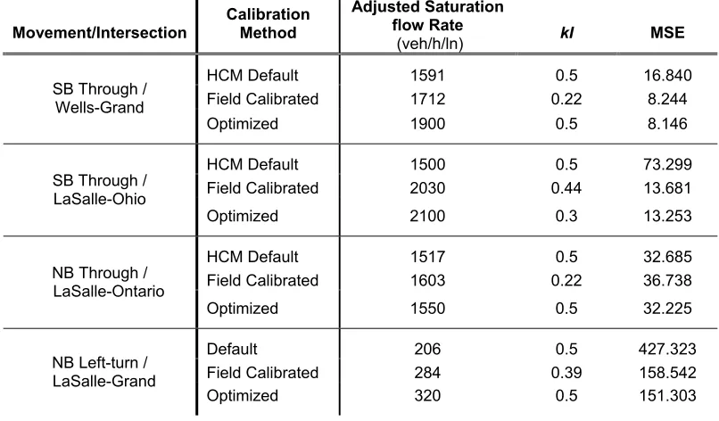
Table 4.1 Summary of Saturation Flow Rates, kI-values and Corresponding Control Delay MSEs by Different Methods

Movement/Intersection Calibration Method

Adjusted Saturation flow Rate

(veh/h/ln) kI MSE

HCM Default 1591 0.5 16.840

Field Calibrated 1712 0.22 8.244 SB Through /

Wells-Grand

Optimized 1900 0.5 8.146

HCM Default 1500 0.5 73.299

Field Calibrated 2030 0.44 13.681 SB Through /

LaSalle-Ohio

Optimized 2100 0.3 13.253

HCM Default 1517 0.5 32.685

Field Calibrated 1603 0.22 36.738 NB Through /

LaSalle-Ontario

Optimized 1550 0.5 32.225

Default 206 0.5 427.323

Field Calibrated 284 0.39 158.542 NB Left-turn /

LaSalle-Grand

Optimized 320 0.5 151.303

From Table 4.1, it can be seen that the saturation flow rate calculated using the HCM 2000 is

consistently the lowest when compared with the field calibrated and optimized values. For the

southbound through lane group at LaSalle-Ohio intersection, there is a significant difference

between the saturation flow rate calculated using the HCM equation with default values and that

obtained using field calibration or optimization. The calibrated and optimized saturation flow

rates even exceed the ideal saturation flow rate (1900 veh/h/ln) used in the HCM. However, for

northbound through lane group at Ontario-LaSalle intersection, the saturation flow rate estimated

using the three different methods are close, and the differences are less than 100 veh/h/ln.

(49)

38

calibrated values is quite close to that using the optimized values. However, in most cases, the MSEs are significantly high when the HCM default saturation flow rate and kI-value are used.

Only for the southbound through lane group at LaSalle-Ontario intersection, the control delay MSE based on the HCM default values is smaller than that based on field calibrated values. It is evident that the HCM control delay model may not accurately reflect the operation of studied lane groups when the HCM default values are used.

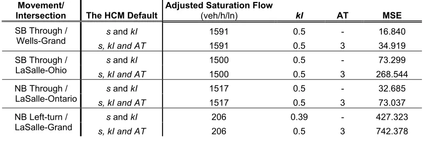
Usually, arrivals are assumed when estimating control delay using the HCM delay model, that is, Arrival Type 3 (AT3) is used. Table 4.2 shows the control delay MSE using the HCM default saturation flow rate and kI with/without default arrival type. For all studied lane groups, if the proportion of vehicles arriving on green is not considered cycle by cycle, the control delay MSE increases significantly. This indicates that the consideration of arrival type or proportion of vehicles arriving on green is necessary. The default arrival type may not appropriately reflect the real conditions of the studied lane groups. The analysis of the control delay using the HCM default saturation flow rate and kI-value for the individual lane groups in the following sections in this chapter is based on the incorporating cycle-by-cycle proportion of vehicles arriving on green.

The tuning parameters, saturation flow rate (s) and kI, may be not calibrated simultaneously. Table 4.3 shows the control delay MSEs with field calibrated saturation flow rate and/or kI. When only saturation flow rate is calibrated, the default value of kI = 0.5 is used, and when only