Approximate analysis of product-form type queueing networks with blocking and deadlock

(1)

Approximate Analysis of Product-Form Type

Queueing Networks with Blocking and Deadlock

by

H.G. Perros

A.A. Nilsson

and

Y.C.

Liu

Center for Communications and Signal Processing

Department of Electrical and Computer Engineering

North Carolina State University

December 1986

(2)

Approximate Analysis of Product-Form Type

Queueing Networks with Blocking and Deadlock

by

Harry G. Perros!

Department of Computer Science

and

A.A. Nilsson

Y.C. Liu

Department of Electrical

&

Computer Engineering

(3)

Abstract

(4)

Introduction

In recent years, there has been a growing interest in the development of

computa-tional methods for the analysis of queueing networks with blocking. This is

pri-marily due to a growing need to model actual systems which have finite capacity

resources, such as computer systems, telecommunication systems, distributed

sys-tems and flexible manufacturing syssys-tems.

In this paper, we consider queueing networks of the product-form type in which

some of the queues are finite. In particular, let us consider a class of closed

qltette-ing networks which is of the BCMP type, i.e., it satisfies local balance and has a

product-form solution.

In such queueing networks, each queue is assumed to be

infinite.

That is, it is large enough to accommodate all the units in the system. In

this paper, we consider such queueing networks, but we assume that some of the

queues have finite capacity. In view of this, the flow of units through one qlleue is

liable to getting blocked when a destination finite qllelle reaches its capacity

limita-tion.

The queues are assumed to be arbitrarily interconnected.

In view of this,

blocking of different nodes may cause deadlocks.

Deadlocks are assumed to be

detected and resolved instantaneously.

(5)

cer-routing matrix is reversible then the queueing network is also reversible and it has a

product-form solution (see Kelly[8] and Pittel[13]). This result holds under the

fol-lowing blocking mechanism. A unit at node

i

upon completion of its service chooses

destination node

j.

If node

j

is full at that moment, the unit starts a new service at

node i. Upon completion of its new service, the unit will choose a new destination

node independent of the destination node chosen the previous time. This is

repeated until the unit successfully enters a destination node. The same queueing

networks under the above mentioned blocking mechanism, also has a product-form

solution when the routing probability from nodes

i

to node

j

depends on tIle

number of jobs present at node i and

j

(see Kelly[8], Yao and Buzacott[16] and Le

Ny [9,10]). Other cases under which this particular queueing network has a

product-form solution have also been reported in the literature (see Hordijk and

Van Dijk[7] and Van Dijk[15]). Finally, Balsamo and Iazeolla[3] showed that in some

cases such a queueing network with blocking is equivalent to a queueing network

without blocking in terms of steady-state probabilities.

Other product-form solutions have been reported in the literature in connection

with two-node closed exponential queueing networks with finite queues. (see

Gor-don and Newell[6], Akyildiz[l], and Suri and Diehl[14]). A survey of these results

can be found in Perros[12].

(6)

a departure occurs from queue

j,

the ith server becomes unblocked and the unit

begins receiving service.

They obtained a product-form solution for this system

M

when the number of units N, is such that

N>

2:

111; -

N,

where

111;

is the maximum

;=1

capacity of queue

i,

i

=

I, 2, ... ,M.

They obtained this result using the notion of

"holes". Suri and Diehl[14] analyzed approximately the same tandem configuration

assuming that the first queue has a buffer

111}2':N.

Their analysis is based on a

decomposition method.

Yao and Buzacott[16] developed an approximation algorithm for analyzing arbitrary

configurations of closed queueing networks with blocking, assuming Coxian service

times and reversible routing. This algorithm is applicable to a closed queueing

net-work with blocking which has the following property. If the Coxian service

distribu-tions are substituted by exponential service distribudistribu-tions ( with the same mean),

then the resulting queueing network with blocking is reversible and has a

product-form solution.

Akyildiz[l] reported on an approximation algorithm for obtaining

the throughput and mean queue length of closed exponential queueing networks

with blocking assuming a blocking mechanism similar to the one considered in this

paper.

Finally, Onvural and Perros[ll] obtained analytical results that give some

insight into the structure of closed queueing networks with blocking.

(7)

network where each node is represented by either a finite or infinite queue. Each

queue (finite or infinite) is served by a single exponential server in a

FIFO

manner.

One class of unit is considered. Due to the finiteness of these queues blocking anti

deadlock can occur. TIle approximation algorithm uses a variant of Norton's

theorem.

Comparisons between approximate and exact results are given in section

4. Finally, conclusions are given in sections 5.

2.

Closed Exponential Queueing Networks with Blocking and Deadlock

Let us consider a closed queueing network consisting of M queues and N units.

Each queue i, i

=

I, 2.. M, is finite in size and is served by an exponential server

with mean service rate

J..Li.

Let

m,

be the maximum capacity of queue i, including

the one in service. We assume that the M queues are arbitrarily interconnected. A

unit at queue i, upon completion of its service choose to join node

j

with probability

1

1;i'

where

'LPi

j =

1. If queue

j

happens to be full at that particular instance, then

j

the unit will get blocked. That is, the unit is forced to wait in the ith server until it

succeeds in entering queue

j.

During this time the ith server is also blocked and it

can not serve any other units that might be waiting in its queue. The ith server

becomes unblocked the moment the blocked unit enters quelle

j.

Let us assume

now that there are several queues ( one of which is the above mentioned qtletle

i ),

all linked to queue

j.

Then it is possible that at any time there might be more than

one blocked unit waiting to enter quelle

j.

The maximum number of blocked units

will be equal to the number of its upstream quelles,

i.

e., queues directly linked to

queue

j.

It is assumed that these blocked units enter qlleue

j

on a

first-blocked-first-enter basis.

(8)

instance, assume that queue i is blocked by queue

j.

Now, it is possible that a unit

in queue

j

may, upon completion of its service, choose to go to queue i. If queue i

is full at that time, then deadlock will occur. It is assumed that deadlocks are

detected and resolved instantaneously. In this paper, it is assumed that a deadlock

is resolved by instantaneously exchanging blocking units. In general, this scheme

for

resolving

deadlocks

may

violate

the

first-blocked-first-enter

priority

rule

described above.

For instance, let us assume that queues i and k are blocked by

qtteue

j

in that order. That is, if a departure occurs from queue

j

the blocking unit

from queue i will enter queue

j

first.

Now, let us assume that the departing unit

from queue

j

chooses queue k as its destination, and, that queue k is full at that

moment.

This causes a deadlock to occur, which is resolved by simultaneously

exchanging the blocking units from queues

j

and k.

In view of this, the blocking

unit from queue k enters queue

j

first while queue i still remains blocked. Thus, the

first-blocked-first-enter priority rule has been violated.

We analyze this closed exponential queueing network with blocking and deadlock

numerically. This involved the following steps: (1) generation of all the states of the

system; (2) generation of the rate matrix Q; and (3) solution of the linear system

Qx

T

==

0 in order to obtain the steady state probability distribution.

2.1 Generation of the State Space

The state of the system under investigation is given by the vector

(111,112' · . · ,nM ),

where

11;

is the number of units in queue

i,

including the one in service. We have,

0<11;<111;.

Furthermore,

n, is allowed to assume the values 111;+1,111;+2, ... in order

to indicate which of the "upstream" queues are blocked and in what order.

(9)

three queues may be blocked at any time.)

M

Step 1: Generate a state such that

~ 1l;=N, 1l;$ln;.

That is a state in which no

;=1

blocking occurs. We refer to such a state as a

basic state.

Step

2:

For this basic state let

M'

be

the

set

of all

non-empty queues.

For

each

queue

i

E M',

let

M;'

be

the

set of all its downstream qllelles (directly linked to

queue i) which are at capacity. For each qllelle

j

EM/ generate a new state which

differs from the basic state by the fact that queue

i

is blocked by queue

j.

We call

such a state a

one-step blocking state, seeing that it involves blocking

of

one queue

only.

Step

3:

Given this one-step blocking state, generate a two-step blocking state

involv-ing one more blocked queue.

Step 4: From this two-step blocking state, generate a three-step blocking state.

Repeat until it is no longer feasible.

The nesting of these steps is as follows.

Generate a basic state until

*

begin

Generate a one-step blocking state until

*

begin

Generate a two-step blocking state until

*

begin

Generate a three-step blocking state until

*

end

end;

The symbol

*

is used to indicate the logical condition that state generation continues

until it is no longer feasible.

(10)

occurs each time the blocked queues form a cyclic directed graph. If deadlock has

occurred, then the deadlock resolution procedure described above is invoked in

order to determine the final state of the system.

The number of states associated with closed queueing networks with blocking

depends on the number of units in tile system, tile number of queues, the way

these qlleues are interconnected and the buffer capacities

of the qlleues. Figure I,

gives the number of states for

a

queueing network consisting of four fully connected

queues.

o

::

o

-..

. !

o a u

Nuaber of cue tOl'terc ,..

(11)

2.2 Generation of the rate matrix

Q

In order to generate the rate matrix by computer, we need to be able to associate an

integer with each state. This integer, referred to as the state number, is the ordinal

position of the state in the space as generated using tile algorithm described above.

TIle state number for a given state is obtained via a binary "dictionary" tree.

The

components of the state provide the keys which describe a path to the leaf which

contains the associated state number. Due to the frequency with which this routine

is called, it is perhaps the most time critical routine in the matrix generation

pr()-cedure.

TIle generation of the rate matrix, involves finding all the states which are accessible

from a state, as well as their corresponding transition probabilities.

A

state transition

occurs when a unit completes its service at a queue. Depending upon the current

state, the system may move to a state in which the unit has successfully entered its

destination queue, or to a state in which the unit is blocked. Blocking of this unit

mayor may not cause deadlock. If deadlock

OCC1lfS,

then the process moves with

zero transition time to a state obtained by allowing all the blocked units involved ill

the deadlock to instantaneously move to their respective destination queues.

2.3 Numerical Solution Technique

(12)

resulting vector has to be normalized to yield the stationary probability vector.

Experimental evidence showed that most of the CPU time was devoted to the

gen-eration of the state space and the rate matrix

Q.

TIle calculation of the stationary

probability vector required only a small fraction of the total CPU time.

Time

com-plexity problems emerged as the number of queues in the queueing network

increased and the interconnectivity of

these

qtteues became more complex.

As mentioned above, the non-zero elements of the rate matrix have no inherent

structure. We note, that we did not search for a possible enumeration of the state

space under which the rate matrix has a regular structure. The advantage of dealing

with

a matrix with a regular structure, is that one can avail of it in order to construct

an efficient algorithm for obtaining its stationary probability vector. However, such

an exercise was not necessary, seeing that the calculation of the stationary

probabil-ity was not

a

time-critical procedure.

Finally, we note that in this paper, we assumed that deadlock is detected and

resolved instantaneously.

However, this may not be the case in real-life systems.

In fact, it is more likely that detection and resolution may require an additional

delay. Such a delay can be easily incorporated in our model in view of the above

described numerical procedure.

3. The Approximate Procedure

In this section, we discuss an approximation procedure for analyzing closed

quetle-ing networks in which some of the queues are finite.

A

single class of customers

and exponentially distributed service times is assumed.

The approximation

pro-cedure is based on the well

knov

1

Norton's

theorem

(see

Chandy.

Herzog,

and

(13)

blocked into

a subnetwork hereafter referred to as the

blocking subnctuiork.

The

remaining infinite queues are grouped into a subnetwork that will be referred to as

the

non-blocking subnetuiork.

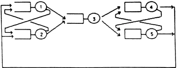
For example, consider a queueing network consisting of

five queues as shown in figure 2. Tile buffer sizes of queues 1,2 and 3 are assumed

to be infinite and the buffer sizes of queues 4 and 5 are finite. Due to the routing,

queue 4 may be blocked by queue 5 or vice versa. Also, queue 3 may be blocked by

queue 4 or queue 5. Hence, queues 3, 4 and 5 are grouped into the blocking

subnet-work, and queues 1 and 2 are grouped into the non-blocking subnetwork.

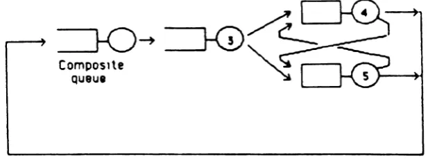
Fig. 2: A closed queueing network in which some of the queues are finite.

The approximation procedure can now be summarized as follows:

1.

Analyze the non-blocking subnetwork (obtained from the original network by

"shorting" the blocking subnetwork) as a product-form network assuming n

fixed units, where n= 1,2, ... ,N.

For each n obtain the steady-state

(14)

Sit is the set of all feasible states for given n. Based on these results calculate

the throughput T(n), n= 1,2, ... ,N.

2.

Construct a composite queue with a state-dependent throughput equal to

T(n), n= 1,2, ... ,N. Now, in the original network substitute the non-blocking

subnetwork by its equivalent composite qllelle. Analyze the reduced network

numerically using the algorithm described in section 2, to obtain the marginal

queue-length probability distribution for each queue, assuming N units in

it.

3.

Let

Pc

(11),

n= 1, ... ,N be the marginal queue-length probability that there are n

units in the composite queue as calculated in step 2. Then, from step 1 we

have

p(11)

=

J1(11

111)

_]1c(n ),

11

ES

_{n ,}

and n=1,2, ... ,N. Using

1

(11 )

the marginal

queue-length probability distribution for each queue in the non-blocking

sub-network can be easily obtained.

The marginal queue-length probability distribution obtained in steps 2 and 3

consti-tute an approximation to the true marginal queue-length probability distribution of

the original queueing network.

(15)

Fig. 3: Blocking subnetwork shorted

Composlte Queue

Fig. 4: Blocking subnetwork and composite queue

The above approximation algorithm also applies when the non-blocking subnetwork

is represented by any closed queueing network of the BeMP type.

(16)

4. Numerical Results

The above algorithm was implemented on an IBM

3081.

It

was employed to analyze

various configurations. The main result obtained is the queue-length distribution for

each node. From this, other more commonly sought performance measures, such as

throughput and mean quette length, can be easily obtained. The approximate

results were compared against exact numerical values. These exact numerical values

were obtained by analyzing the queueing network under study using the numerical

procedure described in section 2.

The results are summarized in tables 1 to 14. Each table gives the approximate and

exact results for the throughput, mean queue-length and queue-length distribution

per node. The relative error (expressed as a percentage) is also given.

The approximation algorithm gives, in general, good results.

The approximate

results for the throughput and mean queue length have a relative error less

than

1%.

Also, the approximate results for the queue-length distributions have a relative

error less than 5%.

(Some of the approximate queue-length probabilities have a

relative error as high as 60%. However, these cases are not significant seeing that

the probabilities are extremely small and they have an absolute error of less than

10-

6)

(17)

5. Conclusions

We developed a numerical procedure for analyzing closed queueing networks with

blocking and deadlock. This procedure was then used to develop an approximation

procedure based on Norton's theorem for analyzing queueing networks of the

product-form type in which some of the quelles have a finite capacity.

It was

shown through a number of examples that the approximation procedure is accurate

and tile relative error is small.

Tile numerical procedure was developed with a view to analyzing closed queueing

networks under a particular type of blocking.

It can be expanded, however. to

analyze such networks under different types of blocking mechanisms.

Also, it can

be easily extended to allow coxian distributed service times.

As was mentioned

ill

section 2, this procedure is not very efficient when analyzing large blocking

subnet-works. In this case, one can use the approximation method by Akyildiz[l], in order

to obtain the throughput of the blocking subnetwork. This procedure does not give

queue-length probability distributions. For tile special case where tile nodes are

indistinguishable, one can use an efficient numerical procedure given in Onvural

and Perros[ll].

The approximation procedure described in section 3 can be also applied in the

reverse way.

That is, we can first analyze the blocking subnetwork numerically

with a view to constructing an equivalent composite qlleue.

Then, replace the

blocking subnetwork in the original queueing network by its equivalent qllelte anti

analyze the resulting network as a product-form network.

This algorithm gives

similar results on those reported in tables 1 to 14.

(18)

blocking subnetwork can be replaced by an equivalent composite queue. The

result-ing network can then be analyzed as a product-form network. The feasibility of this

extension, however, needs to be investigated.

Acknowledgement

We would like to thank an anonymous referee for suggesting an improvement

011

(19)

References

1.

I. F. Akyildiz, "On the Exact and Approximate Analysis of Closed Queueing

Networks with Blocking,

'f

Computer Science Report 86-6, Univ. of Florida.

2.

T.

Altiok and H.G. Perros, "Approximation Analysis of Arbitrary

Configura-tions of Open Queueing Networks with Blocking", to appear in tile Annals of

Operations

Research,

3.

S. Balsamo and G. Iazeolla, "Some Equivalence Properties for

Queueing

Net-works With and Without Blocking,",

Periormance

'83,

Agrawala and Tripathi

(Eds.) Nortll-Holland (1983), 351-360.

4.

K.M. Chandy,

U.

Herzog, and L. Woo, "Parametric Analysis of Queuing

Net-works,"

IBM /. Res. Develop.

19, (1975) 36-42.

5.

K.M. Chandy, U. Herzog, and L. Woo, "Approximate Analysis of General

Queuing Networks,"

IBM

J.

Res.

Develop.

19, (1975) 43-49.

6.

W.].

Gordon and G.F. Newell, "Cyclic Queueing Systems with Restricted

Length Queues",

Operation Research

15 (1967), 266-278.

7.

A. Hordijk and N. Van Dijk, " Networks of

Queues

with Blocking",

Pcrior-mance'Bl ,

Kylstra (Ed.), Nortll-Hollanli (1981), 51-65.

8.

F.P. Kelly,

Reversibility and Stochastic Networks,

Wiley, New York, 1979.

9.

L.-M.

Le Ny,"Forme Produit

Pour

des Reseaux

Multiclasses

a

Routage

Dynamiques", Annales Scientifiques

de l'Universite de Clermont-Ferrand II,

76 (1983) 17-34.

10.

L.-M. Le

Ny,

"Etude Analytique de Reseaux de Files d' Attende Multiclass a

Routage Variable", RAIRO Recherche Operationnelle, 14 (1980), 331-347.

11.

R. Onvural, and H.G. Perros, "Some exact results for closed queueing

net-works with blocking," Computer Science report, N.

C.

State University, 1986.

(20)

13.

B. Pittel, "Closed Exponential Networks of Queues with Saturation: The

Jack-son Type Stationary Distribution and its Asymptotic Analysis,"

Math. of

Operation Research, Vol. 4, (1979), 367-378.

14.

R. Suri and G. W. Diehl, "A New Building Block for Performance Evaluation

of Queueing Networks with Finite Buffers,"

Proc. ACM SIGMETRICS

011

Mcns-urement and

Modelil1g of

Computer

SyStC111S,

Cambridge, Mass., (1984) 134-142.

Conference Proceedings, Cambridge, Mass.,(1984) 134-142.

15.

N. Van Dijk, "Controlled Markov Processes: Time Discretization-networks of

Queues", Ph.D. thesis Mathematical Centrum, Amsterdam (1983).

(21)

Table 1: The configuration analyzed is shown in Figure 2. m₁

=

m₂ = mJ = 00 , m4

=

2, ms = 3 ; JLl

=

fL3

=

f.14= 0.5 , ~2 = ~S = 1; P12 = 0.7, PI3 = 0.3, P21

=

0.5, P23

==

0.5. P34 = 0 ..1. P35

==

0 ..), P41

=

0.5. P42

=

0.25. P45

=

0.25,

PSI = 0.25, PS2 = 0..1. P54 = 0.25: :'.j

==

6. Throughput node 1 node 2 node 3 node 4 node 5

Mean queue length node 1 node 2 node 3 node 4 node 5 Exact Solution 4.055e-Ol 4.,)96e-01 :3.,) 14e-O 1

~.3"'3e-n1 2.343e-O1 Exact Solution 2.312e+OO 7.770e-Ol 1.916e+OO 6.68ge-O1 3.270e-Ol Approximation 4.047e-Ol -t.·587 e-O 1 1..j16e-O 1

~. ~44e-O1

:!.344e-O 1

.-\pproximation 2.310e+OO 7.743e-Ol 1.91ge+OO 6.694e-OI 3.274e-Ol Error(%) 2.0e-Ol 2.0e-Ol 5.7e-O~ 4.3e-02 4.3e-02 Error(~) 8.7 e-02 3.5e-Ol l.6e-Ol 7.5e-02 1.2e-Ol

Queue Length Distribution at Node 1

Number of units Exact Solution

o

1.890e-Ol 1 I.900e-Ol 2 1.840e-Ol 3 1.673e-Ol 4 1.372e-Ol 5 9.248e-02 6 4.008e-02

(22)

o

2.396e-Ol

1 2.214e-OI

2 1.962e-Ol

3 1.606e-OI

4 1.098e-O1

5 5.33ge-02

6 1.894e-O~

);urnber of units Exact Solution

o

.5.30ge-Ol

1 2.693e-Ol

2 1.998e-Ol

o

7.470e-Ol

1 1.923e-Ol

2 4.761e-02

3 1.316e-02

Approximation 2.390e-Ol 2.213e-Ol 1.961e-O 1 1.606e-Ol 1.103e-O 1 :>.354e-02

1.914e-02

Approxi mation ;J.307 e-O 1 2.693e-Ol 2.001e-Ol

Approximation 7.468e-Ol

1.923e-Ol

4.767e-02

1.323e-02

Error(%) 2.5e-O I 4.5e-02

5.1e-02

O.Oe+OO 4.6e-Ol 2.8e-Ol 1.1e+OO

Error(

ce)

3.8e-02 O.Oe+OO

1.5e-O!

(23)

Table 2: The configuration analyzed is shown in Figure 2. m_l = m2 = mJ = 00 ,

m₄

=

2, m s= 3 ; f.LI

=

f.LJ

=

JL4

=

0.5 , f.L2 = f.Ls = 1 ; Pl2 = 0.7, PI3 = 0.3, P21 = 0.5~ P23 = 0.5, P34

=

0.5, P3S = 0.5. P41 = 0.5. P42

=

0.25. P4S = 0.25. PSI

=

0.25, PS2

=

0.,5.PS4 = 0.25; N = 15.

Throughput Exact Solution Approximation Error(%)

node 1 4.696e-O1 4.69Se-Ol 4.3e-02

node 2 5.322e-O1 5.325e-0 1 ,j.6e-02

node 3 -t'()71e-O1 4.07~e-O1 2.5e-02

node 4 2.714e-Ol 2.715e-O 1 3. '7 e-02

node 5 2.714e-O1 2.715e-OJ 3. '7 e-02

Mean queue length Exact Sol ution .Approximation Error(%)

node 1 6.'798e+OO 6.815e+OO 2.5e-Ol

node 2 1.113e+OO 1.115e+OO 1.8e-O!

node 3 5.853e+OO 5.833e+OO 3.4e-Ol

node 4 8.161e-Ol 8.165e-Ol 4.ge-02

node 5 4.200e-Ol 4.203e-Ol 7.1e-02

Number of units Exact Solution Approximation Error(%)

0 6.08ge-02 6.035e-02 8.

s-.or

1 6.440e-02 6.354e-02 1.3e+OO

2 6.746e-02 6.671e-02 1.le+OO

3 6.973e-02 6.933e-02 5.7e-Ol

4 7.136e-02 7.132e-02 5.6e-02

5 7.260e-02 7.284e-02 3.3e-Ol

6 7.355e-02 7.395e-02 5.4e-Ol

7 7.416e-02 7.463e-02 6.3e-Ol

8 7.428e-02 7.474e-02 6.2e-Ol

9 7.362e-02 7.402e-02 5.4e-Ol

10 7.170e-02 7.201e-02 4.3e-Ol

11 6.779e-02 6.801e-02 3.2e-Ol

12 6.088e-02 6.099e-02 1.8e-Ol

13 4.967e-02 4.972e-02 1.0e-Ot

14 3.343e-02 3.340e-02 9.0e-02

(24)

Number of units _{Exact Solution}

Approximation _Error(%)

0 _4._{678e-O 1}

4.67 5e-O 1 _6.4e-02

1 _{2.511e-O 1}

2.511e-O1 _O.Oe+OO

C)

1.341e-O 1 _1.340e-Ol _'7.5e-02

..

3 _7.102e-02

7.097 e-02 _7.0e-02

4 _3.722e-02

3.724e-02 _5.4e-02

5 _1.928e-02 _1.935e-02

3.6e-Ol

6 _9.870e-03

9.93ge-03 _'7_.Oe-OI

-

• 4.9S1e-03 _,1.038e-03 _1.1e+OO

8 _2.4'71e-03

2.512e-03 _1.7e+OO

9 _1.201e-03 _1.2~6e-03

2.1e+OO

10 _·j.670e-04 _,1.813e-04

~.,)e+OO

11 _~.574e-04 _~.6-t7e-04

~.8e+OO

12 _l.100e-04 _1.133e-04

3.0e+OO

13 _4.251e-05 _4.381e-05

3.1e+OO

14 1.35.5e-05 _1.398e-05 _3.2e+OO

15 2.797e-06 _2.886e-06 _3.2e+OO

Number of units Exact Solution _{Approximation} _Error(%)

0 8.957e-02 8.908e-02 5.5e-Ol

1 8.594e-02 8.586e-02 9.3e-02

2

8.294e-02 _8.323e-02 _3.5e-Ol

3 8.04ge-02 8.103e-02 6.7 e-Ol

4 7.844e-02 7.909e-02 8.3e-Ol

5 7.661e-02 7.728e-02 8.7e-Ol

6 7.485e-02 7.545e-02 8.0e-Ol

7 7.300e-02 7.347e.02 6.4e-Ol

8 7.084e-02 7.114e-02 4.2e-Ol

9 6.806e-02 6.8l2e-02 8.8e-02

10 6.394e-02 6.371e-02 3.6e-Ol

11 5.701e-02 5.647e-02 9.5e-Ol

12 4.665e-02 4.589e-02 1.6e+OO

13 3.14ge-02 3.073e-02 2.4e+OO

14 1.490e-02 1.437e-02 3.6e+OO

(25)

o

4.55ge-OI

1 2.721e-OI

2 2.720e-Ol

Queue Length Diecribution at Node 5

o

6. 971e-O1

1 2. 118e-O 1

2 6.~03e-02

3 2.60~e-02

Approxi mation 4.557e-OI 2.721e-0 1 2.722e-0 1

Approxi mat ion 6.970e-O1 2.118e-Ol

6.5082-02

~.60ge-O~

Error(%) 4.4e-02 O.Oe+OO 7.4e-02

Error(O"f) 1.4e-02

O.Oe~OO

(26)

Table

3: The configuration analyzed is shown in Figure

2.

m

t

=

m2= m3

=

ooI

m.

=

1, IDS

=

2 j

~l

=

~3

=

~4

=

0.5 I

~2

=

~5

=

1 ; P12

=

0.7, P13

=

0.3.

P21

=

0.5, P23

=

0.5. P34

=

0.5, P35

=

0.5. P41

=

0.5. P42

=

0.25, P45

=

0.25. PSI

=

0.25, PS2 = 0 ..5. Pc;.

=

0.25; ~

=

1.5.

Throughput _{Exact Solution}

Approximation _Error(%)

node 1 _4.433e-Ol

4.434e-Ol 2.3e-02

node 2 _5.023e-Ol

5.026e-O 1 _6.0e-02

node 3 _{3.83ge-O 1} _{3.843e-O 1}

1.Oe-O 1

node 4 _{:!.5.5ge-O 1} _2.562e-Ol

1.2e-O1

node 5 _{2.5.5ge-O 1} _2.56~e-O₁

1.2e-O1

~ean queue length _{Exact Solution} _{Approximation}

Error(%)

node 1 _5.102e+OO _5.084e+OO

3.5e-Ol

node 2 _9.845e-Ol _9.880e-Ol

3.6e-Ol

node 3 _7.988e+OO _8.00te+OO

1.6e-Ol

node 4 _5.154e-Ol _5.15ge-Ol

9.7e-02

node 5 _4.100e-OI _4.106e-Ol

1.5e-Ot

Number of units Exact Solution Approximation _Error(%)

0 1.133e-Ol 1.13te-OI I.Se-OI

I 1.IOIe-Ot 1.093e-Ol 7.3e-Ol

2 1.03ge-Ol _1.038e-Ol _9.6e-02

3

9.554e-02 9.62Ie-02 7.0e-01

4 8.690e-02 8.791e-02 1.2e+OO

5 7.868e-02 7.967e-02 1.3e+OO

6 7.107e-02 7.186e-02 1.1e+OO

7 6.406e-02 6.457e-02 S.Oe-OI

8 5.756e-02 5.778e-02 3.8e-Ol

9 5. 144e-02 5.137e-02 l.4e-OI

10 4.550e-02 4.517e-02 7.3e-Ol

II 3.946e-02 3.89le-02 1.4e+OO

12 3.295e-02 3.228e-02 2.0e+OO

13 2.550e-02 2.483e-02 2.6e+OO

14 1.676e-02 1.624e-02 3.1e+OO

(27)

Number of units _{Exact Solution} _{Approximation} _Error(%)

0 4.977e-Ol 4.97 4e-O1 6.0e-02

1 2.530e-Ol 2.52ge-O 1 4.0e-02

2 1.27 3e-O1 1.271e-O 1 1.6e-Ot

3 6.307e-02 6.305e-02 3.2e-02

4 :3.081e-02 3.094e-02 4.2e-O 1

5 1.486e-02 1.504e-02 1.2e+OO

6 7.080e-O:3 ; .231e-03 2.1e+OO

7 3.331e-03 3.436e-03 3.2e+OO

8 1.543e-03 i.60ge-03 4.3e+OO

9 7.018e-04 7.388e-04 5.3e+OO

10 3.112e-04 3.307e-04 6.3e+OO

11 1.333e-04 1.427 e-04 7.1e+OO

12 5.410e-05 5.823e-05 7.6e+OO

13 2.010e-05 2.168e-05 7.ge+OO

14 6.300e-06 6.782e-06 7.7e+OO

15

1.286e-06 1.383e-06 7.5e+OO

Number of units Exact Solution Approximarion Error(%)

0 3.701e-02 3.580e-02 3.3e+OO

1 4.04ge-02 3.955e-02 2.3e+OO

2

4.42ge-02 4.36ge-02 1.4e+OO

3 4.865e-02 4.835e-02 6.2e-Ol

4 5.358e-02 5.357e-02 I.ge-02

5 5.910e-02 5.936e-02 4.4e-OI

6 6.5I9e-02 6.570e-02 _7.8e-OI

7 7.180e-02 7.253e-02 _1.0e+OO

8 7.878e-02 7.969e-02 1.2e+OO

9 8.580e-02 8.677e-02 1.1e+OO

10 9.207e-02 9.294e-02 _9.4e-Ol

11 9.596e-02 9.650e-02 _5.6e-Ol

12 9.345e-02 9.338e-02 _7.5e-02

13 7.621e-02 7.555e-02 _8.7e-Ol

14 4.57ge-02 _4.511e-02 _1.5e+OO

(28)

Queue Length Distribution at Node4

o

4.846e-Ol

1 5.154e-Ol

o

6.850e-Ol

1 2.201e-Ol

2 9.494e-02

Approxi mation 4.841e-Ol 5.15ge-O1

Approximation 6.846e-Ol 2.202e-Ol 9.516e-02

Error(%)

I.Oe-Ot

9.7e-02

(29)

Table 4: m_t = m2

=

m₃ = "X) , m₄= 2; ....1= 1, ....2

=

0.5, ....3 = 1,fJ.. = 0.5; and

N

=

6.

Throughput Exact Solution Approximation Error(%)

node 1 4.007e-Ol 4.002e-Ol 1.2e-O 1

node 2 4.007e-Ol 4.002e-Ol 1.2e-Ol

node 3 4.007e-Ol 4.003e-Ol 1.0e-Ol

node 4 4.007e-Ol 4.003e-Ol I.Oe-Ol

~ean queue length Exact Solution Approximation Error(%)

node 1 6.205e-Ol 6.281e-Ol 1.2e+OO

node 2 2.302e+OO 2.295e+OO 3.0e-Ot

node 3 1.691e+OO 1.692e+OO 5.ge-02

node 4 1.387e+OO 1.385e+OO 1.4e-Ol

Number of units ExactSolution Approximation Error(%)

0 5.993e-Ol 5.998e-Ol 8.3e-02

1 2.505e-OI 2.480e-Ol I.Oe+OO

2 9.938e-02 9.846e-02 9.3e-Ol

3 3.599e-02 3.682e-02 2.3e+OO

4 1.121e-02 1.255e-02 1.2e+Ol

5 3.005e-03 3.636e-03 2.le+Ol

6 5.655e-04 7.195e-04 2.7e+Ol

Number of units Exact Solution ..\ pproxi mation _Error(~)

0 1.986e-Ol 1.996e-O 1 5.0e-O 1

1 1.91 :?e-O 1 1.9 17e-O1 2.6e-Ol

2 1.-g8r-Ol 1.78ge-O 1 1.6p-O:;

3

1..j94e-O 1 1.~9~e-O1 6.3e-02

4 1.315e-O 1 1.11~p-nl _~.3e-O 1

5 9.39~~-O~ Q . :r3:2p - ()~ _6.7e-O}

(30)

o

2.650e-Ol

1 2.228e-Ol

2 2.034e-Ol

3 1.832e-O 1

4 1.17ge-O1

5 6.491e-03

6 1.197e-03

Queue Length Distribution at ~ode 4

~urnber of units Exact Solution

o

1.

sss-.o:

1 2.158e-Ol

2 5.856e-Ol

Approximation 2.665e-Ol 2.230e-0 1 2.021e-O 1 1.794e-O 1 1.196e-Ol 7.878e-03 1.466e-03

Approximation I.

sss-.o:

2.162e-Ol 5.843e-Ol

Error(%) 5.7e-Ol 9.0e-02 6.4e-Ol 2.1e+OO

1.4e+OO 2.1e+Ol 2.2e+OI

(31)

Table 5:

m,

=

'"2

=

m₃

=

'XJ, m₄

=

5; ~1 1, ... ,

=

0.5, ....3

=

1, ...4

=

0.5; and N 15.

Throughput Exact Solution Approximation Error(o/n)

node 1 4.635e-Dl 4.635e-Ol O.Oe+OO

node 2 4.635e-ol 4.635e-Ol O.Oe+OO

node 3 4.635e-Gl 4.635e-Ol O.Oe+OO

node 4 4.635e-Dl 4.635e-Ol O.Oe+OO

Mean queue length Exact Solution Approxima tion Error(% )

node 1 8.490e-Ol 8.541e-Ol 6.0e-Ol

node 2 6.563e- 00 6.571e+ 00 1.2e-Ol

node 3 3.838e-OO 3.840e+OO 5.2e-02

node 4 3.742e~00 3.743e+ 00 2.7e-02

Number of units Exact Solution Approxima tion Error(Cj(l )

0 5.365e-Ql 5.365e-Ql O.Oe+OO

1 2.505e-ol 2.500e-Ql 2.0e-Ol

2 1.162e-Ql 1.158e-Ol 3.4e-Ol

3 5.345e-D2 5.336e-02 1.7e-Ol

4 2.427e-D2 :!.440e-02 5.4e-Ol

5 1.083e-D2 1.106e-02 2.1e+ 00

6 4. 722e-03 4.961e-03 S.le-4-00

7 2.00ge-03 2.:!OOe-03 9.5e-+- 00

8 8. 360e-04 9.600e-04 1.5e-;(l1

9 3.404e-04 4.106e-04 2.1e-'-Ol

10 1.351e-04 1.710e-04 2.7e+Ol

11 5.185e-03 6.858e-05 3.2e+ 01

12 1.8q2e-tJ~

2.

~n2e-n:; ~.Re+01

13 6.354e-tlh q.1121e-llh -±.2e-L(11

14 1.825e-()h _2.h~4e-Oh _.f._3e-r-01

(32)

Queue Length Distribution at Node 2 Number of units

o

1 2

3

4 5 6 7 8 9 10 11

12

13 14

15

Exact Solution 7. 296e-02 7.2QOe-02 7.27ge-02 7.260e-02 7.232e-02 7.1Qle-02 7.136e-02 7.061 e-(l:! 6. QSRe-02 6 811e-02 6.586e-02 6.232e-02 5.668e-02 4.786e-02 3.4ne-02 1.737e-02

A pproxima tion

7.310e-02 7.J02e-02 7.2QOe-02 7.271e-02 7.242e-02 7.201e-02 7. 144e-02 7.066e-02 6.95Qe-02 6.807e-02 6.577e-02 6.218e-02 5.651e-02 4.76ge-02 3.463e-02 1.730e-02 Error(o/n) 1.ge-Ol 1.he-Ol 1.Se-Ol

i.s--oi

l.-ie-Ol 1.4e-Ol 1.1e-Ol 7.1 e-02 1.4e-02 5.ge-02 1.4e-Ol 2.2e-01 3.0e-Ol 3.6e-Ol 4.0e-01 4.0e-Ol

Queue Length

Distribution at

Node 3

Number of units

o

1 2

3

4 5 6 7 8 9 10 11 12 13 14 15 Exact Solution 2.003e-Ql 1.323e-ol 1.003e-01 8. 536e-02 7. 858e-02 7.556e-02 7.415e-D2 7.308e-D2 7.102e-D2 6.504e-D2 4. 15ge-D2 1.980e-D3 5. 347e-D4 1.479e-04 3.78Se-oS 7.057e-D6

A pproxima tion

2.003e-Ol 1.324e-Ol 1.003e-Ol 8. 544e-Q2 7.86ge-Q2 7.56ge-Q2 7.425e-Q2 7. 29ge-02 7.044e-02 6.34ge-02 4.226e-02 2.730e-D3 7.756e-04 2.224e-Q4 5.850e-05 1.111e-05 Error(% ) O.Oe+ 00 7.6e-02 O.Oe+OO 9.4e-02 1.4e-01 I.7e-01 1.3e-Ol 1.2e-Ol 8.2e-Ol 2.4e+ 00 1.6e+OO 3.8e+01 4.5e4-01 5.0e+ 01 S.Se+01

S.7e-Ol

Queue Length Distribution at Node ~

o

7.305e-D2

1 7.686e-O~

2 8.448e-02

3 Q.gQ3e-02

4 1.317e-111

Approximation 7.301e-O~ -;.hR3e-0:2 8.-!4he-02 t) QC)~tl-n2 1.31:-e-Ol

Errortti;" ) ~.5e-02

3.Qe-02 2.4e-n2

u.Pe-

no

ll.ne---

no

(33)

Table 6: m₁

=

m_{2 =} m₃

=

m_{4 =} m, -== IX) , m

h == 2, m7 = 3; ~1 == .... ::; = 1.0, ~2

=

JL3 = ~4 =:

~6

=

~7

=

0.5; P12 == 0~5, P13 == 0~25, P14

=

~.25, P25

=

_1.0, P35

=

1.0,P45

=

1.0, P56 =

0.5, PC;i = 0.5, PhI

=

O..J, Ph7 == O.J, Pil

=

0.o. P7h

=

0.o: N == 6

Throughput Exact Solu tion Approximation Error(9o )

node 1 3.542e-Ol 3. 543e-Ql 2.8e-02

node 2 1.770e-Ql 1.77Ie-Ol 5.6e-02

node 3 8.855e-Q2 8.857e-02 2.3e-Q2

node 4 8.855e-D2 8.857e-Q2 2.3e-D2

node 5 3.541e-Dl 3.542e-Ol 2.8e-02

node 6 3.542e-ol 3. 542e-Dl O.Oe+ 00

node 7 3.542e-Ol 3.542e-Ol O.Oe+OO

node 1 5.334e-ol 5.302e-Dl 6.0e-Ql

node 2 5.301e-Dl 5.302e-Ql 1.ge-02

node 3 2.136e-ol 2. 136e-Dl O.De-+-00

node 4 2. 136e-Ql 2. 136e-Ql O.Oe..;..OO

node 5 1.208e~00 1.20ge-- 00 _8.3e-02

node 6 1.35ge-- 00 _1.360e-OO _7.4e-02

node 7 1.942e-.r 00 _{1.943e- 00} _5.1e-D2

Number of units Exact Solu hon _{Approximation} _Error(_{Dr )}

0 6.458e-Ol _6._-t_57'_e_-01 _1.5e-fl2

1 2.291e-Ol _2.312e-Ol _Q.2e-Ol

2 8.466e-02 _R.356e-02 _{1.3e- 00}

3 2.Q28e-02 _~.₈_~qe-tl:: _{2.-le - 00}

4 8.77ge-03 _S.5b2e-Ll~ _{2.5e - 00}

5 ~.05ge-03 _2.n1~e-{1~ _{2.3e -}

'on

(34)

o

6.45ge-Ol

1 2.310e-Ol

2 8.36ge-D2

3

2.85ge-U2

4 8.553e-03

5 2.011e-03

6 2.86ge-04

Approximation 6.457e-Ol

2.312e-Ol 8.356e-02 2.85ge-02 8.561e-03 2.012e-03 2.865e-04

Errort's-)

3.1e-02

8.7e-02

1.6e-Ol

O.Oe-+-OO 9.4e-02

j.Oe-U2

(35)

Number

of units Exact Solution Approximation Error(% )

0 8.22ge-Ol 8.22ge-Ol O.Oe+OO

1 1.-l62e-Ol 1.-!64e-Ol l.~e-Ol

2 2.590e-02 2.582e-O~ 3.1e-Ul

3 4.265e-03 4.253e-03 2.Re-Ol

4 6.088e-04 6.070e-04 3.0e-Ol

5 6.767e-OS 6.735e-05 4.7e-Ol

6 4.50ge-06 4.4:77e-06 7.1e-Ol

Number of units Exact Solu tion _{Approxima tion} _Error(CJr )

0 8.22ge-Ol 8.22ge-Ol O.Oe~00

1 1.-l62e-Ol 1.464e-Ol 1.4e-Ol

2 2.590e-02 2.582e-02 3.1e-O!

3 4.265e-03 4.253e-03 2.8e-01

4 _6.088e-04 _6.070e-04 _3.0e-Ol

5 6.767e-DS 6.735e-QS 4.7e-Ol

6 4.50ge-06 4.477e-Q6 7.1e-Ol

Number of units Exact Solution Approxirna tion Error(% )

0 2.914e-Ol 2.924e-ol 3.4e-Ol

1 _3.667e-Ql _3.651e-Dl _4.4e-Ol

2 2.151e-Ql 2.150e-Dl 4.6e-02

3 9.932e-02 _9.946e-ol _1.4e-Ol

4 _{2. 472e-02} _{2. 520e-D2} _1.ge+OO

5 2.420e-Q3 2.575e-Q3 6.4e+OO

6 3. 367e-Q4 _3.562e-D4 _5.8e+OO

Number of units Exact Solu Han _Approxima_tion _Error(9n)

0 1.953e-Ol 1.950e-DI _I.Se-Ol

1 2.502e-Ol _2.502e-Ol _O.Oe+OO

2 5.545e-Dl _5.548e-DI _S.4e-02

Number of units _{Exact Solu tion} _{Approximation} _Error(_(/~₎

0 1.442e-Ol _1.43Qe-Ol _2.1e-Ol

1 1.98ge-Ol _1.QS7e-nl _1.Oe-Ol

2

2.:274e-O1 _2.2:-5e-nl _4.4e-(12

(36)

Table 7: m_t

=

m₂

=

m

=

m

=

m

=

'X) m - 2 m - 3'" - 1 U

-3 4 5 ' " - , 7 - 'r-l - ~j = ., ~2 - ~3

=

~4

=

~6..

=

~7

_=

0.5; PI:! ~ 0__5, Pu

=

0__25, PI4

=

~.25, P:!~

=

1.0, P3~

=

1.0,P4~

=

1.0, P"f,

=

O.,J, F5i - 0.5, Phi - 0.:'1, Pni ~ O.J, F71 ~ 0.o, Pin

=

0.5; N

=

8

Throughput Exact Solu tion A pproxima tion Error(9'1')

node 1 3.62ge-Ol 3.62ge-ol O.Oe+OO

node 2 1.814e-Ql 1.814e-Ql O.Oe+OO

node 3 9.071e-Q2 9.072e-Q2 1.1e-02

node 4 9.071e-Q2 9.072e-02 1.1e-02

node 5 3.62ge-Ql 3.62ge-ol O.Oe+OO

node 6 3.62ge-Ql 3.62ge-Ql O.Oe+ 00

node 7 3.62ge-Ql 3.62ge-Ql O.Oe+OO

Mean queue length Exact Solution Approximation Error(o/(l )

node 1 5.755e-Ql 5.694e-Ql 1.]e+OO

node 2 5.698e-Ql 5.694e-Ql 7.0e-02

node 3 2.224e-Dl 2.223e-ol 4.5e-02

node 4 2. 224e-Ql 2.223e-Ql 4.5e-02

node 5 2.595e+ 00 2.603e+ 00 3.1e-Ol

node 6 1.540e-t-OO 1.S40e+ 00 O.Oe+OO

node 7 2.274e~00 2.274e+OO O.Oe+ 00

Number of units Exact Solution A pproxirnation Error(CJ(' )

0

6.371e-Ol 6.371e-Dl O.Oe-+- 00

1 2.254e-Ol 2.2RQe-Ol 1.6e~()O

2 8.694e-D2 8.532e-(l2 1.qe -

no

3 3.310e-D2 3.178e-02 4.0e-i-00

4 1.196e-02 1.14qe-(l2 3.Qe-

on

5 3.990e-03 3.Rfi8e-l1~ 2.6e-l1O

6

1.166e-03 1. 1~3t"\-(1~ 1.1

e

-l1(l

7 2.688e-l).J ~ h")l ..,-11..1 1. 1e-tl )

(37)

Number of units Exact Solu tion Approximation Error(o/fl )

0 6.372e-ol 6.37le-ol 1.6e-02

1 2.286e-Ol 2.28ge-Ol 1.3e-Ol

.,

8.561e-02 8.532e-02 3.4e-Ol

...

3 3.182e-02 3.I78e-02 1.3e-Ol

4 1.148e-02 1.I4Qe-02 8.7e-02

5 3.894e-03 3.887e-03 I.8e-Ol

6 1.161 e-03 1.153e-03 6.ge-O1

-

I 2.72Re-04 2.69(1e-()4 1.~e.J-

no

8 3.894e-05 3.817e-OS 2.0e--OO

Number of units Exact Sol u tion A pproximation Errorr'z-)

0 8.186e-Ql 8.186e-Ol O.Oe+OO

1 1.478e-Ol 1.480e-Ol 1.4e-Ol

2 2.756e-02 2.741e-02 5.4e-Ol

3 5.0S0e-Q3 S.02Se-03 S.Oe-01

4 8.885e-04 8.855e-Q4 3.4e-Ol

5 1.452e-04 1.443e-04 6.2e-Ql

6

2.064e-QS 2.042e-oS 1.1e+OO

7 _2.292e-06 _{2. 252e-06} _1.7e+OO

8 1.527e-Q7 1.492e-07 2.3e+OO

Number of units Exact Solution _{Approximation} _{Error(% )}

0 8. 186e-Ql

8.

isee-or

_O.Oe+OO

1 1.478e-Ql 1.480e-Ql 1.4e-Ql

2 2.756e-Q2 _2.741e-Q2 _S.4e-ol

3 5.050e-03 _5.025e-03 _S.Oe-Ol

4 8.88Se-Q4 8.855e-Q4 _3.4e-Ol

5 1.452e-Q4 _1.443e-04 _6.2e-Ol

6 2.064e-05 2.042e-QS _1.1e+OO

7 2.292e-06 _2.252e-D6 _{1.7e-r- 00}

(38)

Number

of units

Exact Solution

o

6.917e-02

1 1.32ge-OI

2 2.467e-Ol

3 3.258e-OI

4 I.SOle-Ol

5 6.135e-02

6 1.298e-02

7 8.15ge-04

8 1.072e-04

o

1.288e~1

1 2.022e-Ol

2 6.691e-Ol

o

8.552e-02

1 1.384e-Ql

2 1.926e-Ol

3 5.835e-Ql

Approximation

7.008e-02 1.34Ie-Ol

2.438e-OI 3.214e-Ol I.525e-OI 6.317e-02 1.387e-02 9.982e-04 1.311e-04

Approximation

1.288e-Ol 2.023e-Ol 6.68ge-Ql

Approximation

8.554e-Q2 1.385e-ol 1.928e-Ol 5.832e-ol

Error(% ) 1.3e+OO 9.0e-Ol

1.2e+ 00 1.4e+OO

1.6e+OO

3.0e+ 00

6.ge-+- 00

2.2e+01 2.2e+ 01

Error(~7())

O.Oe+ 00 4.ge-02 3.0e-02

(39)

Table 8: m

1 == m2

=

m3

=

m4

=

00, mS

=

3; ~l == ~3 :: ~4

=

0.5, J.l2

=

~~ = 1.0; P12 == 0.7,

P13 = 0.3, P21

=

0.5, P24

=

0.5, P31

=

0.25, P32

=

0.25, P35

=

0.5, P~1

=

0.25, P42 = 0.25,

PolS == 0.5, p)}

=

0.5, P52

=

0.5; N

=

6

node 1 4.64ge-Ol 4.64ge-Ql O.Oe+OO

node 2 5.26ge-Ol 5. 26ge-()1 O.Oe+OO

node 3 1.395e-tll 1.395e-ol O.Oe+OO

node 4 2.635e-QI 2.635e-Ol O.Oe+OO

node 5 2.015e-Ol 2.015e-ol O.Oe+OO

Mean queue length Exact Solution Approximation Error(o/n)

node 1 3.387e+ 00 3.386e+ 00 3.0e-02

node 2 9.934e-Ql 9.933e-ol 1.0e-02

node 3 3.me-Ol 3. 778e-ol 2.6e-02

node 4 9.94ge-Dl 9.951e-Ql 2.0e-02

node 5

2.473e-Ol 2.473e-01

O.Oe+OO

Number of units Exact Solution Approximation Error(7(l )

0 7.01ge-Q2 7.023e-02 5.7e-02

1 1.OOge-Ql I.OIOe-Ol 9.ge-02

2 1.386e-Ql 1.386e-Ol O.Oe+ 00

3 l.me-Ol 1.777e-Ol O.Oe~OO

4 2.03ge-OI 2.03ge-01 O.Oe~O(1

5 1.922e-OI 1.922e-Ol

u

Oe+

no

(40)

Number of units

o

1 2

3

4 5 6

Exact Solu tion

4.731e-Ol 2.607e-Ul 1.406e-Ol 7.275e-02 3.482e-D2 1.418e-02 3.856e-03 Approximation 4.731e-tll 2.607e-Ol 1.40Se-Ol 7.275e-Q2 3.482e-02 1.418e-02 3.856e-03 Error(o/n) O.Oe+OO O.Oe-t-.OO 7.1e-02 O.Oe+OO O.Oe+OO O.Oe+ 00

O.Oe-4-00

o

7.207e-Ol 1 2.046e-Ol 2 5.606e-Q2 3 1.450e-D2 4 3.403e-03

5

6.653e~ 6 8.493e-05

o

4.724e-Ql 1 2.610e-Ol

2

1.40ge-Ol 3 7.290e-02 4 3.485e-Q2 5 1.41ge-Q2

6

3.861e-Q3

o

7.985e-Dl 1 1.626e-Ol 2 3.191e-02 3 6.96ge-03 Approximation 7.206e-Ol 2.046e-Ol 5.608e-02 1.451e-02 3.405e-03 6.663e-04 8.S14e-oS

A

pprox ima

tion

4.723e-Ol 2.610e-Ql 1.40ge-ol 7.291e-D2 3.485e-02 1.421e-02 3.868e-03 Approximation 7.98Se-Dl 1.626e-ol 3.192e-02 6.974e-03

Error(C;" ) 1.4e-02 O.Ge-+00

(41)

Table 9: m_I

=

m₂

=

m₃

=

m₄

=

00, m

5

=

3; f-ll = f-l3

= ....

4

=

0.5, f-l2 - ....5

=

1.0; P12

=

0.7, PI3

=

0.3, P2I

=

0.5, P24

=

0.5, P31

=

0.25, P32 == 0.25, P35 == 0.5, P41

=

0.25, P42

=

0.25,

P

45

=

0.5, PSI == 0.5, PS2 == 0.5; N == 12

Throughput Exact Solution A pproxima tion Error(o/n)

node 1 4.978e-ol 4.978e-ol O.Oe+OO

node 2 5.642e-Ol 5.641e-ol 1.8e-02

node 3 1.493e-QI 1.493e+OO O.Oe+OO

node 4 2.821e-Ol 2.821e-01 O.Oe+OO

node 5 2.157e-Ql 2.

isz--o:

O.Oe+OO

Mean queue length Exact Solution A pproxima tion Error(% )

node 1

8.753e+OO

8.753e+OO O.Oe+OO

node 2 1.271e+OO 1.271e+00 O.Oe+OO

node 3 4.263e-ol 4.263e-Ql O.Oe+OO

node 4 1.278e+OO 1.277e+ 00 7.8e-Q2

node 5 2.718e-QI 2.718e-Ql O.Oe+OO

Number of units Exact Solution Approximation Error(S'fl )

0 4. 447e-03 4.452e-Q3 1.le-01

1 7.141e-D3 7. 129e-03 1.7e-Ol

2 1.136e-02 _1.134e-02 _1.8e-Ol

3 1.786e-02 1.784e-02 I.Ie-Ol

4 2.767e-02 2.7h5e-02 :-.2e-02

5 4.20ge-02 4.2117e-02 4.8e-02

6 6.250e-02 h.2~qe-()2 _1.he-02

7 8.g83e-02 _S.gt'.+e-02 _{1.1 e-(l2}

8 1.233e-OI I .2~ ~t"\_()1 _n.ne~()n

9 1.5Rn~-()1 I ;;.1I.,-t11 _{{l.(te •} _(Hl

10 1.R13e-nl l.Sl-fe-tl} _~.~t»-02

11 1.70Qe-O 1 _{1.70ge-O 1} _(1._()e+

on

(42)

Number of units _{Exact Solution}

Approximation Error(C7(l )

0 _4.358e-Ol

4.35ge-Dl _2.3e-02

1 _2.468e-Ol

2.467e-t)1 _4.1e-02

2 _1.396e-Ol

1.396e-Dl O.Oe-L- 00

3 _7.88ge-02 _7.888e-02

1.3e-02

4 _4.448e-02 _4.448e-02

O.Oe+OO

5 _2.498e-02 _2.498e-02

O.Oe+OO

6 _1.393e-02 _1.394e-02

7.2e-02 -,

7.676e-03 _7.681e-03 _6.5e-02

I

8 _4.137e-03 _4.140e-G3

7.3e-02

9 _2.141e-03 _2.143e-03

9.3e-02

10 _1.02~e-03 _1.026e-03

2.0e-Ol

11 _4.170e-04 _{4. 176e-Q4}

1.4e-Ol

12 _1.134e-04 _1.136e-Q.4

I.Be-Ol

Number of units Exact Solution _A_{pproxima tion} _{Error(% )}

0 7.006e-01 _7.006e-01 _O.Oe+OO

1 2.101e-ol 2.101e-Ql _O.Oe+OO

2 6.282e-02 6.282e-D2 _O.Oe+OO

3 1.871e-02 _I.S71e-D2 _O.Oe+OO

4 5.542e-Q3 _5.542e-Q3 _O.Oe+OO

5 1.627e-03 1.627e-03 O.Oe+OO

6 4.712e-04 4.714e-Q4 4.2e-02

7 1.33Se-Q4 1.336e-04 7.Se-Q2

8 3.6S4e-QS 3.657e-{)5 8.2e-Q2

9 9.447e-Q6 9.45ge-G6 _1.3e-Ol

10 2.216e-Q6 2.21ge-Q6 1.4e-Ol

11 4.332e-D7 4.343e-07

z.se-oi

(43)

Number of units Exact Solution Approximation Error(c/n )

0 -l.345e-Ul 4.345e-Ol U.Ue+OU

1 2.-l66e-O 1 2.467e-01 4.1e-02

"")

1.398e-Ol 1.39ge-4Jl 7.2e-02

3 7.91ge-02 7.921 e-D2 2.5e-02

4 4.476e-02 4.474e-D2 4.5e-02

5 2.521e-02 2.518e-02 1.2e-Ol

6 1.410e-02 1.407e-02 2.1e-Ol

-

I 7.786e-03 7.762e-03 3.1e-Ol

8 4.204e-03 4:.187e-03 4.0e-Ol

9 2.176e-03 2.166e-D3 4.6e-Ol

10 1.040e-03 1.036e-03 3.8e-Ol

11 4.237e-04 4.221e-D4 3.8e-Ol

12 1.153e-04 1.14ge-Q4 3.Se-Ol

Number of units Exact Solution A pproxima tion Error(o/n)

0

7.843e-ol 7. 843e-Ql O.Oe+OO

1 1.694e-ol 1.694e-Ql O.Oe+OO

2 3.653e-02 3.653e-G2

O.Oe+OO

(44)

Table

10:

m,

= m2 =

m3

= "XJ, rn,

-=

m5

= 4,

rn,

=

5, """ =

""'2

=

fJ.~ = 1, fJ.1

=

fJ.~ = J.lft

=

0.5;

P12

= 1, P23

=

1, Pl4

=

0.5, P3;

=

0.5,

P46

=

1,

Pss

= 1, P61

=

0.5,

Pb4

=

0.25,

P63

=

0.25; N

=

10.

Throughput Exact Solution Approximation Error(Olo)

node 1 2.360e-Ql 2.35ge-Ol 4.2e-02

node 2 2.360e-Ol 2.35ge-Ql 4.2e-02

node 3 2.

seoe-oi

2.35ge-Ql 4.2e-02

node 4 2.35ge-Ol 2.35ge-Ql O.Oe+OO

node 5 2.360e-Ol 2.35ge-Ol 4.2e-02

node 6 4.71ge-Ql 4.718e-Ql 2.1e-02

Mean queue length Exact Solution Approximation Error(% )

node 1 3.110e-Ql 3.104e-Ql i.se-oi

node 2 3.106e-ol 3.104e-Ql 6.4e-02

node 3

4. 697e-Ql 4.707e-Ql 2.1e-Ol

node 4 2.154e+OO 2.153e+OO 4.6e-02

node 5 2.155e+OO 2.154e+OO 4.6e-02

node 6 4.600e+OO 4.602e-LOO 4.3e-02

Number of units Exact Solution Approximation Error(o/n)

0 7.640e-Ql 7.641e-Dl 1.3e-02

1 1.788e-QI 1.791e-Ol 1.7e-Ol

"") 4. 344e-02 4.315e-02 6.7e-Ol

I-3

1.04ge-D2 1.040e-02 8.6e-Ol

4 2.494e-03 2.478e-03 6.4e-Ol

5 5.74ge-04 5.758e-l14 1.he-Ol

6 1.255e-04 1.27~e-n4 1.Re+

no

-

2.525e-05 2.h36e-05 4.-le+ 0(1

I

8 -!.352e-On ...t.~~I~-nh

7.2e-()()

9

R.Rn2e-n:-'- J-<~,'-11;- 1.3e~ () 1

10 6.563e-O~ :-.2q3~-l)~

(45)

Number of units

o

1

2

3 4 5 6 7 8 9 10

Exact Solu tion 7. 640e-Ol 1.791 e-D1 4.323e-02 1.041e-Q2 2.47ge-03 5.757e-04 1.27ge-04 2.643e-OS 4.916e-06 7.543e-07 7.397e-08 Approximation 7.641e-ol 1.7ql e-Gl 4.31 je-02 1.040e-02 2.478e-03 5.758e-04 1.278e-04 2.636e-05 4.881e-oft 7.458e-07 7.295e-08 Error(o/n) 1.3e-02 O.Oe+OO 1.ge-Ol 9.6e-02 4.0e-02 1.7e-02 7.8e-02 2.6e-Ol i.Ie-Ol l.le+

no

1.4e+ 00

o

6. 684e-ol

1 2.366e-Ol 2 6.465e-02 3 2.092e-QZ 4 6.875e-Q3 5 2.118e-Q3 6 4.496e-04 7 2.994e-05 8 5.448e-06 9 8.317e-Q7

10 8. 144e-QS

(46)

o

1.282e-{)1

1 2.227e-Ol

2 2.2C}Oe-Ol

3 2.073e-ol

4 2.128e-Ol

Queue Length Distribution Zlt Node 5

o

1.281e-Ol

1 2.225e-Ol

2 2.290e-Ol

3 2.074e-Ol

4 2.130e-Ql

o

5.158e-03

1 1.284e~2

2 2.867e-Q2

3 5.983e-02

4

i.iss-o:

5 7.766e-Ql

Approximation 1.284e-01

2.232e-Ol 2.286e-Ol 2.066e-Ol 2.132e-Ol

Approximation

1.282e-Ol 2.231e-Ol 2.286e-Ol 2.067e-Ol 2. 134e-Ol

Approximation 5.115e-03 1.276e-02 2.855e-02 5.96ge-02 1.168e-QI 7.771e-Ol

Error(9n)

1.6e-OI 2.2e-Ol

1./e-01

3.4e-Ol 1.ge-Ol

Error(':'1,. )

7.8e-02 2.7e-Ol

1.7e-Ol

3.~e-Ol

1.ge-Ol

Error(Olo)

(47)

Table 11: m₁

=

m₂ == m₃ == m₄

=

m;

=

m₆ == 00, m; == 4, mt:'

=

5; ....1

= ....

2

= ....

6 == 1,

....3

=

~4 == J.15

=

~7

=

~8

=

0.5; PI2 == 1, P::!)

=

P::!-t

=

P::!3

=

0.333,

pv,

== P4fl

=

p~

=

1,

P67

=

P68

== F71 == P78

=

P81 == PR7 = 0.5; N

=

6.

node 1 3.633e-Ol 3.612e-Ql S.8e-Ol

node 2 3.633e-ol 3.612e-Dl 5.Se-Ol

node 3 1.211e-Ol 1.204e-ol S.Se-Ol

node 4 1.211e-Ol 1.204e-ol 5.8e-Ol

node 5 1.211e-Ol 1.204e-Ql 5.8e-Ol

node 6 3.632e-Ol 3.637e-Dl 1.4e-Ol

node 7 3.633e-Ol 3.637e-Ol I.le-Ol

node 8 3.632e-Ol 3.637e-ol 1.4e-Ol

Mean queue length Exact Solution Approximation Error(9o)

node 1 5. 344e-ol 5.302e-Ql

z.s--m

node 2 5.343e-Ol 5.302e-ol 7.7e-Ql

node 3 3.097e-Ol 3.076e-ol 6.8e-Ol

node 4 3.097e-Ol 3.076e-Ql 6.8e-Ol

node 5 3.097e-Ol 3.076e-Dl 6.8e-Ol

node 6 5.808e-Ol 5.823e-ol 2.6e-Ol

node 7 1.657e-+-00 1.662e~00 3.0e-Ol

node 8 1.765e+OO 1.773e-+- 00 4.5e-Ol

Number of units Exact Solution _{Approximation} _Error(_",~₎

0 6.367e-Ol n.38Re-111 3.3e-Ol

1 2.~06e-Ol ~.

-u

)Oe-(11 _2.::;e-(1]

...,

8.571 e-02 ~.-+:-~e-t12 1.1e -

no

3

2.756e-02 :2. 72tle-n2 1.3e -

on

4 7.591 e-03 - -1~=I·-n~ _1._4~ _-

no

5 1.61::;e-113 l.~f"'U,. -~ l.~ _l.hl' (l()

(48)

Number

of

units

Exact Solution

o

6.367e-Dl 1 2.-l07e-O1 2 8.56ge-02 3 2.754e-02 4 7.582e-03 5 1.612e-03 6 2.016e-04

o

7.S78e-OI 1 1.878e-Ol 2 4.352e-02 3 9.068e-03 4 1.612e-03 5 2.201e-Q4 6 1.760e-OS

o

7.578e-Ol 1 1.878e-Ql 2 4.352e-Q2

3

9.068e-Q3

4

1.612e-Q3 5 2.201e-Q4 6 1.760e-oS

o

7.578e-ol 1 I.878e-Ol 2 4.352e-02 3 9.068e-03 4 1.612e-03 5 2.2Gle-04 6 1.760e-05 Approxirnanon 6.388e-Ol 2.400e-Ol 8.475e-02 2.720e-02 7.482e-03 1.589e-03 1.987e-04 Approximation 7.592e-Ol 1.86ge-Ol 4.307e-02 8.974e-03 1.596e-D3 2.180e-Q4 1.744e-oS Approxima tion 7. 592e-ol

i.ses-oi

4.307e-02 8.974e-03 1.596e-03 2.180e-04 1.744e-oS Approximation 7.592e-ol

i.ses-oi

4.307e-02 8.974e-03 1.596e-D3 2. 180e-04 1.7~e-t15 Error(o/n) 3.3e-Ol 2.ge-Ol 1.1e+OO 1.2e-+-00

(49)

o

5.993e-Ol 1 2.688e-Ul , 9.302e-02 3 2.749e-02 4 7.55ge-03 5 1.606e-03 6 2.007e-04

o

2.670e-Ol

1 2.45ge-Ol

2 1.962e-Ol

3 I.455e-Ol

4 1.4S4e-OI

o

2.465e-Ol 1 2.486e-Ol 2 2.075e-ol

3

1.463e-Ol 4 9.281e-02

5

5.825e-02 Approximation 5.987e-Dl 2.688e-Dl 9.537e~J2 2.764e-02 7.62~e-D3 1.62ge-D3 2.036e-D4 Approximation 2.667e-Ol 2.455e-Ol 1.9nle-Dl 1.45ge-Dl 1.466e-D}

A pproxima tion

2.453e-Ql 2.481e-{)1 2.073e-Dl 1.467e-D} 9.353e-Q2 5.921e-Q2 Error(% ) 1.0e-Ql

O.De ...00 3.7e-Ol S.Se-Ol

8.6e-Ol 1.4e --00

1.4e--OO

Error(C7() )

(50)

Table

12: m,

=

m2 == m3 == rn, -= '"XJ, m3

=

m 6

=

5; ~1 == f.L2 -= ~h

=

1, J.1) -= J.L4-=

~5 = 0.5; P12

=

I, P23 = P:!4

=

0.5,

Pis

== P~ == P56 == 1, PbI -= P62 -= P63 -= P~5 == 0.25;

N = 10.

Throughput Exact Solution Approximation Error(9" )

node 2 3.122e-ol 3.123e-Ql 3.2e-Q2

node 3 3. 122e-ol 3. 122e-Ql O.Oe+OO

node 4 1.561e-Ol 1.561e-Ql O.Oe+OO

node 6 6.243e-Ql 6. 244e-ol 1.6e-02

Mean queue length Exact Solution Approximation Error(o/(l )

node 1 1.862e-ol 1.85ge-Ql 1.6e-Ql

node 2 4. 570e-Ql 4.570e-Ql O.Oe+OO

node 3 3.078e+ 00 3.078e~00 O.Oe+OO

node 4 4.762e-ol 4.761e-Ol 2.1e-02

node 5 3.946e+OO 3.947e-- 00 2.5e-02

node 6 1.857e+OO 1.856e~00 5.4e-02

Number of units Exact Solution A pproxima tion Error(9(l )

0 8.43ge-Dl 8.43ge-ol O.Oe+OO

1 1.306e-Ol 1.310e-01 3.1e-Ol

2

2. 147e-02 2.121e-02 1.2e+OO

3 3.387e-03 3.335e-03 1. 5e-+-00

4 5.081e-04 ~. O~5e-()-+ 1.1el-

nn

5 7.156e-Q5 I.15qe-n~ 4.2e-(l~

6 g.354e-(16 4.3(11e-nh 1.he --

on

7 1.126e-06 1.1 (,It

l

_ (l" 3.1e -

on

8

1.~OHe-ll:-' '"'1-• • .1)- -l-.ll) --(ltl

9 1.n5he-(1~ 1. 1\l~l,-Il'

(51)

Queue Length Distribution at Node 2 Number of units

o

1 3 4 5 6

-

I 8 9 10 Exact Solution 6.878e-Ol 2.116e-Ol 6.922e-02 2.200e-02 6.720e-03 1.945e-03 5.263e-04 1.318e-04 2.950e-05 5.4:07e-06 6.287e-07 Approximation 6.877e-Ol 2.117e-Dl 6.917e-02 2.200e-D2 6.722e-03 1.945e-03 5.24ge-04 1.310e-04 2.921e-flS j.340e-{16 6.203e-O;-Error(~~) 1.5e-02 4.7e-02 7.2e-02 O.Oe-+ 00 3.0e-02

O.Oe-+-00

2.7e-Ol

h.1e-Ol

9.8e-Ol 1.2e-+-00

1.3e~00

o

8.722e-02 1 1.284e-Ql 2 1.721e-Ol 3 2.060e-Ol 4 1.991e-Ol 5 1.206e-Ol 6 4.415e-02 7 2.400e-02 8 1.202e-02 9 5.004e-03

10

1.332e-03

Number

of

units Exact Solution

o

6.746e-Ol

1

2.206e-Ql

2

7.218e-02

3 2.284e-02

4 6.967e-03 5 2.02ge-03 6 5.622e-04 7 1.462e-04 8 3.383e-05 9 6.J41e-Ofl 10 7.4:55e-07

Approximation

8.721e-02 1.284e-Dl 1.72]e-Dl

z.osse-oi

1.989e-01 1.208e-D} 4.423e-D2 2.404e-D2 1.204e-Q2 5.012e-Q3 1.334e-03 Approximation 6.747e-Dl 2.206e-Dl 7.212e-02 2.282e-D2 6.960e-Q3 2.028e-D3 5.61ge-D4 1.~61e-04 3.38]~-05 h.33;ee-Dh -; -t-lqe-O; Error(~/()) 1.le-02

(52)

Number of units Exact Solutir

o

3.46ge-02

1 5.488e-02

2 8.357e-02

3

1.21qe-QI

4 1.662e4Jl

5 5.388e-Ol

o

2.513e-Ol

1 2.385e-DI

2

1.888e-Ql

3 1.372e-Ql

4 9.228e-02

5 9.195e-D2

Approximation 3.469e-02 5.488e-D2 8.356e-02 1.218e-01 1.662e-Dl 5.38ge-Ol

Approximation 2.513e-Ol 2.386e-Ol 1.888e-01 1.372e-ol 9.226e-D2

9. 193e-D2

Error(c/" )

O.Oe+OO O.Oe-+-00

1.2e-02

8.2e-02 O.Oe+OO

1. ge-()2

Frror( '/(, )

O.Oe~~OO

4.2e-02

O.Oe+OO

(53)

Table 13: m₁

=

m2

=

mJ =~, rn, == m , -= m, == 5; ~1

=

~:!

=

~~ == 1,

~3

=

~4

=

f.L;

=

0.5; P13

=

P23

=

1, pJ4

=

P35 == l""'-tl

=

r~

=

P:;2

=

P:;6 == 0.5,

Pt'l

=

P62

=

P63

=

PM

=

P6:;

=

0.2; N == 10.

node 1 2.090e-Ol 2.090e-Dl O.Oe+OO

node 3 4.778e-Ql 4.778e-Ol

O.Oe+OO

node 4 2.986e-Ql 2.986e-Ql O.Oe+OO

node 5 2.986e-DI 2.986e-Dl O.Oe+ 00

node 6 2.986e-Ol 2.986e-Ol O.Oe4-00

Mean queue length Exact Solution Approxima tion Error(o/n)

node 1 2.632e-Dl 2.631e-Ql 3.8e-02

node 2 2.632e-Ql 2.631e-Ol 3.8e-02

node 3 6.388e+OO 6.388e+OO O.Oe+OO

node 4 1.323e-+-00 1.323e+00 O.Oe+OO

node 5 1.323e .... 00 1.323e+ 00 O.Oe+OO

node 6 4.397e-ol 4.397e-Ol O.Oe+ 00

Number of units Exact Solu tion Approxima tion Error(CJo)

0 7.910e-ol 7.910e-ol O.Oe+OO

1 1.658e-Dl 1.658e-Ol O.Oe+ 00

2 3.451e-D2 3.443e-02 ~.3e-Ol

3 7.054e-03 7.02ge-O~ 3.5e-Ol

4 1.~nOe-03 1.401e-03 -;.1 e-112

5 2.65Se-O-i 2.701 e-04 1;-e~ 0(1

6 4.713e-05 -t.q5he-n~ ~.2e -

no

7 7.6hRe-t16 ~.4:;7tl

-0h 1\)e- 01

8

t.ios.-o-

1.2~:;p-nh 1he .... ()1

9 ] .2LJ7f'-ll~ I -;.l.,,,·.fl~ _~ _2l' _fl_I

(54)

o

7.910e-ol 1 1.65Re-OI 2 3.451e-02

3

7.054e-03 4 1.400e-03

5

2.655e-04 6 4.713e-OS 7 7.668e-06 8 1.10Se-06 9 1.297e-07 10 9.63ge-09

o

6.048e-03

1 1.482e-02

2 3.112e~2

3 5.867e-Q2

4 9.786e-02 5 1.332e-Ol 6 1.430e-Ol 7 1.610e-Ol 8 1.607e-Ol 9 1.291e-Ql 10 6.456e-02

Approximalion

7.910e-Ol 1.658e-Ol 3.443e-02 7.02ge-03 1.~Ole-03 2.701e-04 4.956e-05 8.457e-06 1.285e-06 1.586e-07 1.233e-08 Approximation 6.046e-03 1.481e-02 3.111e-02 5.866e-02 9.784e-Q2 1.332e-Ol 1.430e-Ol 1.610e-ol 1.607e-Ol 1.291e-Ol 6.456e-02 Error(ch, ) O.Oe+OO

a.Oe +

no

2.3e-O1

3.Se-Ol 7.1e-02 1.7e+OO

5.2e+ 00

I.Oe+01

1.6e+01 2.2e+Ol 2.8e-+-01

(55)

o

4.025e-{)1 1 2.-.l38e-Ol 2 1.498e-Ol 3 9.195e-02 4 5.611e-D2 5 5.583e-02

Queue Length Distribution at Node j

o

4.025e-Ol 1 2.438e-Ol 2 1.498e-Ol 3 9.195e-02 4 5.611e-Q2 5 5.586e-02

o

6.905e-Ql 1 2.163e-Ol 2 6.591e-02

3

1.960e-02 4 5.651e-03 5 2.040e-03 Approximation 4.025e-Ol 2.438e-Ol 1.498e-Ul 9. 196e-02 5.610e-U2 5.582e-02 Approximation 4.025e-Ol 2.438e-Ol 1.498e-Ol 9.19Se-02 5.610e-02 5.582e-02

A pproxima tion 6.90Se-Ol 2.163e-Ol 6.591e-02 1.960e-D2 5.651e-03 2.040e-Q3 Error(o/n) o.ne~OO O.Oe"'OO O.Oe-+-00 1.le-02

1.8e-02

Error(C/" )

O.Oe"'OO

O.Oe-rOO

O.Oe-+-00

(56)

Table

14: m₁= m-, =_.. m₃ =: 10_' rn, = 1_,~,m- =: 2 m_~ = 3'_{, r-l}II - . ._- _,...._~ - . ._-- _{r-6 -}- 1_,

....3 = fJ.4 =

fJ.s

=

0.5;

P13

=

P23

== 1,

P34

==

P35

== P41 ==

P46

=

P52 =

Pse

=

0.5,

P61

=

P62 = Pb3

=

PM

== P65

=

0.2; N

=

10.

Throughput Exact Solution Approximation Error(% )

node 1 1.662e-Ql 1.663e-ol 6.0e-02

node 3 3.79ge-Ql 3.79ge-Dl O.Oe+OO

node 4 2.377e-Ql 2.377e-Dl O.Oe+OO

node 5 2.376e-ol 2.376e-Dl O.Oe+OO

node 1 1.946e-Ql 1.960e-ol 7.2e-Ol

node 2 1.977e-ol 1.960e-Dl 8.6e-Ol

node 3 8.030e+OO 8.030e-OO O.Oe+OO

Number

of units Exact Solution Approximation Error(% )

0 8.338e-ol 8.337e-Dl 1.2e-02

1 1.413e-Ql 1.406e-Dl S.Oe-Ol

2 2. 172e-Q2 2.204e-Cl2 1.5e-+- 00

3 2.758e-Q3 3.125e-n) 1.3e~01

4 3.254e-Q4 4.04Re-1

14 2.4e~nl

5

3.67:2e-OS .+.R59t>-n5 3.2e

-+-01

6 4.030e-06 ~..f~-+e-j'h

3.6e- 01

7 .f.331e-07 ~.

S;~t\-11:-).6e - 01

8

4.477e-08 -; °4-.'-1

1

' . :i.~~- 01

9 4.tl42e-(lt)

., I " , , ' I ) ~ ~t\-4 {ll

10 2.481e-l

n

_~ ~t I~t'-it1

(57)

Number of units

Exact

Solution ApproxirnaHan Error(% )

0 8.337e-Ql 8.337e-ol O.Oe+OO

1 1.394e-Ol 1.406e-<Jl 8.6e-Ol

2 2.288e-02 2.204e-Q2 3.7e+00

3

3.436e-03 3. 125e-03 9.1e +00

4 4.560e-04 4.048e-04 1.1e+Ol

5 S.682e-OS 4.85ge-QS 1.4e

+

01

6 6.823e-06 5.484e-Q6 2.0e+01

7 7.996e-07 5.872e-07 2.7e+Ol

8 9.088e-08 5.947e-08 3.5e+ 01

9 9.336e-09 5.422e-09 O.Oe+0(1

10 6.335e-IO 3.508e-IO O.Oe+OO

Number of units Exact Solution Approxima tion Error(% )

0 8.84ge-07 _7.221e-07 _{1.8e+ 01}

1 8.742e-06 7.648e-06 1.3e+OI

2 8.148e-05 7.632e-QS 6.3e+OO

3 7.546e-04 7.415e-04 1.7e+OO

4 6.05ge-03 _6.029e-03 _S.Oe-Ol

5

2.257e-02

2.255e-02

_8.9e-02

6 7.817e-02

7.822e-Q2

6.4e-