Contracts and Markets
Thesis by
Guido Tullio Andrea Maretto
In Partial Fulfillment of the Requirements for the Degree of
Doctor of Philosophy
California Institute of Technology Pasadena, California
2010
c
2010
Acknowledgements
Abstract
Chapter 1
Contracts and Aftermarkets
-Hidden Type
1.1
Introduction
Labor compensation is arguably the most relevant expense for a corporation. In the US, for example, more than 60% of the payment to factors group in the 2008 GDP was in fact to labor. Since the stock of a company is a claim to its profits, the firm’s decisions on workers’ compensation affect the returns of its stock. In the aggreagate this affects financial markets. By the same token, diversification opportunities offered by markets should influence the design of compensation packages. In view of this consideration it is rather surprising that the economic and financial literature has devoted relatively little attention to these interactions.
Here I address two questions:
• How does the existence of asset markets affect the design of compensation packages?
• How does asymmetric information inside firms affect aggregate risk?
assumptions as above, the constraints created by asymmetric information will induce securities that are at least as risky as those issued under complete information. Since this will turn out to be the case for every firm in the economy, it will be the case that this type of asymmetric information implies excessive risk also at the aggregate level. I reach these conclusions constructing a model of firms in financial markets. Each firm is formed by an owner and a worker. The skill of workers are initially unobservable. This is the only source of information asymmetry in the model. I address the effect of contracting inside firms on financial markets, and the effect of markets on firms’ efficiency. I do not study the effects of asymmetric information in markets, but rather the effects of asymmetric information inside firms on markets. This marks the first difference from the Gen-eral Equilibrium works on insurance markets, starting from the seminal paper of Rothschild and Stiglitz . Another important difference is that, in those papers, the fact that some individuals are risk neutral and act as firms is usually an assumption with the notable exception of Dubey and Geneakoplos, where individuals endogenously form pools to share risk. In this work there are many risk averse investors, who access financial markets to trade away part of the risk they are exposed to. Traditionally, the assumption of risk neutrality of a principal is motivated by the existence of diversification opportunities. The present work also enquires when the usual motivation, the oppor-tunity to trade risks on a financial market, actually provides a justification for the risk neutrality assumption and its implications.
A strand of the finance literature looks at asset pricing in the presence of delegated portfolio management (for a survey, see Stracca, 2003). An example of the approach typical in these papers can be seen in Ou Yang’s paper. These studies look at the effects on prices and returns of the classical informational asymmetries phenomena. Moral hazard and adverse selection are largely studied in a CAPM or APT setting, in which a representative principal delegates his investing decisions to an agent. In this literature inefficiencies take the form of deviations from the non-delegated case equilibrium. These deviations can take the form of changes in asset prices and optimal portfolio composition. Besides the different object of interest, the perspective in these works is in a sense opposite of the one taken here. There we have informed parties trading, whereas in the present work it is the uninformed parties accessing markets.
clubs, which can have different functions such as production or consumption. While none of these models includes financial markets, some of them allow for asymmetric information. Their approach is very general, firms and contracts are both endogenously determined. However, this generality makes it hard to derive any predictions on the shape of contracts.
Finally, the works technically closest to mine are those by Magill and Quinzii (2005) and Par-lour and Walden (2009) who use models which bear some similarities to this one. As in the present chapter, they take firm formation as an exogenous process, abstracting from labor market consid-erations, and they allow for contracts inside firms and financial markets across firms. However they use their model to study economies with hidden action. I address the problem of moral hazard in a separate chapter.
The paper is constructed as follows. In Section 2 I introduce the problem and an example. In Section 3 I present the model. In Section 4 I define the notion of equilibrium. In Section 5 I prove existence of equilibrium. In Section 6 I provide sufficient conditions for compensation to be closer to a wage when principals access markets.
1.2
A Simple Example
In this example, I show how markets can affect contracts in a very simple setting. Markets provide diversification for principals. This diversification opportunity makes Principals insure agents more than in a standard P-A model.
There are four individuals, with identical preferences over random variables,U(X)F µX, σX2
= µX−b2 µ2X+σX2
withb=14 . Two of them, the Principals, own an identical technology. Two of them, the Agents, have the skills to operate the technology. Their skills are private information at the contracting stage. Both agents have the same reservation utility of ¯u= 1.
The skills of agents are identified as average returns. The performance of one agent is stochas-tically independent from the performance of the other. The mean returns for an agent is given by µl= 2, µh= 3 and the variance isσl2=σ
2
h= 1.
1.2.1
Standard Principal-Agent Model: No Market
The problem of principals is going to be:
max
αH,βH,αL,βL
1
2F αH+βHµH, β
2
Hσ
2
H
+1
2F αL+βLµL, β
2
Lσ
2
L
subject to IRH, ICH, IRL, ICL
The solution to a standard P-A model with linear contracts is to offer a menu of these two contracts:
yL= 1.17
yH=−.65 + (.64)x
1.2.2
Principal-Agent with Financial Markets
Now suppose that the Principals can trade their claims on the asset market. The objective function of principals is now different, because it includes the outcome of markets. With mean-variance preferences the asset market equilibrium is determined by a few simple equations, which can be substituted in the objective function.
The outcome of the CAPM market:
• The market portfolio will be characterized by mean and variance - µM KT(αH, βH, αL, βL) =αL+αH+βLtL+βHtH
- σM KT2 (αH, βH, αL, βL) =β2HtH(1−tH) +β2LtL(1−tL)
• Equilibrium shares will be - Market Portfolio:
θH=θL= 12
- Riskless asset:
−αH+(1−βH)tH−a2(1−βH)2σH2−αL+(1−βL)tL−a2(1−βL)2σL2
2
The Principals’ problem when Markets are available will be:
max
The optimal contracts in this setting will be
yM KTL = 1.17
yM KTH =−.43 + (.54)x
1.2.3
Insurance Effect
An important feature exhibited by this example is that optimal contracts are different when asset markets are present: they are more similar to wages. In this example the returns are independent, so that the market offers diversification opportunitie. In this case these are sufficient for principals to offer safer contracts to agents and achieve a higher expected utility.
However, this is not always going to be the case. Consider an economy identical to the above, but in which agents reservation utility is equal do 12. These are the resulting contracts.
• The equilibrium contracts without markets:
yh=−1.42 + (.7x)
• The equilibrium contracts with markets:
yh=−1.4 + (.65)x
yl=.42 + (.06)x
In this case typeL gets a riskier contract when markets are present. Why is this the case? In the rest of the paper I will give sufficient conditions for the insurance effect to obtain.
1.3
The Model
1.3.1
Primitives
There are 2N individuals. All individuals have identical preferences. They all have quadratic utility on outcomes, in the formu(x) =x−b
2x
2. Hence their preferences over random variables can be
represented by the function
U(X) =E[u(X)] E(X)− b
2E X
2
E(X)− b
2E(X)
2 −b
2V ar(X)
N individuals are Principals, and N are Agents . There are N firms. Firm n is formed by Principal Pn and Agent An. Principal n owns a productive technologyXn, Agent n is a skilled
worker, whose skilltn is drawn from from a distributionF with finite support{1, ..., T}.
The profits of firmn are described by a random variableXn,t . In other words profits depend
on technology and skill.
1.3.2
Timeline
while the technology is public, the Agent’s skill is his private information.
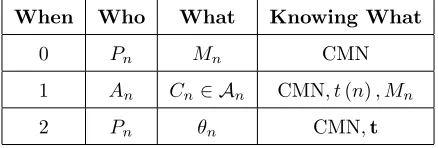
1. Each principal n will design a mechanism Mn = (An,Cn), in which the agent can chooose
an actionan out of setAn . Depending on the agent’s actions in the mechanism, he will be
compensated with a contractC∈ Cn. A contract comprises of shares of the company (1−βn)
and a transfer −αn . A contractCn is hence represented by a pair (αn, βn)∈R×[0,1] and
it will be a function of the action taken by the agent Cn(an). If he does not work he will
get a reservation utility of u≥0 and there will be no profits. From now on, I will slightly abuse notation and indentify an agent’s choice of action in a mechanism, with the resulting contract.
2. Once the shares/wage decisions have been taken, production starts, and agents’ skills will become public.
3. Finally principals can trade their claims to profits αn+βnXn,tn on a market, in which a
riskless assetLis also available in zero net supply.
4. After trading takes place, all uncertainty is realized. Compensation and securities pay off.
When Who What Knowing What
0 Pn Mn CMN
1 An Cn∈ An CMN, t(n), Mn
2 Pn θn CMN,t
Table 1.1: Timing
1.3.3
Strategies and Payoffs
LetT be the set of possible realizations of workers’ skill values and lett= (t1, ...tN) be its generic
element, distributed according toF= (F1, ..., FN)
LetCbe the vector of contracts across the economy.
C={Cn} N
Let θ = (θR|θL) be the portfolio held by an agent. θR is a N-dimensional vector of positive
holdings of theN risky assets, whereasθLis the position an investor holds in the riskless asset.
The ex-ante utility from a portfolioθ fixing the matchingtand the contracts CN, is given by
Up3
n(θ,C,t) =U θ·(~µ(t,C)|1), θ
RΩ(t,C)θR
Demandθ will depend on available assets (and hence con contractsC and their pricesq (but prices are also a function of contracts).
Agents payoffs depend on the action chosen and on the technology of their principal and on their typet:
UA2n=U(Cn, tn)
A Principal’sexpected utility when mechanisms areM, the resulting contracts areC(M) and he holds portfolioθ is
UP1n(M,C(·), θ) =
Z
T
UP3n(θ,C(M),t)F(t)
1.4
Equilibrium
1.4.1
Description
Because individuals take their decisions at each stage looking at the final payoffs, Equilibrium is more easily described starting from the final stage of the game.
Asset Market At this stage the realized skills are observed. There is no asymmetric infor-mation. Principals hold one unit of a security equal to their share of returns in their firm, and a riskless asset is available in net zero supply. The solution concept used here is that of Arrow-Debreu Equilibrium. Since securities payoffs are determined by contractsCand by agents’ skillst, the equilibrium portfolios and prices will be function (θ, q) (C,t),
Contracting, Agents’ turnEach agentAn observes the mechanism he is offered,Mn, and he
except of course Pn. They pick an action maximizing UA2n(·). Their strategies will be functions
an(Mn, tn).
Contracting, Principals’ turnEach principal offers designs a mechanism, without knowing the skills of any agent. However they correctly forecast the strategies of each agent, and the outcome of asset markets, for any possible mechanism. In other words, they can forecast the equilibrium path for all profiles of mechanisms M and types t. Principals at this stage play a game against each other. A mixed strategy forPn is a lottery on possible mechanisms, ˜Mn∈∆ (Mn).
The flow of decisions is described schematically below, and the information available at each stage is summarized by the argument of the strategies.
˜ M
t
→C˜(M,t))→
C
t
→[(θ, q)] (C,t)
Based on this timeline we can write the utility in the first stage in this form:
Vn
˜ Mn|M˜n
=EM˜n
h
UP1n
˜
Mn|M˜−n,C
˜
Mn|M˜−n,˜t
, θCM˜n|M˜−n,˜t
i
Note that ˜tis a random vector andU1
Pn defined above includes an expectation with respect to
its distributionF.
1.4.2
Definition
An Equilibrium consists of
• A trading strategy θ∗
n for each Principal n and prices q∗ ∈ RN+1 such that [θ∗, q∗] (C,t) is
θn∗(C∗,t)∈arg max
θ∈RN++1
UP3
n(θ,C
∗,t)
s.t.
q∗(C∗,t)·θ(C∗,t)≤q∗n(C∗,t)
X
n∈N
θn∗ = [1N|0]
• For each agentAn a strategyCn∗(Mn∗, t(n)) such that
Cn∗(Mn∗, t(n))∈argmax
C∈Cn
UA2n(C, tn)
• For each principalPn,a lottery ˜Mn∗ of deterministic mechanisms such that
supphM˜n∗i⊆arg max
Mn∈M
Vn∗(Mn|M∗−n)
1.4.3
Result
To prove existence of equilibrium I need the following result, the mechanism design classic, “cus-tomized” for this setting in which principals compete with each other..
Let an instance of the previously described economy be G, and the set of its equilibria E(G). Consider now an economyGTwhich is identical in all respects, but where principals are restricted
to offer to agents menus of contracts of size |T|, instead of designing general game forms. I am going to show that E(G) = E GT
. In this way the strategy space of the Principals at the first stage will be finite dimensional.1 The space ofPn’s strategies is going to beM|
T|
n .
Proposition 1. The unrestricted menus economy G and the restricted menu economy GT, have
the same equilibria: E(G) =E GT
Proof. E(G)⊆ E(GT) Consider an equilibrium=M˜,C, θ, qnow construct a strategy profileT
and show it is an equilibrium forGT: Let a menuMT
n of|T| contracts offered in GT
be made
of contracts{(yn)}t∈T:
y(t) =Cn(Mn, t)
For agents, it is an optimal action to choose the contracty(t). Suppose not. Than it would be the case that for somet0
U(y(t0), t)> U(y(t), t) =U(Cn(Mn, t), t)
By constructionCn(Mn, t0)0 played inMp yields the same payoff asy(t0), which contradictsCn
being an equilibrium strategy.
The above described menus are optimal for every principal. Suppose not, then for some principal pthere is a|T|sized menu ˜M0 such that
Vn
M0|M˜T−n> Vn
˜
MT=Vn∗M˜
The equality follows by construction, and sincencould have offered ˜M0in the unrestricted economy, this would contradict being an equilibrium.
E(GT)⊆ E(G)
Consider an equilibrium eT: the agents equilibrium strategies CT are simply the equilibrium
strategies of the real economy, restricted to the domain of |T| sized menus. Moreover, ˜MT, are
equilibrium strategies also in the unrestricted game. Suppose it was not the case, then for somen there is an unrestricted mechanisms lottery ˜M such that
Vn∗( ˜M|M˜−Tn)> Vn∗( ˜MT)
Note that Vn( ˜M|M˜T−n) can be attained by n by offering a lotteries of restricted menus ˜M
0T
made of the following contractsy0:
yn0(t) =Cn(Mn, t)
This implies
Vn∗( ˜M0|M˜T
−n)> Vn∗(M˜ T)
The utility function of a Principal is continuous in the contracts chosen by each type of Agent so it is continuous inCT . To make it continuous in the contracts offered by Principals’ it has to
be that these contracts form Incentive Compatible menus. In other words, menus must come from as subset ofCT such that C1 is always chosen by agent 1,C2 is always chosen by agent 2, and so
on. To achieve this the menu in a contracts must satisfy incentive compatibility constraints. We can be sure that we can restrict attention to these menus because all and only the equilibria of the original unrestricted game are obtained in a game where Principals are allowed to offer only an incentive compatible menu ofT contracts. I will call this economy,GIC.
Corollary 2. The restricted menus economyGand theIC economyGT, have the same equilibria
E(GT) =E(GIC)
Proof. E(GT)⊆ E(GIC) The contracts in the direct revelation menus in the proof of Theorem 1
are Incentive Compatible by construction.
E(GIC)⊆ E(GT) This part of the proof goes as the second part of the proof in Theorem 1: any
outcome that a principal can achieve by menus of sizeT can be achieved by incentive compatibles menu of sizeT.
1.5
Existence of Equilibrium
1.5.1
Assumptions
1.5.1.1 Monotonic Preferences
It is well known that Mean-Variance Preferences are not monotonic. This of course can cause prob-lems for the existence of an equilibrium. In a standard CAPM setting, monotonicity of preferences is solved by imposing a bound on the variance aversion of every individual. I will require agents to not be satiated if they owned every return in the economy, regardless of state. I will then show that this implies they will not be satiated in the asset market of the later stage. It is possible to show that if preferences are monotonic for given returns (µ,Ω), they will be monotonic for the returns induced by any contracts in that economy, (α+βµ, βΩβ0).
Definition 1. LetX be a generic Random Variable on the state spaceS= (s1, ..., sS)taking values
(x1, ..., xS). We say thatU(X)is monotonic if ∂x∂U
Lemma 3. Consider the preferences induced by the utility function
U(X) =E(X)−b
2
E(X)2+V ar(X)
They are monotonic on a set of variablesX defined on a finite state spaceS, if
b <min
X,s
1 X(s)
Proof. The proof amounts to checking (by differentiating) under which conditions ona the utility function is increasing.
Definition 2. Preferences are monotonic for the entire economy ifb < 1
P
nmaxsXn(s)
This definition amounts to stating that if an agent owned the entire returns available to the economy, he would still not be satiated. 2
Lemma 4. If preferences are monotonic for the entire economy with assets characterized by returns (µ,Ω), then they will be monotonic on all feasible portfolios for any contracts (αn, βn)n∈N .
Proof. For preferences to be monotonic for all feasible portfolios it has to be that
b < min
So that the lemma can be restated as
max
Note that the solution to the maximization on both sides is going to be reached at the aggregate market portfolio (θn= 1 for alln) so that the previous is equivalent to
Claim 1
2The definition is equivalent to the less stringentb < 1
maxsPnXn(s) as long as no firms are perfectly correlated
To prove this, note first how Claim 2
max
s αn+βnXn(s)<maxs Xn(s),∀n, αn, βn
Suppose by means of contradiction
∃n, αn, βns.t. max
s −αn+ (1−βn)Xn(s)<0
Which in turn implies
0>−αn+ (1−βn)E(Xn) =E(−αn+ (1−βn)Xn)> EU(−αn+ (1−βn)Xn)
HoweverEU(−αn+ (1−βn)) has to be greater than zero in equilibrium, so that
0> EU(−αn+ (1−βn)Xn)>0
which is impossible. This proves Claim 2 It follows from Claim 2 that
X
n
αn+βnmax
s Xn(s)<
X
n
max
s Xn(s)
Finally
X
n∈N
max
s Xn(s)>
X
n∈N
αn+βnmax s Xn(s)
>max
s
X
n∈N
1.5.2
The existence result
Theorem 5. If preferences are monotonic for the entire economy then there exists an equilibrium in the CAPM contracting economy.
Proof. I am going to use a well known fixed point result by Glicksberg (1952) to show that there is an equilibrium in the first stage of the game, given that the asset market develops as predicted by the CAPM model.
I need to show that
1. The strategy space ∆(MM V) is a convex, compact subset of a locally convex Hausdorff space.
2. The best response correspondence of all principals is upper hemi-continuous, convex valued, and nonempty.
For the first part note that the space of Incentive Compatible menus MM V is a subset of a
Euclidean space. It is closed because it is defined by a finite number of weak inequalities, and it is bounded because the larger set of feasible contracts are bounded. Hence it is compact.
The space of lotteries (identified with Borel probability measures) over these Menus is of course convex. It is also compact with respect to the weak* topology. This space of probabilities is a subset of the space of continuous functionsC(MM V), which is locally convex (and Hausdorff) with
respect to the weak* topology.3
For the second part, convexity of the best response correspondence follows from preferences on random variables being represented by expected utility. I will use Berge’s Maximum theorem to show that it is non empty, compact-valued and upper hemi-continous.
To apply the maximum theorem to individuals’ best response, it has to be that constraints vary continuously with other principals’ strategies, and that the payoff function is continuous in one’s own actions.
First note how the constraints correspondence is constant with respect to other principals strate-gies, and is therefore continuous. Also note how the constraints correspondence maps to the space of Borel probability measures on menus, which is a Hausdorff space as noted above.
We also need to make sure that the payoff function of a principal is continuous in menus. To do this we need to show that
3For a treatment of these and other results on weak topologies, and also to see the theorems of Berge and
1. Payoffs at the market stage are a continuous function of the contracts chosen by agents. 2. The contracts chosen by agents are a continuous function of the menus offered.
Claim 1 By Lemma 4, if the preferences are monotonic for (µ,Ω), they are going to be monotonic for the asset markets resulting from all possible contracts C. Under the present assumptions a CAPM equilibrium exists once contracts are chosen.4 Because in such equilibrium the price of a security can be expressed as qn =αn+βnµn− Nb βn2σ2n+ Σm6=nρmnβmβnσmσn
The indirect utility from a contract profile in the CAPM function is continuous in contracts.
Claim 2 Recall that we can restrict attention to Incentive Compatible menus. If a principal makes a small change to the menu he offers while remaining in this set, every type of agent t , will still find it optimal to pick the contract intended for him, Ct. Hence any small change, will
correspond to a small change in the contract picked by each type of agent.
We can conclude that the indirect utility for a principal facing typet is a continuous function of the menus offered.
Taking expectation with respect toFover these indirect utilities yields a continuous functional on the domain of lotteries on IC menus.
By the maximum theorem the best response correspondence of each player is now UHC and compact valued, which implies that the game best response is as well.
By Glicksberg’s theorem there is a fix point, which is an equilibrium by construction.
1.6
The Insurance Effect of Markets
Throughout this section I will consider the case of firms whose returns are independent.
1.6.1
Utility from Markets
The point of this section is incorporating the outcome of markets in the principals’ utility functions. First consider again what the final holdings are in equilibrium. Every individual will hold the same risky portfolio, an equal fraction N1 of the aggregate endowment, and will spend the rest on the
4In the literature briefly reviewed by Nielsen (1990), one can find many sufficient conditions for the existence of
riskless asset (or short it if their remaining endowment is negative). With this in mind the mean and variance of the portfolio held by the agent is readily computed as a function of contracts. For a general principaliwe have that
• The holding of riskless asset isqi−N1 Pj∈Pqj
• The mean of the risky portfolio is N1 P
j∈N(αj+βjµj)
• The variance of the risky portfolio is 1
N2
and the variance is of course the variance of the risky part N12
P
is the utility a principal obtains from contract α, β when no markets are available, markets will change this into
UM(αi, βi) =
Lemma 6. If the principals are allowed to trade their claims, they will act as if their utility functions were
∂FM
whereas the partial derivatives without markets are
1.6.2
First Best
Theorem 7. When information is complete and symmetric, the variance of optimal contracts is smaller in a large market than without markets. There is a number of principalsN such that
βt∗< βt∗(N), ∀N ≥N
Proof. Consider the problem of a principal.
max
(αt,βt)Tt=1
T
X
t=1
U(αt, βt|t)
s.t. U(−αt,1−βt|t)≥u, ∀t= 1, ...T
Which can be broken into T separate problems
max
(αt,βt)
U(αt, βt|t)
s.t. U(−αt,1−βt|t)≥u
Note that
U(αt, βt|t) =F αt+βtµt, βt2σ
2
t
U(−αt,1−βt|t) =F
−αt+ (1−βt)µt,(1−βt)
2
σt2
Dropping the type subscripts for convenience, we can proceed to solve an individual problem
max
(α,β)
F α+βµ, β2σ2
The first order conditions for this problem amount to
Solving for the optimal contract we have that
βM∗=N U M
Similarly we can “break” the problem with markets in smaller optimizations like the following.
max
(α,β)
FM α+βµ, β2σ2
s.t. F−α+ (1−β)µ,(1−β)2σ2≥u
The first order conditions for this problem amount to ∂LM
Solving for the optimal contract we have that
where
N U MM =Fσ2
−α+ (1−β)µ,(1−β)2σ2FµM α+βµ, β2σ2
DENM =Fσ2
−α+ (1−β)µ,(1−β)2σ2FµM α+βµ, β2σ2
+ FσM2 α+βµ, β
2σ2
Fµ
−α+ (1−β)µ,(1−β)2σ2
By the considerations from Section 1.6.1, we note that, since FσM2 gets arbitrarily small as N
gets large (Nb − b N2 and
1
N2 are arbitrarily small for large enoughN, so isF
M
σ2) . β∗ is arbitrarily
close to 1 in a large economy. Which concludes the proof.
1.6.3
Ordering Types
To solve a risk sharing principal agent problem with multiple types and asymmetric information, I will need to adapt methods use in the contract theory literature.5 I will require that, for any firm,
the type space is ’ordered’ in the sense of Single Crossing Property (ie: any two indifference curves from any two types will cross only once). The following cumbersome notation means exactly this. Given a firm, agents can be ranked (by the slopes of their indifference curves). The ranking need not be the same in every firm.
LetSCP(n) = (1(n),2(n), ..., T(n)) be a function fromNtoTN such thati(n)6=j(n),∀i(n), j(n)∈
1, ...T,∀n.
Definition 3. An economy satisfies Single Crossing Property if and only if there is a function SCP, as defined above such that types µ1(n)), σ1(n)
, ..., µT(n), σT(n)
satisfy Single Crossing Property for alln. That is, if
U2(−α,1−β|t(n))
U1(−α,1−β|t(n))
> U2(−α,1−β|t(n) + 1) U1(−α,1−β|t(n) + 1) ∀t, p, α, β
In the case of quadratic utility,SCP amounts to
5Similar techniques are used in the literature on second order price discrimination. See for example Maskin and
µt−
btσ2t(1−β)
1−bt(−α)−btµt(1−β)
> µt+1−
bt+1σ2t+1(1−β)
1−bt+1(−α)−bt+1µt+1(1−β) Proposition 8. The following cases6 implySCP:
• Agents have the same mean and different variance
• Agents have different mean and the same variance
• Agents generate the same outcomes, but the probabilities of success are different. The proof amounts to the algebra necessary to verify the definition.
The following two facts will come handy for the proving Theorem 11
Fact 9. ∀t,(α, β), U(−α,1−β|t)> U(−α,1−β|t+ 1)
Fact 10. ∀t < s,∀(α, β),(α0, β0) :β ≤β0
U(−α,(1−β)|t)−U(−α0,(1−β0)|t)> U(−α,(1−β)|s)−U(−α0,(1−β0)|s)
1.6.4
Second Best
Theorem 11. If types satisfy Single Crossing Property and markets are large enough, the variance of the average contract is smaller when markets are present.
Proof. The strategy of the proof is to show that -at an optimum- all types shares’ ( (1−β) ) are bounded by the share of the “best” type,t= 1. And that the share of this type become small for large enough market.
A generic principal’s problem is given by
max
(αt,βt)Tt=1
T
X
t=1
U(αt, βt|t)f(t)
s.t. U(−αt,1−βt|t)≥u, ∀t∈ {1, ...T} (IR)
SCP and IC constraints imply by usual arguments that yield that β∗(s) ≥ β∗(t),∀s < t ∈ {1, ...T}. This imply thatβ1≤βt,∀t
Now we have to solve for the contract of type 1. To do this I show that theIC12constraint will
always be binding, and that this is enough to attain the result. The first thing to do is to reduce the set of relevant constraints. Fact 9 implies that
U(−αt,1−βt|t)≥U(−αt,1−βt|T)
This together with IR holding for type T and IC holding for type t with respect to the contracts of type T, implies that IR holds for type t.
In other words, if
U(−αT,1−βT|T)≥u
U(−αt,1−βt|t)≥U(−αT,1−βT|t)
we will also have that
U(−αt,1−βt|t)≥u
We can hence solve the problem without worrying about any of the IR constraints except that of typeT .
We can also infer that ICt−1,t will be binding at an optimum for any t. Suppose that it were
not binding,
U(−αt−1,1−βt−1|t−1)> U(−αt,1−βt|t−1)
U(−αt,1−βt|t)≥U(−αk,1−βk|t),∀k
By Fact 10 it has to be that
U(−αt,1−βt|s)> U(−αk,1−βk|s),∀k≥t,∀s < t
Consider an alternative incentive scheme, which gives less transfer −αs to all typess lower t.
Because their IC constraints for contractsCk, withk > t(ICs,k) are not binding, we are increasing
the maximand while remaining in the admissible set of contracts, which contradicts the original scheme being an optimum.
This and SCP imply that constraintsICt,t−1 will not be binding.
It also implies that no other IC constraint will bind at the optimum. Fact 9,ICt−1,t, andICt,t+1
imply thatICt−1,t+1 is satisfied with a strict inequality.
This means that the only relevant constraints for determining the optimalβ1 are in the form
U(−α1,1−β1|1) =U(−α2,1−β2|1)
I now have to solve a much simpler problem
max
(αt,βt)Tt=1
T
X
t=1
U(αt, βt|t)f(t)
s.t. U(−αT,1−βT|t) =u (IR)
U(−αt,1−βt|t) =U(−αt+1,1−βt+1|t), ∀t∈ {1, ..., T −1} (IC t t +1)
q1Fµ α+βµ, β2σ2
Which yield an expression for 1 identical to the first best case.
β1∗=N U MM
Solving for β1 we obtain a formula similar to the first best case. Just as in the first best case
we can observe thatβ∗ is arbitrarily close to 1 in a large economy, since FσM2 can again be made
arbitrarily small by choosing an appropriately largeN. This bound allows us to reach the result
Claim: P
Lettbe the bijection satisfying SCP for all matches. The claim is equivalent to
and naturally
∀n, ∃N s.t. βn1(n)(N),∀N ≥N ,∀tn
This implies
βn1(n)>X
t
f(tn)βnt,∀N ≥N
and
X
n
βn1(n)>X
n
X
t
f(t)βnt,∀N ≥N
which concludes the proof.
1.6.5
Effects on Welfare and on Asset Markets
As it is usually the case, asymmetric information entails a loss of efficiency.
Corollary 12. Under the assumptions of Theorem 11, the equilibrium is inefficient compared to the complete information case.
Proof. It follows from the fact thatIRT andICT−1,T are both binding thatat least the contract
of typeT is Pareto dominated by the complete information solution of Theorem 7.
Let ∆t(N) = βt∗(N)−βt1(N), where βt1(N) is the first best solution. I will use this as a
measure of inefficiency.
Proof. The proof again leverages on the fact that both first and second best contracts are arbitrarily close to 1 for a large enough markets. The claim is trivially satisfied forβ1∗(N) (the second best
solution, with markets), since it is a Pareto Efficient Contract by construction. Forβt∗(N), t >1
consider ∆t(N) =βt∗(N)−βt1(N), whereβt1(N) is the first best solution with markets. Since
βt∗(N) andβt1(N) both go to one asN gets large, there must be aN such that ∆t(N)<∆t(1)
for allN > N.
1.7
Conclusion
This chapter integrates a model of principal-agent interaction with asset markets. Principals and Agents are randomly matched. Each pair produces random returns, whose distribution is known only to the agent at the contracting stage. Every Principal offers a menu of contracts to the Agent he is matched with, and the Agents make their pick. What marks the difference from the standard contracting model is that Principals have access to an asset market on which they trade their shares of returns.
I present a general framework and define a notion of equilibrium. I prove a revelation principle result, to simplify the study of firms’ structure and prove existence of equilibrium. Under standard assumptions of contract theory, I study the interactions of financial markets on contracts. The existence of markets, induces less risky compensation for agents. In a large market diversification opportunities multiply, and contracts become less and less risky.
Contracting inside firms induces inefficient aggregate risk in an economy, however the size of this inefficiency is reduced by a large enough market. As noted this is a limiting result and it leaves the open question of the behavior in small markets.
Chapter 2
Contracts and Aftermarkets
-Hidden Action
2.1
Introduction
It is well known that financial markets can favor the efficient allocation of resources to production and the sharing of risk. Less is known about their effects on incentives, for those who have limited access to markets. In this chapter I propose a stylized model of firms and financial markets, to capture these effects. The concern here is how different access to markets can affect the incentives to production.
This chapter relates to two branches of economic theory. The literature on Walrasian economies in presence of Moral Hazard issues, and the literature on endogenous securities. I will discuss the fit of my work in these literatures, but first I am going to relate my work to two recent papers, which are particularly relevant to the discussion.
needed, for risk sharing and incentives to coexist? They study several cases, distinguished by the amount of information available for contracting, and for each case characterize the set of securities which allow (constrained) efficiency. In this chapter securities are determined in equilibrium, but they are chosen out of a very simple set. In the future it would be worth describing the endogenous choice of complex securities, to study the efficiency of financial engineering, in terms of incentives and risk sharing, but this is out of the scope of this chapter.
There is by now a vast literature on moral hazard in general equilibrium settings. Helpman and Laffont (1975) and Prescott and Townsend (1984) are among the first to tackle the topic. Their works are concerned with efficiency in exchange and production economies, in which individuals can exert a costly, unobservable payoff relevant action. These papers are the first in a long, but not large, series of works, which extend the study of efficiency to more general economies. My work is different in that I include financial markets, and I trade off some generality for more precise comparative statics results.
A strand of the asset pricing literature looks at asset pricing in the presence of delegated portfolio management (for a survey, see Stracca, 2003). An example of the approach typical in these papers can be seen in Ou Yang’s paper. These studies look at the effects on prices and returns of the classical informational asymmetries phenomena. Moral hazard and adverse selection are largely studied in a CAPM or APT setting, in which a representative principal delegates his investing decisions to an agent. In this literature inefficiencies take the form of deviations from the non-delegated case equilibrium. These deviations can take the form of changes in asset prices and optimal portfolio composition. Besides the different object of interest, the perspective in these works is in a sense opposite of the one taken here. There we have informed parties trading, whereas in the present work it is the uninformed parties accessing markets.
2.2
The Model
This stylized model is meant to capture certain features of interactions within firms and across firms in financial markets. It is helpful to introduce first the model of a single firm, and then proceed to define how they interact.
2.2.1
Primitives
A generic firm i is constituted by a principal-agent pair pi, ai. Each of these firms i generates
random returns. All individuals have identical Mean Variance Preferences over random variables in the familiar form1
U(X) =µ(X)−b
2σ
2(X)
Agents have a reservation utility,u. Agents choose a costly action (which can be interpreted as the effort put into production)ei from the interval E = [e, e]. The cost of effort is a continuous,
strictly increasing real valued functionc(e).
The returns of a firm ˜Xi(ei) depend stochastically on the effort level of the agent employed.
Because of the assumptions on preferences, I can restrict my attention to the mean and the variance of the firm’s returns, and express them as a function of effort levels.
µi(ei)
σ2(ei)
Acontract Ciis a contingent agreement on how to split returns between the Principal and the
Agent forming firmi. I impose the restriction that these sharing rules be affine. IfX is the random variable describing the profits of the firm, an admissible rule describing the principal’s and agent’s
1Note that all the analysis in this paper would apply to the CARA/normal framework, except that conditions for
share must be of the form:
Xai =−α+ (1−β)X
Xpi=α+βX
withα∈Randβ∈[0,1].
A contract Ci amounts to a pair αi, βi. In a binary setting this imposes the restriction that
both shares be increasing in firm’s returns.
Now consider that there are N firms. Let e = [ei(Ci)]1≤i≤N be the vector of efforts, and
C= [Ci]1≤i≤N be the vector of contracts in each firm .
The joint distribution of the vector of firms’ profitsX(e) = [Xi(ei)]1≤i≤N firms’ profits will be
uniquely determined by the effort levels across firms.
µ(e) =
µ1(e1)
.. . µN(eN)
Ωjk(e) =ρjk(ej, ek)σj(ej)σk(ek)
I will denote this vector and matrix asµ(e) and Ω (e).
Principals will have access to a financial market where they can trade their claims to profits and a riskless asset available in zero net supply.
The risky assets available can be described by a random vector,Xp(e, C) = [Xpi(ei, Ci)]1≤i≤N =
[αi+βXi(ei)]1≤i≤N
Because of our assumption on preferences, from now on I will simply identify the principals’ shares with the vector of meansµ(C, e) =α+βµ(e) and the variance-covariance matrix Ω (C, e) = β0Ω (e)β .
2.2.2
Timeline
existence when effort is observable.
CMN will denote the primitives of the game that are common knowledge at every stage, which are:
• The vector of means and the variance-covariance matrix of payoffs as a function of effort levels
µ(·) Ω (··)
• The preferences of individuals (the variance aversion parameterb).
• The reservation utility of agentsu.
The economy reaches its equilibrium in 3 stages.
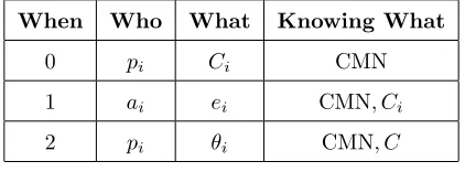
1. Each Principal pi designs a contractCi = (αi, βi). Ci is the set of all possible contracts for
firmi. At this stage every principal knows CMN.
The profile of offered contracts isC={C1, ..., CN} ∈ C= ΠNi=1Ci
2. Each agentai chooses his effort level, based on the contractCi.
A strategy of an agent in firmiis a function of contracts mapping to possible effort levels.
ei:Ci →E
ei:Ci7→ei(Ci)
The strategy profile of all agents can be written as a vector of functionse= [ei(Ci)]1≤i≤N of
contracts offered.
cumulative distribution function induced by the beliefs on firmiunder contractCi. Principal
j holdsθi
j shares of firmiand the price of the stock of firm iisqi
This table summarizes the choices each individual faces at a given time, and the information available to them.
When Who What Knowing What
0 pi Ci CMN
1 ai ei CMN, Ci
2 pi θi CMN, C
Table 2.1: Timing
2.2.3
Payoffs
Letθbe the portfolio held by an agent. Let θ= (θR|θL) Where θR is anN-dimensional vector of
positive holdings of theN risky assets, whereas θL is the position an investor holds in the riskless
asset.
The ex-ante utility from a portfolioθ fixing the contractsC and effort choicese, is given by
θ·(µ(C, e)|1)−b
2θ
0
RΩ(C, e)θR
However principals don’t observe the efforts e so they evaluate utility of portfolios based on contractsC and the beliefs they induceγ(·|C)
Upi(C, θ, γ) =
θ·
Z
E
µ(C, e|1)dγ(e|C)−b
2
Z
E
θ0RΩ (C, e)θR+
µ(C, e)−
Z
E
µ(C, e)
2!
dγ(e|C)
Demand θ will depend on available assets and their prices (but prices are also a function of contracts).
Agents payoffs depend on the effort chosen and the contract in place.
Uai(Ci, ei) =µi(Ci, ei)−
b 2σ
2
i (Ci, ei)−c(ei)
2.3
Equilibrium
2.3.1
Description
Because individuals take their decisions at each stage looking at the final payoffs, Equilibrium is more easily described starting from the final stage of the game.
Asset Market Principals hold one unit of a security equal to their share of returns in their firm, and they all have the same information. Because all individuals have the same beliefs the solution concept used here is that of Arrow-Debreu Equilibrium. The equilibrium portfolios and prices will be based on expected payoffs induced byC. They will be a function (θ, q) (C, γ(e|C)).
Contracting, the Agents’ turnEach agentai observes the contract he is offered,Ci, and he
knows his own type and the technology of the principal. This is all the payoff relevant information, so every agent is facing a choice between lotteries, and he is not playing against other players. They simply choose an effort level maximizingUai(·). As noted their strategies will be functionsei(Ci).
Contracting, the Principals’ turnEach principal designs a contract. They correctly conjec-ture the action of each agent, and the outcome of asset markets, given contracts. They can forecast the equilibrium path for all possible strategy profiles. Hence, this stage can be seen as a game principals play against each other. I will focus on equilibria in pure strategy equilibria (and show their existence).
The flow of decisions is described schematically below, and the information available at each stage is summarized by the argument of the strategies.
Vpi(C) =Upi(C, θ(γ(e|C)), γ(e|C))
2.3.2
Definition
An Equilibrium consists of
• A trading strategy θ∗i for each Principal pi and prices q∗ ∈ RN such that [θ∗, q∗] (C, γ) is
an Arrow-Debreu Equilibrium for the asset market when contracts are C . Each princi-pal is endowed with one unit of one asset so that the endowment of principrinci-pal pi is wi =
[0,0, ...,1, ...,0,0] with 1 being in thei-th position.
θi∗(C, γ(e|C))∈arg max
θi∈RN++1
Upi(C, θi, γ(e|C))
such that
q∗(C, γ(e|C))·θi(C, γ(e|C))≤q∗(C, γ(e|C))·wi
X
i∈N
θ∗i = [1N|0]
• Beliefsγ∗(e|C) such that
supp(γi∗)⊆argmax
˜
ei∈E
Uai(Ci,e˜i)
• For each agentai a strategye∗i(Ci) such that
ei(Ci)∈argmax ei∈E
Uai(Ci, ei)
• For each principalpi, a contractCi∗ such that
Ci∗∈arg max
Ci∈Ci
Vi∗ Ci, C−∗i
=Upi Ci, C
∗ −i
, γ∗ e|Ci, C−∗i
, θ∗ Ci, C−∗i
, γ∗ e|Ci, C−∗i
2.4
Existence of Equilibrium
2.4.1
Assumptions
2.4.1.1 Monotonic Preferences
It is well known that Mean-Variance Preferences need not be monotonic. This could pose problems for the existence of equilibrium. In a standard CAPM setting, monotonicity of preferences is solved by imposing a bound on the variance aversion of every individual. Because I restrict attention to linear contracts, it is possible to show that, if preferences are monotonic for given returns, they will be monotonic for any prevailing contracts.
Definition 4. LetX be a generic Random Variable on the state spaceS= (s1, ..., sM)taking values
(x1, ..., xM). U(X)is monotonic if ∂x∂U
i >0,∀i.
Lemma 14. Consider the preferences induced by the utility function
U(X) =E(X)−b
2V ar(X)
They are monotonic on a set of variablesX defined on a finite state spaceS, if
b <min
X,s
1
|xs−µX|
Proof. The proof amounts to checking (by differentiating) under which conditions onbthe utility function is increasing.
Lemma 15. If preferences are monotonic for all feasible portfolios in an economy with assets char-acterized by returns(µ,Ω), then they will be monotonic on all feasible portfolios for any contracts (αi, βi)i∈N .
Proof. For preferences to be monotonic for all feasible portfolios it has to be that
b < 1
|maxP
i∈Nθixi−Pi∈Nθiµi|
= 1
|maxP
i∈Nθi(xi−µi)|
Where the max is taken across portfoliosθsuch thatθi∈(0,1) and outcomesxi∈supp(Xi). Note
that
X
i∈N
θi[(−αi+ (1−βi)]xi−[−αi+ (1−βi)µi)]
=X
i∈N
θi((1−βi)xi−(1−βi)µi)
=X
i∈N
θi(1−βi) (xi−µi)
I claim that
max|X
i∈N
θi(1−βi) (xi−µi)| ≤max|
X
i∈N
θi(xi−µi)|
Note that the solution to the maximization on both sides is going to be reached at the aggregate market portfolio so that the previous is equivalent to
max|X
i∈N
(1−βi) (xi−µi)| ≤max|
X
i∈N
(xi−µi)|
Since it will also be the case that at the maximum all the xi’s chosen will be greater (or smaller)
than theµi’s so that
maxX
i∈N
(1−βi)|(xi−µi)| ≤max
X
i∈N
|(xi−µi)|
Observing thatβi∈[0,1] concludes the proof
Assumption 1. For a given set of assets, for every individuali, their risk tolerance parameter bi
lies on the interval 0, b
, whereb= minX,s|x 1
s−µX|
This ensures that everyone’s preferences will be monotonic.
2.4.1.2 Cost and Productivity of Effort
introducing further randomizations (such as some individual playing a mixed strategy) is undesirable in many ways. 2 Moreover, if only one effort choice is optimal for an agent, then principals can
correctly infer the equilibrium effort by observing contracts. To achieve this I need each agent’s objective function to be concave in effort for any possible contract (α, β).
Assumption 2. 1. The cost function of an agentc(e)is strictly increasing and strictly convex. ∂c
∂e >0, ∂2c ∂e2 >0
2. The effect of effort on the mean distribution of returns is such that utility is strictly increasing and concave in effort, the effect on the variance is strictly decreasing and convex for all 0, b
∂µ ∂e >0,
∂2µ ∂e2 ≤0
∂σ2
∂e <0, ∂2σ2
∂e2 >0
3. Moreover, I require the effect of effort on the variance to be bounded relative to the effect on mean returns.
µe>|σe2|
|µee|>|σ2ee|
Note how the first set of conditions implies that
∂µX(e)
∂e − b 2
∂σ2
X(e)
∂e >0 ∂2µ
X(e)
∂e2 −
b 2
∂2σ2
X(e)
∂e2 <0
Lemma 16. Under Assumptions 1 and 2, the solution to the agent’s problem,e∗(β) is
• unique
• continuous
• decreasing
The First Order Conditions of these problems amount to
(1−β)µe(e)−
b
2(1−β)
2
σe2(e)−ce(e) = 0
Uniqueness. It follows from Assumption 2 that this derivative is a strictly decreasing function on E = [e, e]. To see this note that by, Assumption 2, concavity is guaranteed for any risk tolerance parameter in the interval 0, b. This implies that the assumptions for derivatives will also be true for
forβ between 0 and 1. This and the fact that cost is convex imply uniquness of the solution. Continuity. forβ in [0,1) follows from the implicit function theorem. Whenβ= 1 the optimal effort ise.
Corollary 17. In equilibrium, principals correctly conjecture the equilibrium effort of agents.
γi∗(ei|Ci) = 1, ei≥e∗i(Ci)
= 0, ei< e∗i(Ci)
This follows immediately from the definition of equilibrium and Lemma 16. By doing this, I am removing one potential layer of randomization. The objective function of a principal at the first stage will be.
Lemma 18. The best response of a principal is single valued.
Proof. The proof amounts to showing that every principal is maximizing a strictly concave function on a convex set. Once the reaction function of the agent in incorporated in his individual rationality constraint, the resulting set need not be convex. However, by substituting theIRconstraint in the objective function, I define a simple maximization problem onβ in [0,1] . By Assumption 2.3, the resulting maximand is a strictly concave function.
Let’s start by studying the sign of the second derivative with respect to β of the objective function of a generic principali. To make the proof more readable I abuse notation and suppress all theisubscripts.
IfP
j6=iρijβjσj
is positive, it follows from Assumptions 2 and 1 that the addend on each line is negative. If the coefficient is negative we can observe that Nb − b
N2
P
j6=iρijβjσj
is smaller than 1, by Assumption 1. This together with Assumption 2.3 implies that all the addends are negative as desired.
Let’s now study the second derivative of the IR constraint reducing it to
e2β
Substituting the first term witheβ
The last term is problematic because it is positive.
Substituting forαin the objective function, we have V (β) defined on [0,1] The derivatives of this function will be given by
eβ
The term multiplying eβ needs to be positive. Inspecting the expression, it is clear that the
“worse” possible scenario is whenβ = 0 andP
j6=iρijβjσj
takes the lowest possible value (the largest negative value). As noted above Nb − b
N2
P
j6=iρijβjσj
is smaller than 1. A sufficient condition for this expression to be always positive is
µe+bσe2+bσe>0
But this is implied by Assumption 2.3 . The second derivative of V is hence negative, which concludes the proof.
2.4.2
Existence
Theorem 19. If the mean-variance preferences are monotonic for an asset market economy char-acterized by the mean vector µand variance-covariance matrix Ω then there exists an equilibrium in the CAPM contracting economy.
Proof. Because the Markowitz preferences are not expected utility -and they also fail to satisfy the ’betweenness axiom’ (see Dekel, Safra, Segal (1991) -the best response correspondences of individuals would not be convexified by allowing for lotteries. This makes using the fixed point theorems by Glicksberg or Kakuthani impossible. I will instead show that the game can be reduced to a one-shot game in which principals have acontinuousbest response functionfunction and apply Brouwer’s fixed point theorem.
Upi =qi−
P
i∈Nqi
N +
P
i∈Nµi
N −
b 2
1’Ω1
N2
As noted earlier prices and returnsq, µ,Ω are all continuous functions of contractsC and efforts e.
Agent’s Turn: Effort Choice. By Lemma 16 effort levelseare continuous functions of contracts C, hence the final utility of a principal can be described as a continuous function of contractsC .
Principals’ Turn: Contract Design. By Lemma 18 the Principals’ problem is equivalent to a strictly concave optimization so that their best response function is always unique. By the maximum theorem it is also continuous.
The strategy space Cis a rectangle, which is a convex, compact subset ofR2N .
This satisfies the hypotheses of Brower fixed point theorem. There exist a fix pointC∗ which determines uniquely equilibrium efforts, beliefs, prices and portfolios. C∗, e∗, γ∗, θ∗, q∗ form an equilibrium by construction.
2.5
The Insurance Effect of Markets - Moral Hazard
Consider the following special case. Individuals are identical in the sense that they all have Markowitz type of Mean-Variance preferences, and they all have the same risk tolerance coeffi-cient. Technologies have different variances (denoted by σ2
i and different correlation coefficients
ρij). The mean returns of firms are determined by the effort of agents ei, specificallyµi(ei) =ei.
Cost is quadraticc(ei) =2ce2i
2.5.1
First Best Equilibrium
For the purpose of having a benchmark for optimal risk sharing and optimal effort, let’s have a look at the first best (observable action) case.
2.5.1.1 No Markets
max
α,β,e α+βe−
b 2β
2σ2
such that −α+ (1−β)e−b
2(1−β)
2
σ2− c
2e
2≥u (IR)
The optimal solution, action and contract is
e∗=1 c (α∗, β∗) =
−b
8σ
2+u,1
2
Proof. Substitute forαin the objective function to obtain
max
β,e U(β, e) = (1−β)e−
b
2(1−β)
2
σ2−c
2e
2
i −u+βe−
b 2β
2σ2
which yields the first order conditions ∂U
∂β =a(1−β)σ
2−aβσ2= 0
∂U
∂e = 1−ce= 0 Which give the solution.
2.5.1.2 Financial Markets
Now I consider the case of many firms. To do this I solve the optimization problem of an arbitrary principal, who has now access to a financial market. The form of the utility function follows from similar considerations as in the hidden type case seen in Chapter 1..
αi+βiei+
Proof. Using the CAPM pricing formula, the riskless share of principal from firmi
αi+βiµi−
Each principal holds a fraction of the aggregate portfolio, in particular he holds a random variable from which he gets utility
P
max UiM KT (αi, βi) =
The optimal solution, action and contract is
eM KTi =1
Proof. Substitute forαi in the objective function to obtain
max
which yields the first order conditions ∂UM KT Which give the solution.
As noted in the case of hidden type economies, the effect of markets is that principal acts as if they were less risk averse. This changes the optimal risk sharing.
To better understand the effects of markets, let’s focus on the special case in which all technolo-gies are identical and so are their correlation coefficients.
σi =σj=σ,∀i, j
ρij =ρ,∀i, j
The symmetric solution in this case is
β= 1−
(N−1)2
N2 ρβ
1 + 2NN−21
So that in equilibrium
βM KT = N
2
N2+ 2N−1 +ρ(N2−2N+ 1)
Note how, unless there is perfect correlation, in equilibrium, a principal always take more risk than in the no the market case βi= 12
. In fact the equilibrium contracts will be identical to the no market case only if technologies are perfectly correlated (ρ= 1) .
∀ρ <1, βM KT < N
2
N2+ 2N−1 +N2−2N+ 1 =
1 2
2.5.2
Second Best Equilibrium
2.5.2.1 No Markets
Let’s now turn to the more interesting case of unobservable actions. How do markets affect the equilibrium actions and returns? Here the decisions on risk sharing and effort are interdependent.
max
To simplify the problem let’s start by solving the problem of an agent facing a given contract (α, β) .
Because Individual Rationality can be optimally attained with the transferα, the optimal action ecan be obtained from the first order condition of the agent problem.
(1−β)−ce=o
Plugging e∗ = 1−cβ back into the Principal’s objective function and the agent’s IR constraint yields the following problem
max
β= bσ
2
2bσ2+1
c
e= bcσ
2+1
c
2bσ2+ 1
Proof. Again substitutingαresults in
max
α,β β
1−β c
− b
2β
2σ2+(1−β) 2
c −
b 2(1−β)
2σ2−(1−β) 2
2c −u Differentiating with respect toβ gives the first order condition
−2bβσ2+bσ2−β
c = 0
The solution follows immediately from this and the fact thate= 1−cβ Note howβ < 1
2 . Risk sharing is distorted to give the proper incentive to the agent. Note that
β >0, so thate < 1c. Because there is a trade-off between incentivizing the agent and optimally sharing risk between two risk averse individuals, the first best cannot be achieved.
I am now going to analyze how markets affect this tradeoff.
2.5.2.2 Financial Markets
max UiM KT(αi, βi) =
The solution is now
βiM KT =
In the symmetric case
βM KT = bσ
2N2
bσ2N2+ 2N−1 +ρ(N−1)2+N2
c
The solution differs from the first best case because of the N2
c term added to the denominator.
So the equilibrium securities will be less risky than in the first best case. Moreover as observed for the non market case, the equilibrium effort is lower than at the optimum. BecauseβM KT is again
increasing inN, the equilibrium effort and hence returns are decreasingN.
In a fully symmetric case this result holds for every firm. This will not be the case if we drop the assumption of symmetry. However, the result will still hold in the aggregate in an economy where firms marginal distributions are identical, but not their conditionals. In other words I al-low for different ρij coefficients in the variance covariance matrix. This means that while every
Proposition 21. Consider an economy with identical marginal distributions characterized by mean ei, varianceσ2, cost of effort c2e2. The aggregate output with markets is lower than the aggregate
output without markets.
ΣNi=1e∗i ≥ΣNi=1eMi
with the inequality holding strictly unlessρij = 1,∀i, j
Proof. Claim 1.
ΣNi=1e∗i ≥ΣNi=1eMi ⇐⇒ ΣNi=1βi∗≤ΣNi=1βiM
To see this note that
ΣNi=1e∗i ≥ΣNi=1eMi ⇐⇒
ΣNi=1(1−β
∗
i)
c ≥Σ
N i=1
1−βM i
c ⇐⇒
ΣNi=1(1−β∗i)≥ΣNi=1 1−βiM
⇐⇒
ΣNi=1βi∗≤ΣNi=1βiM
After estabilishing the above inequality. Observe that under the assumptions
βi∗= 1 2 + cbσ12
βiM = 1−
N−1
N2 Σj6=iρijβjM
1 + cbσ12 +
2n−1
N2
I need to prove that
ΣNi=1 1 2 + cbσ12
≤ΣNi=11−
N−1
N2 Σj6=iρijβjM
1 + 1
cbσ2 +
2N−1
N2
ΣNi=1βi∗≤ΣNi=1βiM ⇐⇒
Note that the denominator of βM
i can be rewritten as 2 +
1
cbσ2 −
(N−1)2
N2 . The first inequality
amounts to
Simplifying the last inequality
N(N−1)−
Claim 2 immediately follows.
To conclude the proof, suppose by means of contradiction that the proposition did not hold, by Claim 1, ΣN
i=1β∗i >ΣNi=1βMi . By claim 2 this implies that ΣNi=1βi∗<ΣNi=1Σj6=iN1−1ρijβjM
Then it should be that
ΣNi=1Σj6=i
1 N−1ρijβ
M
j >ΣNi=1βiM
This can be rewritten as
which is impossible sinceρij <1,∀i, j
Financial Markets change the terms of risk sharing inside firms. Unlike the first best case, this has an effect on the equilibrium action, because it is exactly risk providing incentives for the agent to exert some positive effort. As the relative terms of risk sharing change, we move further away from the case in which the agent is risk neutral and optimal effort is obtained.
In this case, it seems markets reward firms for variance against returns, but that is not exactly the case. Markets reward firms for providing opportunities for hedging and diversification in specific states of the world.
To get a better intuition for this result, suppose there is a state spaceS={SU N, RAIN}
Consider a principal owning the an ice cream factory. Her firm returns can take two values, x+e > x+e respectively, in state SU N and in state RAIN . The security she is selling to the market will returnα+βx+βeandα+βx+βe. When designing an incentive contract she is playing with 3 variablesα, β, e. When markets are not available, the underlying state representation does not matter, the solutionα∗, β∗, e∗ will be some tradeoff between risk sharing and incentives (increasingβ decreasese and viceversa . However consider now what happens if there is another firm, whose securities returnα0+β0x+βe0 when the state isRAIN andα0+β0x+βe0 when the
3 components of her contract
∆α RAIN : ∆α SU N: ∆α ∆β RAIN : ∆βx+ ∆βe SU N: ∆βx+ ∆βe ∆e RAIN : ∆eβ SU N : ∆eβ
Note howβ is the only component of the contract which has a different effect in different states, and specifically it provides more exactly where needed: in state SU N. On the other hand, the agent, who does not access markets, values equally returns in equally likely states (risk aversion would make returns in RAIN more valuable, if anything). Because markets change the relative value of returns in difference states for principals, the solution under markets will exhibit different risk sharingβM KT > β∗ and consequently lower equilibrium efforteM KT < e∗.
Understanding this effect allows one to construct an example in which contracts and firms’ output are affected in the opposite way as described above.
Consider an economy with two types of firms (50 of each kind). The low variance firms have variance .25, the high variance firms have variance 1. They are perfectly positively correlated ρij = 1,∀i, j. Risk aversion is.2, cost of effort is.5 . The average output without markets is given
by 10656. Numerical evaluation yields an average output 2.11 .
2.6
Conclusion
This chapter integrates a model of principal-agent interaction with asset markets. Each pair/firm produces random returns, whose distribution depends on agents’ efforts. Every Principal offers a contract to the Agent he is matched with, and the Agents choose their costly action. What marks the difference from the standard contracting model is that Principals have access to an asset market on which they trade their shares of returns. This assumption is meant to capture the limited degree of access to financial markets, available to the average worker, who cannot entirely insure his labor risk.
I present a unified framework for which I define a notion of equilibrium and prove its existence and uniqueness. Under standard assumptions of contract theory, I study the interactions of financial markets on contracts.
On one hand, Moral Hazard inside firms induces suboptimal aggregate risk in an economy. On the other hand, introducing markets for principals, has ambiguous effects. If the marginal distributions of returns of firms are identical, markets will induce lower production levels. I construct an example, where asymmetry of marginal distributions and high degree of correlations induces riskier compensation packages in certain sectors and a positive effect on aggregate output.
Interesting directions for the future include making welfare comparisons with the case where workers can (at least partially) access financial markets, and making the decision of entering markets endogenous in a non trivial way (making access costly).
2.7
Appendix
2.7.1
Preferences
Consider two random variables X1 andX2. We will have that
U(X1) =E(X1)−
b
2V ar(X1) U(X2) =E(X2)−
b
2V ar(X2)
Now consider a mixture with probabilitypof X1 and X2. which we will