Limit Cycle Characterization of an Aeroelastic Wing in a Bluff Body Wake.

(1)

ABSTRACT

GIANIKOS, ZACHARY NILE. Limit Cycle Characterization of an Aeroelastic Wing in a Bluff Body Wake. (Under the direction of Dr. Matthew Bryant).

This paper presents an experimental investigation aimed at characterizing the kinematics

of a pitching-heaving aeroelastic wing placed downstream of a rectangular bluff body. The

influence of the bluff body wake on the wing is two fold: a viscous wake which produces a

velocity deficit downstream and an oscillating induced velocity field due to periodic vortex

shedding. The latter effect is the focus of this paper, specifically, the interaction between the

wake frequency and the wing limit cycle oscillation (LCO) frequency. Wind tunnel

experi-ments showed that the presence of the upstream bluff body causes modulation of the LCO

amplitude. The modulation resembles a beat phenomenon, however the modulation frequency

is related to the third harmonic frequency of the LCO oscillation rather than the fundamental

frequency. The modulation behavior also differs from that of a beat in that the spectral

con-tent contains sideband frequencies, characteristic of a multiplication between a carrier wave

and a modulation wave rather than a simple sinusoidal superposition. Additionally, the

stream-wise spacing between the bluff body and the wing significantly influences the wing kinematics,

with a closer spacing between the two bodies increasing the intensity of the amplitude

mod-ulation. For shedding frequencies sufficiently close to the LCO third harmonic, reducing this

streamwise distance is shown to induce an alternation between two distinct modes of amplitude

(2)

(3)

Limit Cycle Characterization of an Aeroelastic Wing in a Bluff Body Wake

by

Zachary Nile Gianikos

A thesis submitted to the Graduate Faculty of North Carolina State University

in partial fulfillment of the requirements for the Degree of

Master of Science

Aerospace Engineering

Raleigh, North Carolina

2019

APPROVED BY:

Dr. Ashok Gopalarathnam Dr. Lawrence Silverberg

(4)

BIOGRAPHY

Zach Gianikos received a B.S. in Aerospace Engineering from North Carolina State University

in 2017. His research interests include applied aerodynamics, structural dynamics,

aeroelastsic-ity, and experimental UAV development. Outside of the lab he enjoys camping, hiking, flying

(5)

ACKNOWLEDGEMENTS

I would like to gratefully acknowledge funding support from by the Air Force Office of

Sci-entific Research under award number FA9550-17-1-0301, monitored by Dr. Gregg Abate as

well as additional support from the National Science Foundation under Award No. ECCS –

1509592 and program officer Radhakisan S. Baheti.

Throughout this process I have been extremely lucky to receive personal and academic

support from professors, friends, family, and fellow students alike. I consider the teamwork

mentality of the iSSRL to be a significant factor in my research success over the past two

years. I felt at home from day one and no matter how many questions I had (of which there

were plenty), the team was always more than happy to share their knowledge. Finally I would

like to thank Dr. Bryant and Dr. Gopalarathnam in particular for their guidance and receptivity

(6)

LIST OF TABLES

Table 2.1 Mass and dimensional properties . . . 6 Table 2.2 Bluff body spatial configurations . . . 8

(8)

LIST OF FIGURES

Figure 2.1 CAD model of aeroelastic apparatus . . . 5 Figure 2.2 Photograph of aeroelastic apparatus shown with bluff body mounted

upstream . . . 7 Figure 2.3 Schematic of bluff body spatial configuration (wing deflections not to

scale) . . . 7

Figure 3.1 Spring torque measurements with load cell compared to Eqn. 3.3 . . . . 11

Figure 4.1 (a) Non-dimensional mean heave amplitude and (b) mean pitch am-plitude vs windspeed for no-bluff-body case. Error bars represent one standard deviation. . . 14 Figure 4.2 Pitch angle time histories for no-bluff-body case. . . 15 Figure 4.3 (a) Fundamental LCO frequency for pitch and heave vs windspeed and

(b) mean pitch-heave phase difference ¯φθ,hvs windspeed for no-bluff-body case. . . 16 Figure 4.4 Pitch angle PSD plotted vs windspeed for no-bluff-body case (PSD

magnitude = arbitrary log scale) . . . 17 Figure 4.5 Pitch angle time histories forX_b/D= 4.3 case. . . 18 Figure 4.6 Pitch angle PSD plotted vs windspeed forX_b/D= 4.3 case (PSD

mag-nitude = arbitrary log scale) . . . 19 Figure 4.7 Pitch amplitude distributions for (a) no-bluff-body, (b)X_b/D= 6.5, (c)

X_b/D= 5.6, (d)X_b/D= 4.3. . . 21 Figure 4.8 Pitch amplitude CV contours for (a) no-bluff-body, (b)X_b/D= 6.5, (c)

X_b/D= 5.6, (d)X_b/D= 4.3. . . 23 Figure 4.9 Time-frequency content of pitch angle envelope (bottom) with

corre-sponding pitch angle time history (top) for (a)X_b/D= 6.5, (b)X_b/D= 5.6, and (c)X_b/D= 4.3 where f_shed/f_LCO=2.8. . . 24 Figure 4.10 Time-frequency content of pitch angle envelope (bottom) with

corre-sponding pitch angle time history (top) for (a)X_b/D= 6.5, (b)X_b/D= 5.6, and (c)X_b/D= 4.3 where f_shed/f_LCO=3.25. . . 27 Figure 4.13 Phase portraits for (a) no-bluff-body (U∞=10.4m/s) and (b) Xb/D=

(9)

Figure 4.14 θ (top) andφθ,h(bottom) vs time for (a) no-bluff-body (U∞=10.4m/s) and (b)X_b/D= 6.5, (c)X_b/D= 5.6, and (d)X_b/D= 4.3 (f_shed/fLCO=2.9). 31 Figure 4.15 Phase portrait of θA vs φθ,h for no-bluff-body (U∞ =10.4m/s) and

X_b/D= 6.5 (f_shed/f_LCO=2.9). . . 32 Figure 4.16 (a)φθ,hand ¯Pnetvs time and (b)θAvs time forXb/D= 6.5, fshed/fLCO=

(10)

LIST OF SYMBOLS

β fitting parameter for softening pitch stiffness model

φθ,h pitch-heave phase difference[◦]

ρ freestream air density [kg/m3]

θ,θA pitch displacement and pitch amplitude, respectively[◦]

AR wing aspect ratio

b airfoil semi-chord length [m]

c airfoil chord length [m]

C₁,C₂,C₃ fitting parameters for softening pitch stiffness model

c_h,c_p viscous damping coefficient for heave and pitch, respectively [kg/s]

C_L,C_m lift and pitching moment coefficients, respectively

D bluff body characteristic length (short side) [m]

E,T,U total, kinetic, and potential energy, respectively [J]

F_f force due to kinetic friction in the heave degree of freedom (DOF) [N]

f_LCO fundamental frequency of limit cycle oscillation [Hz]

f_shed bluff body shedding frequency [Hz]

(11)

K_h effective heave stiffness [N/m]

K_θ_A,K_θ_B,K_θ_C effective pitch stiffness for linear, hardening, and softening regimes,

respec-tively [Nm/rad]

M_f moment due to kinetic friction in the pitch DOF [Nm]

m_W,m_T wing mass (rotating components), and total mass (all moving components), respectively [kg]

M_θ restoring moment due to structural pitch stiffness

P power [W]

S wing planform area [m2]

St Strouhal number

t time [s]

U_∞ freestream wind speed [m/s]

W_A,WD net work done by aerodynamics and work done by structural damping, re-spectively [J]

X_b streamwise distance between bluff body trailing edge (TE) and wing leading edge (LE) [m]

x_p non-dimensional pitching axis location (chord length fraction from LE)

x_θ non-dimensional distance (by semi-chord) from pitching axis to rotational

(12)

Chapter

1

Introduction

Unsteady wing-wake interaction research has undergone profound growth in recent years as

researchers utilize knowledge of wake impingement to develop new multi-vehicle flight

forma-tions, design novel micro-air vehicles [26], and leverage inspirations from biological swimmers

and flyers [13]. Examples of such interactions include close formation flight [2], wake-induced

flutter [5, 23, 12], aerial refueling [3], and fish schooling dynamics [21]. Although diverse in

applications, the fundamental thread through this area of research is the characterization of

in-teractions between unsteady wakes and lifting bodies. Given the ubiquity of wake impingement

in real systems, these interactions are pertinent in the characterization of limit cycle oscillations

(LCO) of nonlinear aeroelastic systems.

Previous experimental and computational studies have addressed the characteristics and

mechanisms of aeroelastic LCO for undisturbed flow conditions [22, 19, 6]. The effect of

up-stream flow disturbances on the kinematic behavior of wings undergoing LCO, however, has

received less attention. In studies of nonlinear aeroelastic systems, researchers found that the

wing response dynamics depend heavily on the inflow conditions. Poirel et al. [20] found that

(13)

speed to a point lower than that for the non-excited case. In addition to reducing the flutter

speed, the damping is also diminished for airspeed below the flutter point. In a numerical study

of an aeroelastic airfoil with varying inflow, Venkatramani et al. [24] demonstrated

intermit-tency, a phenomenon generally discussed in the context of nonlinear dynamical systems [8, 7].

Intermittency is characterized by an alternation between qualitatively different states, usually

in the vicinity of a stability boundary. Venkatramani et al. [24] showed that fluctuations of the

flow velocity over large time scales produced an "on-off" intermittency in which the system

al-ternated between states of stability and instability about the flutter point. However, for shorter

period velocity fluctuations, the system underwent amplitude-modulated oscillations without

fully regaining stability.

The previously mentioned studies [20, 24] have considered effects of either isotropic

turbu-lence or purely longitudinal freestream velocity fluctuations. Although useful

conceptualiza-tions, these conditions are rarely encountered outside of wind tunnel experiments or numerical

simulations. Several studies in past decades have examined the effect of impinging Kármán

vortex streets on downstream airfoils undergoing prescribed motion. These flow structures

produce relatively high anisotropy and large-scale unsteadiness and therefore, are analogous

to scenarios where the flow is disturbed by an upstream structure. One such study comes from

Chen and Choa [4], who examined the effect of a wake shed from a cylindrical rod upstream

of a NACA 0012 airfoil pitching upward at a constant rate and performed measurements of the

unsteady forces acting on the airfoil. Chen and Choa [4] reported that the peak suction pressure

at the leading edge of the airfoil with the cylinder placed upstream was increased by as much as

50% compared to the undisturbed case and that the peak suction was reached at a larger angle

of attack. They attributed this effect to the upstream disturbance acting as a vortex generator

that energizes the boundary layer, causing earlier turbulent transition and delayed separation

(14)

re-garding the effect of an impinging wake from a bluff body on the dynamic stall characteristics

of a sinusoidally pitching airfoil using direct numerical simulation. They concluded that the

impinging wake largely affects the forces and moments acting on the airfoil by altering the

formation of vortex structures. For the conditions investigated, Merrill and Peet [17] concluded

that dynamic stall for a pitching airfoil occurs later in the pitching cycle when in the presence

of a turbulent wake due to the delayed formation and detachment of the DSV. Both of these

studies were successful in identifying aerodynamic mechanisms of the impinging wake

struc-tures; however, since the airfoils in both cases underwent prescribed motion, they do not reveal

effects on the aeroelastic kinematics and dynamics.

The aim of this paper is to investigate the kinematic response of an aeroelastic wing system

undergoing LCO in the presence of an impinging bluff body wake. Experiments are first

con-ducted without the presence of an upstream bluff body to establish the baseline case. Then, tests

with the bluff body positioned upstream are performed, varying two parameters: the bluff body

shedding frequency, which is varied implicitly via the freestream velocity, and the streamwise

(15)

Chapter

2

Experimental Methods

2.1 Aeroelastic Apparatus Design

A two-degree-of-freedom aeroelastic apparatus was constructed to investigate the effects of

wing-wake interaction phenomena (Fig. 1). The wing is a 3D printed symmetric version of the

SD 7003 with a chord length (c) of 150mm and aspect ratio (AR) of 4. Based on the results

of Visbal and Garmann [25], endplates are attached to the tips of each wing to emulate 2D

flow conditions. The endplates extend one chord length forward and aft of the wing section.

The pitching axis was located at the mid-chord position for the experiments discussed in this

paper. The aeroelastic system is supported within the wind tunnel test section by an external

box structure which acts as a mechanical ground, isolated from the wind tunnel. The wing is

supported by upper and lower PBC Linear guide rails and carriages (Fig. 2.1). Linear extension

springs provide elastic restoring force and moment for both the heave and pitch degrees of

freedom. A set of springs are attached to a cable-pulley system to create a restoring moment

for the pitch degree of freedom. The spring stiffness properties are characterized later in Section

(16)

Ballast

Rotary encoder Pulley

Linear encoder Extension eprings

Upper carriage assembly

Endplates

Flow direction

Lower carriage assembly

Figure 2.1CAD model of aeroelastic apparatus

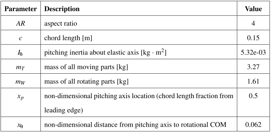
Table 2.1 provides the mass and geometric system properties. These values were obtained

via direct measurement except for the center of mass (COM) and moment of inertia (MOI)

(17)

Table 2.1Mass and dimensional properties

Parameter Description Value

AR aspect ratio 4

c chord length [m] 0.15

I_θ pitching inertia about elastic axis [kg·m2] 5.32e-03

m_T mass of all moving parts [kg] 3.27

m_W mass of all rotating parts [kg] 1.61

xp non-dimensional pitching axis location (chord length fraction from leading edge)

0.5

x_θ non-dimensional distance from pitching axis to rotational COM 0.062

2.2 Upstream Bluff Body

During wing-wake interaction experiments an upstream rectangular cylinder was used to create

the wake. The streamwise length of the bluff body is 152 mm and the width (D) is 76 mm.

Oka-jima [18] found that the Strouhal number (St) for a rectangular cylinder with length to width

ratio of 2 is approximately 0.085 for the Reynolds numbers tested herein. This allows for

shed-ding frequencies closer to the natural frequencies of the aeroelastic system than for a circular

cylinder where St ≈0.2. The bluff body was constructed from laser cut birch plywood and

attached to an ATI Gamma six-degree-of-freedom load cell (not shown) to measure shedding

(18)

Bluff body

Flow direction

Figure 2.2Photograph of aeroelastic apparatus shown with bluff body mounted upstream

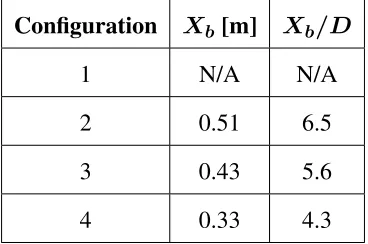
For this set of experiments, the bluff body was positioned at three different locations relative

to the wing. A diagram of the test section layout is shown in Fig. 2.3. Table 2.2 defines the three

bluff body positions tested.

+

-D = 0.076 m

Y X

X_b

(19)

Table 2.2Bluff body spatial configurations

Configuration Xb[m] Xb/D

1 N/A N/A

2 0.51 6.5

3 0.43 5.6

4 0.33 4.3

2.3 Wind Tunnel and Data Collection Methods

The pitch and heave kinematics are measured via a National Instruments NI PXIe-6363 I/O

module using a LabVIEW based data acquisition system with a nominal sampling rate of 50

kHz. Two U.S. Digital E6-10000 encoders with 0.07-degree resolution measure the wing’s

angular position while two Renishaw LM10 magnetic linear encoders with 0.03 mm resolution

measure the heave position. Aeroelastic experiments were conducted in the North Carolina

State University closed-return subsonic wind tunnel with a 0.81 m x 1.14 m x 1.17 m test

section. The freestream velocity for LCO experiments ranged from 6 m/s to 12 m/s, which

corresponds to an airfoil chord based Reynolds number range of 70×103 to 120×103. The

freestream windspeed (U∞) was monitored via a dynamic pressure transducer. For each test

case the wing was given initial deflections of 45 degrees, increasing the dynamic pressure in

increments of 0.1 psf until self-sustained oscillations began. Once LCO was established, the

wing was allowed to oscillate for one minute to avoid measuring transient behavior. Next, the

wing position data was recorded for two minutes and this process was repeated for increasing

(20)

Chapter

3

System Characterization

The aeroelastic apparatus is modeled as a coupled two degree-of-freedom mass-spring-damper

system. The equations of motion were derived previously by Kirschmeier et al. [10] and are

reproduced in equations (3.1) and (3.2).

m_Th¨+m_Wbx_θθ˙2sin(θ)−mWbxθθ¨cos(θ) +khh+chh˙+Ffsign(h˙) =CL 1 2ρU

2

∞cS (3.1)

I_θθ¨−mWbxθcos(θ)h¨+Mθ(θ) +cpθ˙+Mfsign(θ˙) =Cm 1 2ρU

2

∞c

2_S

(3.2)

Initial characterization of the effective stiffness in the pitch and heave degrees-of-freedom

were obtained via direct measurements from the ATI Gamma 6 axis load cell and Instron

4400R, respectively. The heave spring stiffness was measured to be constant over the range of

the range of heave deflections in the present experiments. The restoring moment response of the

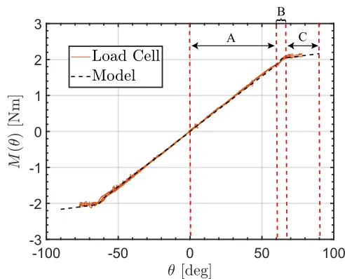
pitch DOF showed three distinct stiffness regions, labeled A, B, and C in Fig. 3.1. The transition

from region A to C is caused by one side of the pulley losing tension for large deflections,

reducing the effective stiffness by half. There are two transition angles marking the beginning

(21)

respectively and can be prescribed by fixing the amount of pre-tension in the pitch extension

springs. Wind-off free decay tests were also used to characterize the pitch nonlinearity. During

pitch-only and coupled pitch-heave free decay tests, a shift in the oscillation frequency was

observed at small pitch angles (≤6 deg). A power-law softening model was incorporated into

the piecewise stiffness model to capture this. Based on these observations, the form of the

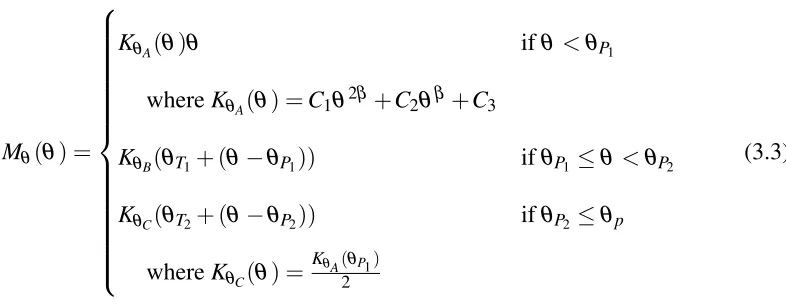
structural pitching moment equation is defined as:

M_θ(θ) =                               

K_θ_A(θ)θ ifθ <θP1

whereK_θ_A(θ) =C1θ2β +C2θβ+C3

K_θ_B(θT1+ (θ−θP1)) ifθP1≤θ <θP2

K_θ_C(θT2+ (θ−θP2)) ifθP2≤θp

whereK_θ_C(θ) =KθA(₂θP1)

(3.3)

whereθP1,2 are the transition angles andθT1,2are the modified transition angles which continuity

in the stiffness transition regions. The modified transition angles are defined as:

θT1 =

K_θ_A(θP1)θP1

K_θ_B ; (3.4)

θT2 =

K_θ_B(θT1+θP2−θP1)

K_θ_C ; (3.5)

Figure 3.1 shows the spring torque responses compared to the pitch stiffness model

de-scribed in Eq. 3.3. The piecewise model matches the experimental response well and captures

(22)

-100 -50 0 50 100 -3

-2 -1 0 1 2 3

A C

B{

Figure 3.1Spring torque measurements with load cell compared to Eqn. 3.3

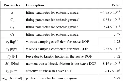
Appropriate values for the fitting terms in Eq. 3.3 as well as the stiffness and damping terms

in Eqs. 3.1 and 3.2 were obtained in MATLAB using the Delayed Rejection Adaptive

Metropo-lis (DRAM) Markov chain Monte Carlo (MCMC) algorithm as described by Kirschmeier et

(23)

Table 3.1Structural stiffness and damping properties

Parameter Description Value

β fitting parameter for softening model −4.35×10−1

C₁ fitting parameter for softening model 6.86×10−4

C₂ fitting parameter for softening model 9.74×10−2

C₃ fitting parameter for softening model 3.47

c_h[kg/s] viscous damping coefficient for heave DOF 1.73 cp[kg/s] viscous damping coefficient for pitch DOF 3.36×10−3 F_f [N] force due to kinetic friction in the heave DOF 1.02 M_f [Nm] moment due to kinetic friction in the heave DOF 8.19×10−3 k_h[N/m] effective stiffness in heave DOF 2.17×103

(24)

Chapter

4

Results and Discussion

4.1 LCO Response with Steady Inflow

The LCO response was first characterized without the presence of the upstream bluff body.

Figure 4.1(a) and 4.1(b) show the mean LCO amplitude vs windspeed for heave and pitch,

respectively. For each DOF, the mean amplitude is defined by taking the mean of the set of

(25)

6 7 8 9 10 11 12 0

0.1 0.2 0.3 0.4 0.5 0.6

(a)

6 7 8 9 10 11 12

45 50 55 60 65 70

(b)

Figure 4.1(a) Non-dimensional mean heave amplitude and (b) mean pitch amplitude vs windspeed for no-bluff-body case. Error bars represent one standard deviation.

From Fig. 4.1, it can be seen that the LCO amplitude increases with windspeed with small

error bars indicating nearly constant amplitude. Fig. 4.1(b) shows a distinct inflection point

which corresponds to the transition from the linear to the softening nonlinear pitch stiffness

regime. From Fig. 3.1 we see that this hardening transition region exists when the pitch

ampli-tude is between 60 and 65 degrees. Fig. 4.1(a) contains this inflection point as well, reflecting

the coupling between the two DOF. The trends seen in Fig. 4.1 are also reflected in the pitch

angle time histories (Fig. 4.2). Note that the trends in the pitch and heave responses are similar

and therefore, the remainder of the analysis in this paper will focus primarily on the response

(26)

0 15 30 45 60 -500

50

0 15 30 45 60

-500 50

0 15 30 45 60

-500 50

0 15 30 45 60

-500 50

0 15 30 45 60

-500 50

0 15 30 45 60

-500 50

0 15 30 45 60

-500 50

0 15 30 45 60

-500 50

Figure 4.2Pitch angle time histories for no-bluff-body case.

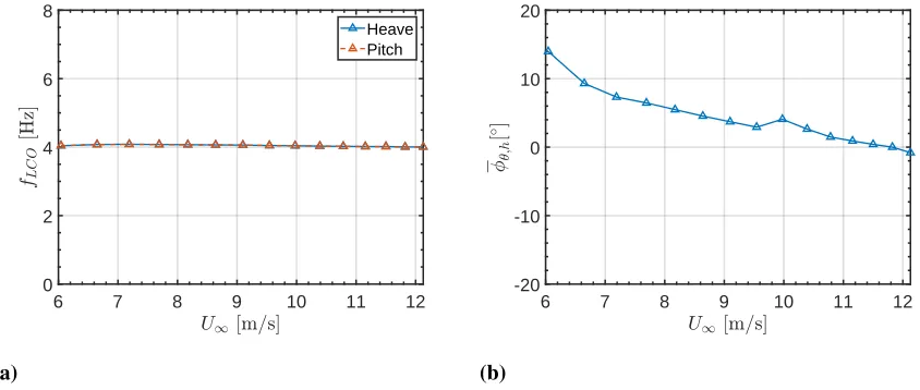
As shown in Fig. 4.3(a), the fundamental LCO frequency is approximately equal to 4 Hz

and is invariant with windspeed within 2%. The dominant frequency for each windspeed was

determined via FFT with a frequency resolution of∆f =1/N∆t=0.017Hz whereN∆t is the

total sampling time of 60 seconds. The frequency curves for the pitch and heave degrees of

freedom lie on top of each other which is characteristic of LCO initiated by a modal

conver-gence flutter instability. The average phase difference between pitch and heave position ( ¯φθ,h) was calculated using cross correlation and is shown in Fig. 4.3(b). We see that for this

(27)

6 7 8 9 10 11 12 0

2 4 6 8

Heave Pitch

(a)

6 7 8 9 10 11 12

-20 -10 0 10 20

(b)

Figure 4.3(a) Fundamental LCO frequency for pitch and heave vs windspeed and (b) mean pitch-heave phase difference ¯φθ,hvs windspeed for no-bluff-body case.

Exploring the frequency content of these responses via their power spectral densities (PSD)

(Fig. 4.4) reveals that in addition to the fundamental frequency peaks, there exist both even and

odd superharmonics which are characteristic of nonlinear oscillations. For increasing

(28)

0 5 10 15

9.1 10.0 10.8 11.5 12.1 Fundamental 2nd_Harmonic ₃rd_Harmonic

Figure 4.4Pitch angle PSD plotted vs windspeed for no-bluff-body case (PSD magnitude = arbitrary log scale)

4.2 LCO Response with Disturbed Inflow

4.2.1 Amplitude Modulation and LCO Superharmonic Frequency

Anal-ysis

It was shown previously that nonlinearities are introduced to the system through the pitch

stiff-ness (Eq. 3.3), nonlinear equations of motion (Eqs. 3.1, 3.2), and the aerodynamics. While the

system response in clean inflow conditions showed classical constant-amplitude LCO (Fig. 4.2),

nonlinearities can result in more complex dynamics when a system is introduced to external

disturbances. For example, a one DOF linear system exhibits a single resonance when the

forcing frequency matches the natural frequency of the system, while in a nonlinear system,

(29)

For the present system, the bluff body shedding frequency is close three times the

fun-damental LCO frequency. In order to investigate the effects of wing-wake frequency

interac-tion, the ratio f_shed/f_LCOis defined as the independent variable for each test case. Figure 4.5 presents pitch angle time histories, spanning the range of windspeeds tested, forX_b/D = 4.3. For windspeeds corresponding to f_shed/f_LCO ≤2.9, the deviation in LCO amplitude is rela-tively small compared to the mean amplitude. However, as the bluff body shedding frequency

migrates closer to 3f_LCO, the intensity of the amplitude modulation increases. As the wind-speed is increased further, the shedding frequency surpasses 3f_LCO and for f_shed/f_LCO>3.1, the modulation intensity diminishes again. This symmetry about f_shed/f_LCO=3 indicates that the bluff body shedding frequency, rather than the freestream windspeed, dominates the LCO

response in this regime.

0 50 100

-500 50

0 50 100

-500 50

0 50 100

-500 50

0 50 100

-500 50

0 50 100

-50 0 50

0 50 100

-50 0 50

0 50 100

-50 0 50

0 50 100

-50 0 50

Figure 4.5Pitch angle time histories forXb/D= 4.3 case.

The frequency content for a set of responses with the bluff body positioned atX_b/D=4.3 is provided in Fig. 4.6. Similar to the PSDs for the no-bluff-body case in Fig. 4.4, the peaks

(30)

addition of a peak corresponding to the bluff body shedding frequency. The shedding frequency

increases linearly from 9.5 Hz to 13.5 Hz with windspeed, following the expected trend for a

Strouhal number of 0.085 [18]. The shedding frequency that appears in the PSD also matches

the dominant frequency in the PSD of the bluff body load cell data. Additionally, there are two

sideband peaks which are symmetric about the fundamental frequency. These sidebands are

characteristic of amplitude-modulated signals and here, the frequency difference between the

fundamental frequency and one of the sideband peaks is equal to the modulation frequency.

0 5 10 15

9.1 10.0 10.8 11.5 12.1

f_shed 3rd_Harmonic

Fundamental 2nd_Harmonic

Figure 4.6Pitch angle PSD plotted vs windspeed forXb/D= 4.3 case (PSD magnitude = arbitrary log

scale)

4.2.2 Quantification of LCO Amplitude and Amplitude Modulation

In-tensity

Figure 4.5, qualitatively illustrates the system’s windspeed-dependent (and therefore shedding

(31)

distri-bution plots in which the set of peak pitch displacements, .i.e. the pitch amplitudes, for each

windspeed are overlaid. For the bluff body cases (Figs. 4.7(b), 4.7(c), 4.7(d)) there is an

addi-tional horizontal axis with the corresponding f_shed/f_LCO. Note that the darker shaded regions correspond to a tighter grouping of amplitudes while the lighter regions represent more

dis-perse amplitudes. Fig. 4.7(a) shows the no-bluff-body amplitude response in which the pitch

amplitude increases with windspeed with tight groupings indicating a constant pitch amplitude.

Figure 4.7(b), contains the pitch amplitudes for the case whereX_b/D=6.5. Here, the trend re-sembles Fig. 4.7(a) for sufficiently low values of f_shed/f_LCO; i.e., the mean amplitude increases with windspeed and the individual cycle amplitudes are tightly grouped. However, this trend is

interrupted as the bluff body shedding frequency nears 3f_LCO. For values of f_shed/f_LCO close to three, the dispersion in pitch amplitude increases significantly. A similar behavior is

exhib-ited by the case shown in Fig. 4.7(c) in which X_b/D= 5.6; however, here there is a stronger influence from the bluff body, causing the cycle amplitude to drop below 20 degrees at its

minimum. Figure 4.7(d), in which the bluff body is in the closest upstream position (Xb/D= 4.3), shows a significant disruption in the pitch amplitude trend with cycle amplitudes ranging

(32)

6 7 8 9 10 11 12 0 20 40 60 80 (a)

2 2.25 2.5 2.75 3 3.25 3.5

7 8 9 10 11 12

0 20 40 60 80 (b)

2.25 2.5 2.75 3 3.25

8 9 10 11 12

0 20 40 60 80 (c)

2.25 2.5 2.75 3 3.25

8 9 10 11 12

0 20 40 60 80 (d)

Figure 4.7Pitch amplitude distributions for (a) no-bluff-body, (b)Xb/D= 6.5, (c)Xb/D= 5.6, (d) Xb/D= 4.3.

In Fig. 4.8, the amplitude modulation intensity is quantified via the coefficient of variation

(CV) or the standard deviation of amplitude divided by the mean. The CV serves as a measure

of dispersion in LCO amplitude or how heavily the amplitude is modulated at a given point in

time. The local mean and standard deviation were obtained by dividing the time history into 10

second windows and interpolating to produce the contours seen in Fig. 4.8. Figure 4.8(a) shows

(33)

a non-modulated, steady LCO. For the bluff body cases, for windspeeds in which f_shed/f_LCO was not close to an integer value, the LCO exhibited a relatively small degree of amplitude

modulation, similar to the no-bluff-body case. However, as f_shedapproaches and passes through an integer multiple of fLCO, the system exhibits a drastic change in behavior. The system returns to a relatively low modulation intensity for f_shed/f_LCO ≥3.2, demonstrating the frequency-dominated nature of the phenomenon. This effect is reflected in Figure 4.8(b) which shows

two distinct bands of increased modulation intensity on either side of the f_shed/f_LCO=3 line. These regions of increased CV correspond directly to the regions of increased pitch amplitude

dispersion from Fig. 4.7(b). Similar behavior is exhibited in Figs. 4.8(c) and 4.8(d), however

with increased modulation intensity for decreasedX_b/D. The global maximum CV increased 300% between Figs. 4.8(b) and 4.8(c) and 530% between Figs. 4.8(b) and 4.8(d). Additionally,

(34)

(a) (b)

(c) (d)

Figure 4.8Pitch amplitude CV contours for (a) no-bluff-body, (b)Xb/D= 6.5, (c)Xb/D= 5.6, (d) Xb/D= 4.3.

4.2.3 Time-Frequency Analysis of LCO Modulation

Further characterization of the LCO amplitude modulation was performed via a via

time-frequency wavelet analysis of the LCO envelope. The envelope is defined as a spline

(35)

of the LCO envelope is shown as a series of scalograms which illustrate the evolution of the

modulation frequency over time.

Fig. 4.9 contains the CWTs and time histories corresponding to f_shed/f_LCO=2.8 for the three bluff body positions (a)X_b/D= 6.5, (b)X_b/D= 5.6, (c)X_b/D= 4.3. In this regime, where f_shed/f_LCO is sufficiently far from an integer value, the distance X_b/Dhas little influence on neither the modulation intensity nor the modulation frequency. The intensity of the modulation

for the three bluff body positions is uniform with respect to time and the dominant modulation

frequency is approximately 0.9 Hz. By examining the PSD of the pitch angle time history

for X_b/D = 4.3 (Fig. 4.6), we see that the LCO third harmonic frequency is 12.2 Hz and the shedding frequency is equal to 11.3 Hz. The difference between these two frequencies (f_shed−

3fLCO) is equal to the modulation frequency found in Fig. 4.9(c), indicating behavior analogous to a beat phenomenon except that the interaction is with a harmonic frequency rather than the

fundamental. Extending the same analysis to the other configurations (Figs. 4.9(a) and 4.9(b)),

the modulating frequency is equal to f_shed−3f_LCOin both cases.

(a) (b) (c)

(36)

Fig. 4.10 contains envelope CWTs and pitch angle time history plots for f_shed/f_LCO=2.9. Figure 4.10(a) shows an amplitude modulation that is relatively uniform in intensity and

fre-quency with a dominant modulation frefre-quency equal to f_shed−3f_LCO. Compared to Fig. 4.9(a), the modulation is lower in frequency due to the smaller difference between 3fLCO and fshed. When the bluff body is moved toX_b/D= 5.6 (Fig. 4.10(b)), f_shed−3f_LCOis still present in the envelope CWT, however it is no longer the only modulation frequency. In this case, the LCO

response alternates between two modulation modes, represented by the two dominant

modula-tion frequencies seen in the envelope CWT. Further evidence of this is provided by Fig. 4.10(c)

in which X_b/D= 4.3 and the two modes are even more pronounced. Among the two distinct modulation modes present, the first is a low frequency mode that persists during the first 60

seconds of the trial and causes a relatively intense modulation of the LCO amplitude. The

sec-ond is a higher frequency mode representing f_shed−3f_LCO which dominates between t =80 sec. andt =120 sec. and produces a less intense modulation. Figure 4.10(c) also shows

tran-sient period between the two modes (t =60 sec. to t =80 sec.) in which neither frequency

dominates entirely.

(a) (b) (c)

(37)

The pitch angle time histories and envelope CWTs for f_shed/f_LCO = 3.1 are shown in Fig. 4.11. Here, the system exhibits responses similar to the case in Fig. 4.10 where f_shed/f_LCO= 2.9. The amplitude modulation is uniform in frequency and intensity for X_b/D = 6.5 with a dominant modulation frequency equal to f_shed−3fLCO(Fig. 4.11(a)). For the case ofXb/D= 5.6, the modulation becomes less uniform, with lower frequency content appearing sporadically

throughout the time history (Fig. 4.11(b)). For the case ofX_b/D= 4.3, the low frequency modu-lation dominates the signal along with the f_shed−3f_LCO(Fig. 4.11(c)). Referencing Fig. 4.7(d), it is clear that the cause of the large amplitude dispersion corresponds due to the lower

fre-quency mode. Comparing Fig. 4.11(c) to Fig. 4.10(c), the switching between the two primary

modulation modes does not occur over a consistent period, as evidenced by a more rapid

alter-nation between modes seen in Fig. 4.11(c).

(a) (b) (c)

Figure 4.11Time-frequency content of pitch angle envelope (bottom) with corresponding pitch angle time history (top) for (a)Xb/D= 6.5, (b)Xb/D= 5.6, and (c)Xb/D= 4.3 where fshed/fLCO=3.1.

(38)

modulation. Figures 4.9 and 4.12 both show a low intensity modulation with a dominant

mod-ulation frequency equal to f_shed−3f_LCO, that is invariant with respect to bluff body position.

(a) (b) (c)

Figure 4.12Time-frequency content of pitch angle envelope (bottom) with corresponding pitch angle time history (top) for (a)Xb/D= 6.5, (b)Xb/D= 5.6, and (c)Xb/D= 4.3 where fshed/fLCO=3.25.

4.2.4 Instantaneous Phase and Aeroelastic Energy Analysis

The efficiency of aeroelastic systems is often discussed in literature in the context of energy

har-vesting and bio-inspired vehicle locomotion. Several studies that have examined the efficiency

of pitch-heave aeroelastic systems have concluded that the phase angle difference between the

two degrees of freedom is an important parameter for predicting efficiency. Anderson et al. [1]

conducted an experiment in which the propulsive efficiency of an airfoil undergoing prescribed

motion was determined as a function of the phase angle between heave and pitch. They found

the optimal phase angle for propulsion to be about 75 degrees since this condition produces

favorable timing of the leading edge vortex (LEV) shedding, facilitating the formation of a

thrust-producing reverse Kármán street. Similarly, McKinney and DeLaurier [15] found that

a phase angle of about 90 degrees is optimally efficient for power extraction in a

(39)

to the total power available in the oncoming flow passing through the swept area normal to

the mean wind vector. Later, Kinsey and Dumas [9] showed that LEV shedding is an

impor-tant mechanism by which favorable synchronization is achieved between the lift force and the

heaving velocity, thus controlling the power input to the system.

In order to examine the influence of the bluff body in this context, we begin by performing

a phase plane analysis of the LCO. Figure 4.13 contains the pitch-heave displacement phase

portraits for (a) no-bluff-body (U∞=10.4m/s) and (b)Xb/D = 6.5, (c) Xb/D= 5.6, and (d) X_b/D= 4.3 for similar windspeed (f_shed/f_LCO=2.9). In Fig. 4.13(a), the no-bluff-body motion trajectory maintains little deviation from the closed orbit defined by the thin ellipse. This is in

contrast to the trajectories for the three bluff body cases (Figs. 4.13(b), 4.13(c), 4.13(d)) in

(40)

-0.5 -0.25 0 0.25 0.5 -100 -50 0 50 100 (a)

-0.5 -0.25 0 0.25 0.5 -100 -50 0 50 100 (b)

-0.5 -0.25 0 0.25 0.5 -100 -50 0 50 100 (c)

-0.5 -0.25 0 0.25 0.5 -100 -50 0 50 100 (d)

Figure 4.13Phase portraits for (a) no-bluff-body (U∞=10.4m/s) and (b)Xb/D= 6.5, (c)Xb/D= 5.6,

and (d)Xb/D= 4.3 (fshed/fLCO=2.9).

Since the phase portraits shown in Fig. 4.13 contain the entire time history of the LCO,

it is difficult to gain a detailed understanding of how the phase space trajectory evolves with

time. To determine the phase angle difference as a function of time, the instantaneous

pitch-heave phase difference,φθ,h, was calculated as a function of time via the discrete-time analytic signal which is a complex-valued function comprised of the real-valued LCO signal and its

(41)

is described by Marple [14]. The form of the analytic signal is:

z(t) =z_r(t) +iz_i(t) =x(t) +HT[x(t)] (4.1)

wherez_r(t)is the real component ofz(t), z_i(t)is the imaginary component ofz(t),x(t)is the original signal andHT[]is the Hilbert transform operation. Next, the instantaneous phase angle

is computed as follows:

φ(t) =arctan

z_i(t)

z_r(t) (4.2)

whereφ(t)is the instantaneous phase angle. For this system, the instantaneous phase difference

between pitch and heave is calculated as the differenceφ_θ,h=φ(t)pitch−φ(t)heave.

Fig. 4.14 showsφ_θ,hfor the same four configurations displayed in Fig. 4.13. Figure 4.14(a) demonstrates that the instantaneous phase differenceφθ,his constant within 1.5 degrees in the absence of an upstream bluff body. Figs. 4.14(b), 4.14(c), and 4.14(d) show significant

modu-lation ofφθ,hthat occurs as the wing oscillates through the bluff body wake. The modulation ofφθ,hcreates a path through the phase space that is time-dependent when the bluff body is up-stream. This is qualitatively reflected by the phase portraits in Fig. 4.13. Note that the frequency

of theφ_θ,hmodulation is dependent on the bluff body spatial configuration. For the case where X_b/D=6.5 (Fig. 4.14(b)), the phase difference oscillates at a frequency equal to f_shed−3f_LCO for all time shown. For both theX_b/D=5.6 andX_b/D=4.3, (Figs. 4.14(c) and 4.14(d), respec-tively) the frequency of phase modulation is not uniform with time. Comparing the frequency

of the phase modulation in both cases to their respective amplitude modulation frequencies

(Figs. 4.10(b)) and 4.10(c)), we find that they are equal. Also, note that the time periods of

intenseφθ,hmodulation (t=0 sec tot=60 sec) seen in Fig. 4.14(d) correspond directly to the time periods of intense amplitude modulation seen in Fig. 4.10(c). Conversely, the time period

(42)

intensity amplitude modulation, indicating a correlation between the magnitude of the phase

differenceφθ,hand the LCO amplitude.

0 10 20 30 40 50 60

-60 -40 -20 0 20 40 60 -50 0 50 (a)

0 20 40 60 80 100 120

-60 -40 -20 0 20 40 60 -50 0 50 (b)

0 20 40 60 80 100 120

-60 -40 -20 0 20 40 60 -50 0 50 (c)

0 20 40 60 80 100 120

-60 -40 -20 0 20 40 60 -50 0 50 (d)

Figure 4.14θ(top) andφθ,h(bottom) vs time for (a) no-bluff-body (U∞=10.4m/s) and (b)Xb/D=

6.5, (c)Xb/D= 5.6, and (d)Xb/D= 4.3 (fshed/fLCO=2.9).

A phase portrait is shown in Fig. 4.15, depicting the phase relationship between φ_θ,h and the LCO amplitude. The orange trajectory represents the no-bluff-body configuration from

(43)

(θA) with time. The blue curve represents theXb/D=6.5 case from Fig. 4.14(b) and shows a strong correlation betweenφθ,h andθA. The phase portrait maintains an elliptical shape, with the arrow indicating the direction of time. When read in the counterclockwise direction, this

plot shows thatφ_θ,hleadsθAby approximately 90 degrees.

-30 -20 -10 0 10 20 30

45 50 55 60 65 70 75 80

Figure 4.15Phase portrait ofθAvsφθ,hfor no-bluff-body (U∞ = 10.4m/s) andXb/D= 6.5

(fshed/fLCO=2.9).

The previously mentioned studies [1, 15, 9] focused primarily on the wing efficiency for

the purposes of exploiting the dynamics to extract power from the structure. However, since

the aeroelastic system in the present study is not designed for energy harvesting, any net power

into the structure manifests as a change in the kinematics. For the case of a constant amplitude

aeroelastic LCO, the net aerodynamic work is balanced by the losses due to structural damping

forces over a given cycle. Thus, it follows that the average net power over a cycle is equal to

(44)

positive or negative, where the amplitude will grow or decay, respectively. For the present

system, the available power is considered to be constant for a fixed freestream windspeed

and the bluff body alters the distribution of kinetic energy in the flowfield. Therefore, any net

power into the structure must be due to a change in aeroelastic efficiency. We define the total

mechanical energy of the aeroelastic system,E, as the sum of the kinetic and potential energy,

T+U. From this definition, the net work done on the structure (Wnet) includes contributions from the aerodynamics (WA) and the structural damping (WD) and is defined as:

Wnet =WA−WD=T+U−E0 (4.3)

whereE₀ is the initial energy of the wing at thet=0 reference point for the aerodynamic and

damping work. This definition can be expanded by incorporating the definitions forT andU

for this system, previously derived by Kirschmeier et al. [11]:

W_net =1 2mT

˙ h2+1

2Iθ ˙

θ2−mWbxθh˙θ˙cosθ+ 1 2Khh

2₊Z θ 0

M_θ(θ)dθ−E0 (4.4)

where M_θ(θ) is the function defining the pitch nonlinearity (Eq.3.3). Next, the net

instanta-neous power is calculated as the numerical time derivative of work via a central difference

scheme:

Pnet(ti)≈

W_net(t_i+∆t)−W_net(t_i−∆t)

2∆t (4.5)

where ∆t is the sampling period. Since we are interested in power on the time scale of the

(45)

calculated by applying a central moving average to the instantaneous power:

¯

P_net(t_i) = 1 N

1 2(N−1)

∑

j=−1

2(N−1)

P_net(t_i₊_j) (4.6)

where N is size of the sliding window which is set to cover a single wing cycle period (0.25

sec via PSD) andt_iis theith data point.

Figure 4.16(a) showsφθ,hand ¯Pnetas functions of time for theXb/D=6.5, fshed/fLCO=2.9 case. We see that ¯Pnet oscillates at the same frequency as bothφθ,h and the LCO amplitude. Also,φ_θ,hand ¯Pnet are in phase with each other; i.e., maximumφθ,hcorresponds to maximum

¯

P_net. Note that this is in contrast to Fig. 4.15 whereφ_θ,hleadsθA by approximately 90 degrees. This result makes sense when we consider that ¯P_net is the time derivative of the average total energy, ¯E. That is, maximum and minimumφθ,hcorrespond to the maximum rates of amplitude increase and decrease, respectively, as seen in (Fig. 4.16(b)).

70 75 80 85 90 95 100

-30 -20 -10 0 10 20 30 -4 -2 0 2 4 0

70 75 80 85 90 95 100 -50 0 50 Maximum energy loss Maximum energy gain

(46)

Chapter

5

Conclusion

5.1 Conclusion

The aim of this research is to elucidate the complex interactions between a nonlinear aeroelastic

wing and an oscillating wake shed from an upstream bluff body. The main conclusions stem

from the characterization of LCO amplitude modulation and can be summarized as follows:

1. The cases in which the bluff body was present showed amplitude-modulated responses in

both the pitch and heave degrees of freedom. The intensity of this modulation, defined by

the coefficient of variation of the amplitude, increases sharply as the difference between

the LCO third harmonic and the bluff body shedding frequency decreases. It is possible

that similar interaction exists for shedding frequency regimes near integer multiples other

than three, thus indicating the potential for future work in further exploration of the

system dynamics.

2. The streamwise distance between the bluff body and the wing influenced the intensity

(47)

and increased the variation of the modulation intensity itself with time. The greater

in-fluence from the bluff body at closer distances is attributed to increased strength of the

impinging wake vortices.

3. The modulation frequency was equal to f_shed−3f_LCO for the X_b/D=6.5 case for all frequency ratios f_shed/f_LCO. This was true for all bluff body spatial configurations when f_shed/f_LCO≤2.8 or f_shed/f_LCO≥3.2. However, when 2.8≤ f_shed/f_LCO≤3.2, decreas-ingX_b/D was shown to cause intermittent alternation between two modulation modes, each with distinct characteristic intensity and frequency.

4. The mechanism of amplitude modulation was revealed through instantaneous phase and

energy analysis. The presence of the bluff body alters the dynamics such that

instanta-neous pitch-heave phase difference modulates with time. This phase difference manifests

as an effective change in the aeroelastic efficiency of the wing. That is, for a limit cycle

to maintain constant amplitude, the phase difference between pitch and heave must be

such that the average power over a cycle is zero. When the bluff body alters this phase

difference, the balance of power into and out of the structure over a cycle is disrupted,

(48)

REFERENCES

[1] J. M. Anderson, K. Streitlien, D. S. Barrett, and M. S. Triantafyllou. Oscillating foils of high propulsive efficiency. Journal of Fluid Mechanics, 360:S0022112097008392, apr 1998.

[2] William Blake and Dieter Multhopp. Design, performance and modeling considerations for close formation flight. In23rd Atmospheric Flight Mechanics Conference, Reston, Virigina, aug 1998. American Institute of Aeronautics and Astronautics.

[3] A W Bloy, M G West, K A Lea, and M Joiima’a$. Lateral aerodynamic interference between tanker and receiver in air-to-air refueling. Journal of Aircraft, 30(5):705–710, sep 1993.

[4] Jerry M Chen and Chih-Chung Choa. Freestream Disturbance Effects on an Airfoil Pitch-ing at Constant Rate. Journal of Aircraft, 36(3):507–514, may 1999.

[5] J.F. Derakhshandeh, M. Arjomandi, B. Dally, and B. Cazzolato. Flow-induced vibration of an elastically mounted airfoil under the influence of the wake of a circular cylinder.

Experimental Thermal and Fluid Science, 74:58–72, jun 2016.

[6] Earl H Dowell and Deman Tang. Nonlinear Aeroelasticity and Unsteady Aerodynamics.

AIAA Journal, 40(9):1697–1707, sep 2002.

[7] L. Gammaitoni, F. Marchesoni, E. Menichella-Saetta, and S. Santucci. Intermittency in nonlinear stochastic systems. Physics Letters A, 156(1-2):37–41, jun 1991.

[8] Philip W. Hammer, Nathan Platt, Stephen M Hammel, James F Heagy, and Bryan D Lee. Experimental Observation of On-Off Intermittency.Physical Review Letters, 73(8):1095– 1098, aug 1994.

[9] T Kinsey and G Dumas. Parametric Study of an Oscillating Airfoil in a Power-Extraction Regime. AIAA Journal, 46(6):1318–1330, jun 2008.

[10] B. Kirschmeier and M. Bryant. Toward efficient aeroelastic energy harvesting through limit cycle shaping. InActive and Passive Smart Structures and Integrated Systems 2016, volume 9799. SPIE, apr 2016.

[11] B. Kirschmeier, G. Pash, Z. Gianikos, and M. Bryant. Aeroelastic Inverse: Estimation of aerodynamic loads during dynamic stall flutter. In Submission: Journal of Fluids and

(49)

[12] Benjamin Kirschmeier and Matthew Bryant. Experimental investigation of wake-induced aeroelastic limit cycle oscillations in tandem wings. Journal of Fluids and Structures, 81:309–324, aug 2018.

[13] D. Lentink, F. T. Muijres, F. J. Donker-Duyvis, and J. L. van Leeuwen. Vortex-wake interactions of a flapping foil that models animal swimming and flight. Journal of

Exper-imental Biology, 211(2):267–273, jan 2008.

[14] L. Marple. Computing the discrete-time "analytic" signal via FFT. IEEE Transactions on

Signal Processing, 47(9):2600–2603, 1999.

[15] William McKinney and James DeLaurier. Wingmill: An Oscillating-Wing Windmill.

Journal of Energy, 5(2):109–115, mar 1981.

[16] Leonard Meirovitch. Fundamentals of Vibrations. Waveland Pr Inc., jul 2010.

[17] Brandon E Merrill and Yulia T Peet. Effect of Impinging Wake Turbulence on the Dy-namic Stall of a Pitching Airfoil. AIAA Journal, 55(12):4094–4112, dec 2017.

[18] Atsushi Okajima. Strouhal numbers of rectangular cylinders.Journal of Fluid Mechanics, 123:379–398, 1982.

[19] D Poirel, Y Harris, and A Benaissa. Self-sustained aeroelastic oscillations of a NACA0012 airfoil at low-to-moderate Reynolds numbers. Journal of Fluids and

Struc-tures, 24(5):700–719, jul 2008.

[20] Dominique C Poirel and Stuart J Price. Structurally Nonlinear Fluttering Airfoil in Tur-bulent Flow. AIAA Journal, 39(10):1960–1968, oct 2001.

[21] Knut Streitlien, George S Triantafyllou, and Michael S Triantafyllou. Efficient foil propulsion through vortex control. AIAA Journal, 34(11):2315–2319, nov 1996.

[22] Thomas W Strganac, Jeonghwan Ko, and David E Thompson. Identification and Control of Limit Cycle Oscillations in Aeroelastic Systems. Journal of Guidance, Control, and

Dynamics, 23(6):1127–1133, nov 2000.

[23] Y. T. Tsui. On Wake-Induced Flutter of a Circular Cylinder in the Wake of Another.

Journal of Applied Mechanics, 44(2):194, feb 1977.

(50)

[25] Miguel R. Visbal and Daniel J. Garmann. Numerical Investigation of Spanwise End Effects on Dynamic Stall of a Pitching NACA 0012 Wing. In 55th AIAA Aerospace

Sciences Meeting, Reston, Virginia, jan 2017. American Institute of Aeronautics and

As-tronautics.

[26] Rafal ˙Zbikowski. On aerodynamic modelling of an insect–like flapping wing in hover for micro air vehicles. Philosophical Transactions of the Royal Society of London. Series A: