Through Wall Detection with Relevance Vector Machine
Fang-Fang Wang*, Ye-Rong Zhang, Hua-Mei Zhang, Lin Hai, and Gong Chen
Abstract—In this paper, through-wall detection problem using a data-driven model is addressed. The original problem is cast into a regression one and successively solved by means of the relevance vector machine (RVM). Multiple scattering is included in the nonlinear relationship between the feature vector extracted from the backscattered field and the position of the target obtained through a training phase using RVM; hence the nonlinearity inherent in the problem is considered. Besides, the presence of the wall is also contained in this relationship. The predictions obtained by RVM are probabilistic which capture uncertainty, and we can define error-bars for the predicted results. Therefore, the ill-posed nature of the problem is accounted for naturally, rather than using other regularization schemes. To access the effectiveness, accuracy and robustness of the proposed approach, numerical results related to a two-dimensional geometry are presented. This method is demonstrated efficient qualitatively and quantitatively.
1. INTRODUCTION
In recent years, sensing through obstacles such as walls, doors, and other visually opaque materials using microwave signals has emerged as a powerful tool supporting a range of civilian and military applications. It is of practical importance to detect, locate, characterize and imaging an object with electromagnetic waves in wide areas such as subsurface sensing, biomedical imaging and through-wall imaging (TWI) [1]. TWI has recently sought out for surveillance and reconnaissance in urban environment, which can be employed to detect and locate survivors for succors in search and rescue in natural disasters, such as earthquakes and avalanches [2, 3].
Research activities related to imaging of stationary target behind walls can be grouped into four main topics: electromagnetic (EM) modeling for wave propagation and scattering from building interiors and targets therein; mitigation of wall returns; data processing approaches (i.e., imaging algorithms); new configuration based on multi-array observation [4]. In this paper, we are concerned with the data processing approaches. Generally, TWI problem has been approached in two ways: some employed synthetic aperture radar (SAR) processing methods and appropriately modified them in order to account for the presence of walls [5–7]; others cast the original problem into an inverse scattering one governed by wave equations [8, 9]. Specially, lots of EM inversion techniques have been proposed to address the problem of inverse scattering, mostly based on the discretization of the scattering integral equation or on iterative minimization procedures [10–12].
All of the imaging approaches mentioned above for TWI problem is based on physical modeling. However, the lack of required data and the expense of data acquisition can limit the practical application of physics-based models. To overcome these limitations, researchers have used data-driven models as an alternative, or a complement, to physics-based models for TWI problem [13–15]. Examples of such models include artificial neural network (ANN), support vector machine (SVM), and relevance vector machine (RVM). They are characterized by their ability to capture the underlying physics of the system
Received 5 May 2015, Accepted 13 June 2015, Scheduled 25 June 2015 * Corresponding author: Fang-Fang Wang (wangff@njupt.edu.cn).
simply by examination of the inputs and outputs of the system. Taking advantage of data-driven model, the TWI problem is reformulated as a regression one, where the data (i.e., scatter-field measurement) and the unknowns (i.e., the position of the object) are related by means of an approximated function to be estimated through an off-line data fitting process. In this way, the effects caused by walls can be included in the mapping obtained after the training phase. Therefore, this technology is not sensitive to a priori knowledge on the wall or the room geometry.
In this paper, RVM is applied in TWI for target detection. It is well known that TWI problem is nonlinear and ill-posed. Fortunately, RVM is a nonlinear sparse machine learning algorithm, and with Bayesian inference, it has better generalization than SVM [16]. Besides, RVM employs the identical function form to SVM, but compared with SVM, RVM has the superiorities of supplying probabilistic output information, fixed hyper-parameters and easy realization. Moreover, rather than utilizing regularization to address the ill-posed characteristic of the TWI problem, a statistical prior is imposed on the weights to be estimated. Using RVM, the ill-posed nature of the TWI problem is accounted for naturally, since the goal is not to find a single estimation of the weights, but rather the Bayesian analysis estimates a full-posterior density function on the weights (naturally accounting for uncertainties caused by the ill-posed nature of the problem).
The remainder of this paper is organized as follows. In Section 2, we provided a description of the TWI problem. Then, an introduction of RVM is given in Section 3. The simulation results are presented in Section 4. Finally, some conclusions and final remarks are provided.
2. PROBLEM DESCRIPTION
The actual geometry of the problem is depicted in Fig. 1. The scatterer is hidden behind a known structure resembling the walls of a room. The walls have relative dielectric permittivity εr, and
conductivity σ. The medium inside and outside the wall structure is assumed as free space whose dielectric permittivity is denoted asε0. The magnetic permeability everywhere is the one of free space
μ0. The investigation domain D is illuminated by the transmitting antenna (TX). The scattered field
is collected by the receiving antenna (RX), which then moves in order to synthesize a measurement line
L. The space between two consecutive observation locations is d.
TWI problem can be recast into an inverse scattering one which aims at determining both the geometric and physical properties of the scattering objects from knowledge of the measured field due to the illumination of the incident electromagnetic wave. The inverse scattering problem is then reformulated as a regression one where the unknowns (i.e., the position as well as the geometric and dielectric characteristic of the target) are directly evaluated from the data (i.e., the value of the scattered field) by approximating the data-unknowns relation through an off-line data fitting process. The relationship between the information of the backscattered fields and target’s properties is generalized
to a nonlinear function
y=f(x) (1)
Here, y represents one of the target’s properties such as position for through-wall detection, and x is a vector containing features extracted from the collected scattering fields such as a set of amplitude of the target’s scattered field at each observation location.
3. RELEVANCE VECTOR MACHINE
The structure of the RVM is described by the sum of product of weights and kernel functions. It makes prediction based on a function of the form
y(x;w) =
N
n=1
wnK(x,xn) +w0 =φT(x)w (2)
where w= [w0, . . . , wN]T and φ(x) = [1, K(x,x1), K(x,x2), . . . , K(x,xN)]T are vectors, and N is the
number of samples in training dataset. The kernel function K(·,·) corresponds to an inner product of vectors in the higher dimensional feature space. The basic kernel functions are as follows:
Linear: K(xi,xj) =xTi xj.
Polynomial: K(xi,xj) = (γxTi xj+r)d.
Gaussian radial basis function: K(xi,xj) = exp(−γxi−xj2). Sigmoid: K(xi,xj) = tanh(γxTi xj +r).
Here,γ,r and dare kernel parameters.
Given a set of input vectors{xn}Nn=1along with corresponding output scalars{tn}Nn=1, and assuming
that the outputs are independent and contaminated with mean-zero Gaussian noiseεnwith varianceσ2
tn=y(xn;w) +εn (3)
The likelihood of the dataset can be written as
pt|w, σ2= (2πσ2)−N/2exp
− 1
2σ2 t−Φw 2
(4)
where target vectort= [t1, . . . , tN]T,Φis theN×(N+ 1) design matrix withΦ= [φ(x1), . . . , φ(xN)]T.
Maximum-likelihood estimation ofwandσ2 from (4) will generally lead to severe over-fitting. To avoid this, a zero-mean Gaussian prior distribution over wwith variance α−1 is added as
p(w|α) =
N
i=0
Nwi|0, α−i 1
(5)
where hyper-parameter vector isα= [α0, . . . , αN]T. This introduction of an individual hyper-parameter
for every weight is the key feature of the model and is ultimately responsible for its sparsity properties. The posterior distribution over the weight is then obtained from Bayes rule:
pw|t,α, σ2= p
t|w, σ2p(w|α)
p(t|α, σ2) = (2π)−
(N+1)/2|Σ|−1/2
exp
−1
2(w−μ)
T Σ−1(w−μ) (6)
where the posterior mean vector μand covariance matrixΣare as follows:
μ = σ−2ΣΦTt (7)
Σ = σ−2ΦTΦ+A−1 (8)
with matrix A= diag(α0, α1, . . . , αN).
The likelihood distribution over the training targets can be marginalized with respect to the weights to obtain the marginal likelihood, which is also a Gaussian distribution
pt|α, σ2=
pt|w, σ2p(w|α)dw= (2π)−N2 |C|−12 exp
−1
2t
TC−1t
with covariance matrix C=σ2I+ΦA−1ΦT.
Values ofα and σ2 that maximize the marginal likelihood can not be obtained in closed form, and
an iterative re-estimation method is required. The following approach gives:
αnewi = γi
μ2 i
(10)
σ2new = t−Σμ
2
N−iγi
(11)
with μi is the ith posterior mean weight (7) and the quantities γi = 1−αiΣii with the ith diagonal
element Σii of the posterior weight covariance (8).
In the iterative maximization of marginal likelihood, many of hyper-parametersαi tend to infinity,
yielding a posterior distribution (6) of the corresponding weight wi that tends to be a delta function
centered around zero. The corresponding weight is thus deleted from the model, along with its associated basis function. The remaining examples with nonzero associated weight are called the relevance vectors. Given an input vector x∗, the probability distribution of the corresponding output is given by the predictive distribution
py∗|x∗,αˆ,σˆ2=
py∗|x∗,w,σˆ2pw|y,αˆ,σˆ2dw (12)
which has a Gaussian form,p(y∗|x∗,w,σˆ2) =N(y∗, σ∗2), where the mean and variance of the prediction are,
y∗ = φT(x∗)μ (13)
σ∗2 = ˆσ2+φT(x∗)Σφ(x∗) (14)
respectively. ˆα and ˆσ2 are the estimation of the hyper-parameter vectorα and of the noise σ2.
4. SIMULATION RESULTS
To validate this through-wall detection method experimentally based on RVM, firstly, we conduct numerical experiments using finite-difference time-domain (FDTD) to collect backscattered field from the target at each observation location of receiving antenna. The numerical simulator FDTD consists in discretizing the Maxwell’s equations in both space and time to obtain an approximate solution directly in the time domain through an iterative process.
In our simulation, a metallic circular cylinder resided in a room is taken into account as shown in Fig. 1. The thickness of walls is 0.2 m. The investigation domain isD= [−1.08,1.08]×[0.25,3.64] m2.
The conductivityσ and relative permittivityεr of the walls are set as a standard value of 0.01 S/m and
8, respectively. The geometry of the room is discretized with the FDTD square cells of 1 cm length. The time resolution is 19.25×10⁻¹²s. The transmitting antenna (TX) is fixed in the position of (0, 0) which is 0.05 m away from the front wall. To model the EM illumination of the modeled room and objects in it with an UWB short pulse, the transmitter dipole antenna is fed by a 4.5 ns Gaussian pulse modulated by a 0.5 GHz sine wave. The receiving antenna (RX) is 0.04 m away from the same side of the wall, which moves and synthesizes a measurement apertureL= 2.4 m. At each observation point, the scattered field introduced by the scatterer is obtained by subtracting, from the total electric field computed in the presence of the scatterer, the electric field computed in the absence of the scatterer.
Once obtaining the scattered field from the target, some features can be extracted from these fields. In this paper, we consider amplitude of the scattered field at individual observation location as the feature. Ultimately, a vector containing these features is fed into RVM predictor as an input and the position of the scatterer is the output.
The RVM must be trained by exploiting some input-output patterns suitably chosen so as to give an exhaustive representation of the through-wall detection problem being investigated. To do this, the training dataset is achieved by repeated simulations varying the position of the target as follows:
xn=−1.13 +nΔx, n= 0,1, . . . , Δx= 0.1 m yn= 0.2 +nΔy, n= 0,1, . . . , Δy= 0.1 m
In the same way, for testing samples, the positions of the target are made to vary in such way:
xn=−1.1 +nΔx, n= 0,1, . . . , Δx= 0.1 m yn= 0.25 +nΔy, n= 0,1, . . . , Δy= 0.1 m
(16)
In RVM regression, the kernel function is selected as the Gaussian kernel, which is given by
K(xi,xj) = exp
−γxi−xj2
(17)
whereγ is the variance of the kernel function which is tuned using cross-validation in the training phase. Since the assessment is focused on the target detection through a wall, the degree of match between the actual and predicted position comprised of horizon and depth is firstly evaluated qualitatively. The results are shown in Fig. 2. The figure shows good performance of the RVM predictor.
In most circumstance, the predicted value for x-coordinate or y-coordinate of the target center matches the actual value pretty well. However, for some position away from the transmitting antenna,
-1.5 -1 -0.5 0 0.5 1 1.5
-1.5 -1 -0.5 0 0.5 1 1.5
Actual Horizon, m
Predicted Horizon, m
0 0.5 1 1.5 2 2.5 3 3.5 4
0 0.5 1 1.5 2 2.5 3 3.5 4 4.5
Actual Depth, m
Predicted Depth, m
(a) (b)
Figure 2. Predicted values of (a) x-coordinate and (b) y-coordinate of the target center versus the actual ones.
0 20 40 60 80 100
-0.6 -0.5 -0.4 -0.3 -0.2 -0.1 0 0.1 0.2 0.3
Index
Errors of Horizon, m
-0.6 -0.4 -0.2 0 0.2 0.4 0.6 0.8
Errors of Depth, m
(a) (b)
0 20 40 60 80 100
Index
there are some big errors in the predicted results. Since the transmitting antenna is fixed in the position of (0, 0), when the target is far from the transmitter, the electromagnetic wave arriving at the target is negligible because of the attenuation of the propagation.
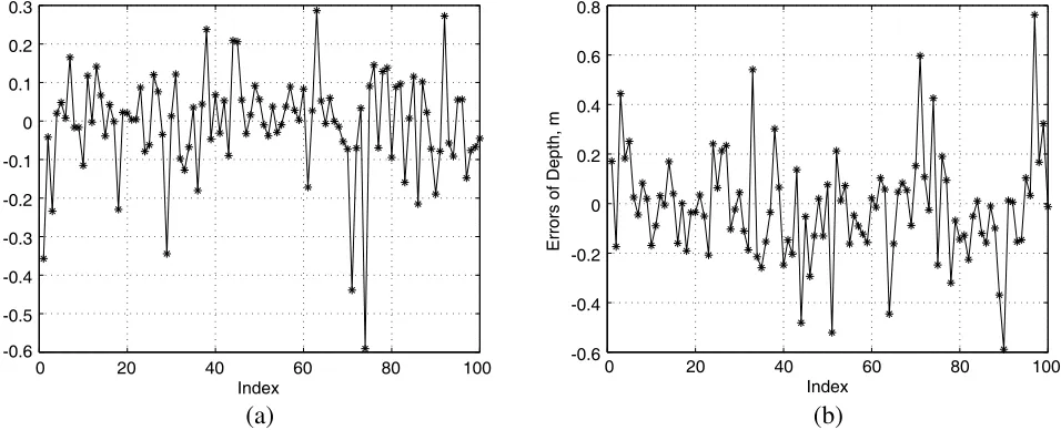
For 100 samples in testing dataset, the difference between the actual and predicted values for horizon and depth of the target is illustrated in Figs. 3(a) and (b), respectively. Minority of the samples present a big error. Generally, most of the errors are under 0.2 m.
In order to estimate the effectiveness and accuracy of the RVM predictor for through-wall target detection quantitatively, let us define the relative error of the prediction for the position, i.e., x -coordinate andy-coordinate:
ςx = |xact−l xpre|
x , ςy
= |yact−ypre|
ly
(18)
Here the variables with subscript act stand for the actual values and those with subscript pre for the predicted ones. lx, ly denote the total horizontal value and depth of room, respectively. In the
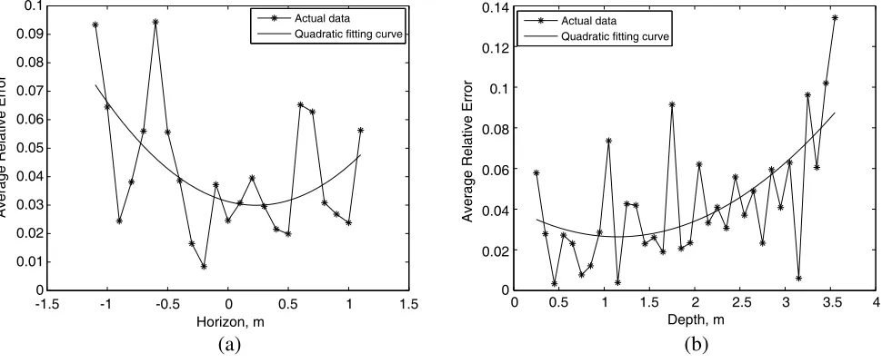
RVM-based approach for TWI problem, the estimation function relating the backscattered field and the target’s information such as positions is based on the training dataset in which the positions of the target are simulated within the room. In that case, the predicted positions of the target are also within the room. Fig. 4 shows the average relative error for different horizontal values and depths. The relative errors for horizon of the target do not exceed 0.1, and the minimal relative error is about 0.01. When the depth of the target is small, the relative error is small. The relative error almost grows with the value of the depth. Thus, the proposed method for TWI is sensitive to the target position inside the room.
The RVM is a sparse approximation Bayesian kernel method, and it provides full probabilistic forecasting results which captures the uncertainty. In this framework, the error-bars for the prediction of x-coordinate and y-coordinate of the target center are reported in Figs. 5(a) and (b), respectively. Fig. 5 shows the 0.95 confidence interval associated with the predictive variance. The actual value is located in this confidence interval.
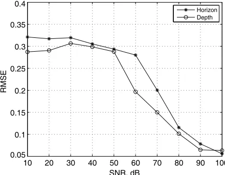
The above-mentioned is for noiseless circumstance. In reality, it is important that the reconstruction algorithm is robust under noise contamination. To do this, after the feature vectors are generated, they are successively corrupted by an additive Gaussian noise with mean value equal to zero and variance fixed according to the desired signal-to-noise ratio (SNR). We define the relative mean square error
-1.50 -1 -0.5 0 0.5 1 1.5
0.01 0.02 0.03 0.04 0.05 0.06 0.07 0.08 0.09 0.1
Horizon, m
Average Relative Error
Actual data Quadratic fitting curve
0 0.5 1 1.5 2 2.5 3 3.5 4
0 0.02 0.04 0.06 0.08 0.1 0.12 0.14
Depth, m
Average Relative Error
Actual data Quadratic fitting curve
(a) (b)
0 20 40 60 80 100 120 -1.5
-1 -0.5 0 0.5 1 1.5
Index
Horizon, m
Actual value Predicted value
0 20 40 60 80 100 120
-0.5 0 0.5 1 1.5 2 2.5 3 3.5 4 4.5
Index
Depth, m
Actual value Predicted value
(a) (b)
Figure 5. Actual versus predicted values of the (a) x-coordinate and (b) y-coordinate of the target center with 0.95 confidence intervals (⊥ denoted error bars).
10 20 30 40 50 60 70 80 90 100
0.05 0.1 0.15 0.2 0.25 0.3 0.35 0.4
SNR, dB
RMSE
Horizon Depth
Figure 6. RMSE as a function of SNR for horizontal and depth value of the target center.
(RMSE) for the position, i.e., x-coordinate and y-coordinate:
Rx =
1
Ntest Ntest
i=1
xi−x˜i lx
2
(19)
Ry =
1
Ntest Ntest
i=1
yi−y˜i ly
2
(20)
where Ntest is the number of the samples in testing dataset. (xi, yi), (˜xi,y˜i) are the ith actual and
5. CONCLUSION
In this paper, a machine-learning approach called RVM for through-wall detection has been proposed. It is characterized by its ability to capture the underlying physic of the system simply by examination of the inputs and outputs of the system. In such a framework, RVM has been shown to provide an effective method for through-wall scenario. The effectiveness of the approach has been preliminarily assessed by considering a two-dimension geometry in noiseless as well as noisy conditions. The obtained results of this technique can detect the target through a wall.
In this paper, we consider the feature vector extracted from the scattered field introduced by the target as input fed to the RVM predictor. However, in through-wall scenario, the collected field at each observation location is not only the scattered field from the target, but also the reflected field caused by walls. Hence, background removal is becoming an important issue. Consequently, the process of background removal will limit auto-focusing of the through-wall imagery under unknown wall characteristic.
ACKNOWLEDGMENT
We want to thank the helpful comments and suggestions from the anonymous reviewers. This work was supported by the National Natural Science Foundation of China (Grant No. 61071022), Graduate Student Research and Innovation Program of Jiangsu Province (Grant No. CXZZ11 0381) and Nanjing University of Posts and Telecommunications Foundation, China (Grant No. NY208037).
REFERENCES
1. Song, L. P., C. Yu, and Q. H. Liu, “Through-wall imaging (TWI) by radar: 2-D tomographic results and analyses,” IEEE Trans. Geosci. Remot. Sens., Vol. 43, No. 12, 2793–2798, 2005. 2. Baranoski, E. J., “Through-wall imaging: Historical perspective and future directions,” J. Frank.
Inst., Vol. 345, No. 6, 556–569, 2008.
3. Ferris, D. D. and N. C. Currie, “Survey of current technologies for through-the-wall surveillance (TWS),” Proc. SPIE, Vol. 3577, 62–72, 1999.
4. Soldovieri, F., F. Ahmad, and R. Solimene, “Validation of microwave tomographic inverse scattering approach via through-the-wall experiments in semicontrolled conditions,”IEEE Geosc. Rem. Sens. Lett., Vol. 8, No. 1, 123–127, 2011.
5. Ahmad, F., M. G. Amin, and S. A. Kassam, “Synthetic aperture beamformer for imaging through a dielectric wall,”IEEE Trans. Aerosp. Electron. Syst., Vol. 41, No. 1, 271–283, 2005.
6. Ahmad, F., M. G. Amin, and G. Mandapati, “Autofocusing of through-the-wall radar imagery under unknown wall characteristics,” IEEE Trans. on Image Proc., Vol. 16, No. 7, 1785–1795, 2007.
7. Dehmollaian, M. and K. Sarabandi, “Refocusing through building walls using synthetic aperture radar,”IEEE Trans. Geosci. Remot. Sens., Vol. 46, No. 6, 1589–1599, 2008.
8. Soldovieri, F. and R. Solimene, “Through-wall imaging via a linear inverse scattering algorithm,” IEEE Geosc. Rem. Sens. Lett., Vol. 4, No. 4, 513–517, 2007.
9. Soldovieri, F., R. Solimene, and G. Prisco, “A multiarray tomographic approach for through-wall imaging,”IEEE Trans. Geosci. Remot. Sens., Vol. 46, No. 4, 1192–1199, 2008.
10. Chew, W. C. and Y. M. Wang, “Reconstruction of 2-dimensional permittivity distribution using the distorted born Iterative method,”IEEE Trans. Med. Imag., Vol. 9, No. 2, 218–225, 1990. 11. Cui, T. J., W. C. Chew, A. A. Aydiner, and S. Y. Chen, “Inverse scattering of two-dimensional
dielectric objects buried in a lossy earth using the distorted born iterative method,” IEEE Trans. Geosci. Remot. Sens., Vol. 39, No. 2, 339–346, 2001.
13. Kim, Y. and H. Ling, “Through-wall human tracking with multiple doppler sensors using an artificial neural network,” IEEE Trans. Antennas Propagat., Vol. 57, No. 7, 2116–2122, 2009. 14. Kim, Y. and H. Ling, “Human activity classification based on micro-doppler signatures using a
support vector machine,”IEEE Trans. Geosci. Remot. Sens., Vol. 47, No. 5, 1328–1337, 2009. 15. Wang, F. F. and Y. R. Zhang, “A real-time through-wall detection based on support vector
machine,” Journal of Electromagnetic Waves and Applications, Vol. 25, No. 1, 75–84, 2011. 16. Tipping, M. E., “Sparse Bayesian learning and the relevance vector machine,”Journal of Machine