BIROn - Birkbeck Institutional Research Online
Ng, S.-L. and Paterson, Maura B. (2018) Functional repair codes: a view
from projective geometry. Working Paper. Birkbeck, University of London,
London, UK.
Downloaded from:
Usage Guidelines:
Please refer to usage guidelines at or alternatively
Functional repair codes:
a view from projective
geometry
By
S.-L. Ng and M.B. Paterson
Functional repair codes: a view from projective geometry
Siaw-Lynn Ng
∗, Maura Paterson
†October 29, 2018
Abstract
Storage codes are used to ensure reliable storage of data in distributed systems. Here we consider functional repair codes, where individual storage nodes that fail may be repaired efficiently and the ability to recover original data and to further repair failed nodes is pre-served. There are two predominant approaches to repair codes: a coding theoretic approach and a vector space approach. We explore the relationship between the two and frame the later in terms of projective geometry. We find that many of the constructions proposed in the literature can be seen to arise from natural and well-studied geometric objects, and that this perspective gives a framework that provides opportunities for generalisations and new constructions that can lead to greater flexibility in trade-offs between various desirable prop-erties. We also frame the cut-set bound obtained from network coding in terms of projective geometry.
We explore the notion ofstrictly functionalrepair codes, for which there exist nodes that
cannot be replaced exactly. Currently only one known example is given in the literature, due to Hollmann and Poh. We examine this phenomenon from a projective geometry point of view, and discuss how strict functionality can arise.
Finally, we consider the issue that the view of a repair code as a collection of sets of vector/projective subspaces is recursive in nature and makes it hard to visualise what a collection of nodes looks like and how one might approach a construction. Here we provide another view of using directed graphs that gives us non-recursive criteria for determining whether a family of collections of subspaces constitutes a function, exact, or strictly functional repair code, which may be of use in searching for new codes with desirable properties.
1
Introduction
The growth of data and an increasing reliance on digital information have led to much research into ensuring that data can be stored reliably. One predominant solution is the use of storage codes for distributed storage systems: a database is coded and stored in multiple nodes (servers)
∗Information Security Group, Royal Holloway, University of London, Egham, Surrey, TW20 0EX, U.K. [email protected].
in such a way that if a number of nodes fail, the data can still be recovered from the functioning nodes. One technique used in practice (for example, RAID [15], Total Recall [2]) is that of erasure coding: for instance, MDS codes such as the Reed-Solomon code ([12]) can be used to ensure that any number of node failures up to a certain threshold does not impede therecovery of the entire database. However, many distributed storage systems also require additional resilience properties. In particular, we may want to mitigate node failures: if a node should fail, we would like to
repair it using information in some of the functioning nodes so that the the recovery property of the system still holds. Clearly one could do that by simply recovering the entire database and re-encoding it. This involves a sometimes unacceptable overhead in storage and communication. Much work has been done to minimise the amount of data to be stored and the amount of data to be transmitted for repair. Using techniques from network coding, Dimakis et al. ([3]) showed that one could significantly reduce the amount of data to be communicated for repair and showed that there is a tradeoff between storage and repair efficiency. Since then much work has been done on modelling and constructing efficient repair codes. Here we consider two strands of this work.
In [16], Rashmiet al. proposed a product-matrix framework for repair codes. This is an essentially coding theoretic approach, where the database is treated as messages that are encoded using a generator matrix. The resulting codewords are then stored in individual nodes. Using this framework, repair codes can be constructed with parameters that sit on various points on the storage-repair tradeoff curve. On the other hand, in [8], Hollmann and Poh viewed a repair code as a collection of sets of subspaces of a vector space. Recovery corresponds to generating the vector space while repair corresponds to generating a subspace. In this paper (Section 2.3) we explore the relationship between these two models and motivate the interpretation of the vector space model in terms of projective geometry. We will see that many constructions arise naturally from looking at repair codes from a projective geometric point of view (Section 3) and these include the constructions in [8, 17]. We also frame a special case of the cut-set bound that Dimakis et al. obtained from network coding technique ([3]) in terms of projective spaces. This proves to be relatively straight forward compared to the original proof.
There are broadly speaking two types of repair. In exact repair, if a node fails then the new node constructs exactly the same symbols that the failed node stored. In functional repair, the new node does not necessarily contain the same symbols as the failed node, but the set of nodes after repair should remain a repair code: one should still be able to recover the original database, and future repair should be possible. We will call a functional repair code that does not admit exact repair a strictly functional repair code. In this paper we will also clarify what exact and functional repair means. One interesting question is whether there exists strictly functional repair codes. In Section 3 we see that there are repair codes that can be both functional and exact, but in [8] there is a construction that is strictly functional. This appears to be the only example in the literature so far. Another aim of this paper (Sections 3.2.2 and 4) is to examine this structure from a projective geometry point of view and to see if it can be generalised. We give another example of a strictly functional repair code which arises from a familiar structure in projective planes (Section 3.1.1).
This models the repair property, insisting that future repairs must be possible. However, this recursive nature makes it hard to visualise what a collection of admissible sets look like: it is hard to discern the “global view” of the whole set of nodes from the “local view” of individual node repairs. In the construction of this strictly functional repair code, a description is given that uses symmetry to bypass the recursiveness of the definition. This naturally leads to the question of whether this can be generalised, and also motivates another view using directed graphs. We discuss exact and functional repairs in terms of the properties of these graphs in Section 6.
We will make these aims more precise when we introduce notation. We would like to note that constructing new efficient storage codes is not the primary focus of this work, even though many objects in projective geometry appears to offer good repair as well as flexibility in terms of resilience and trade-offs between locality and repair. We intend rather to clarify the definition and properties of functional repair codes, and to consider their possible relationship with other combinatorial objects.
The structure of this paper is as follows: we will give definitions and introduce notation in Section 2, and consider some motivation for phrasing things in terms of projective geometry (Section 2.3). In Section 3 we examine functional repair codes arising from projective geometry objects, and study in further detail the strictly functional repair code of [8] in Sections 4 and 5. In Section 6 we consider functional repair codes as digraphs, and in Section 7 we discuss further work.
2
Definitions and basic properties
An (m;n, k, r, α, β)-functional repair code storesminformation symbols from some finite alphabet
F, encoded acrossnstorage nodes. Each storage node can holdαsymbols. The following properties hold:
(I) (Recovery)
The original information can be recovered from the data stored on k nodes (the recovery set).
(II) (Repair)
If a storage node fails then a newcomer node contacts some set of r surviving nodes (the repair set) and downloads β symbols from each of these r nodes. From these symbols the newcomer node constructs and storesα symbols in such a way that (I) holds and (II) holds if another node fails.
We note that there is a dichotomy in the definition of the repair set: in some work (for example, [3, 16]) it is stipulated that the repair set is any set of r surviving nodes, while in others (for example, [8, 21]) it is only required that there existssomernodes to form the repair set. Similarly for the recovery set. We will continue this discussion after Definition 2.2.
(m;n, k, r, α, β)-functional repair code. A functional repair code that does not admit exact repair is a strictly functional repair code. (We will make these definitions more precise in what follows.) The focus of this paper is functional repair.
In [8] and various subsequent work, a functional repair code is viewed as a collection of sets of subspaces of an m-dimensional vector space over a finite field Fq. The underlying storage codes
work as follows:
• For i with 0≤i≤n−1, the ith node is assigned a vector space represented by a specified basis {vi
0,vi,. . . ,viα−1}.
• To store a message x = (x0, x1, . . . , xm−1) ∈Fmq , each node i with 0≤i≤n−1 stores the
α scalar values{x·vi
0,x·vi,. . . ,x·viα−1}.
• If the vector (1,0, . . . ,0) is in the span of a set of vectors {u0, . . . ,ut−1}, then the values
{x·u0, . . . ,x·ut−1} can be used to recover x0. For, if (1,0, . . . ,0) =Pti−=01aiui for ai ∈Fq,
then x0 = Pti−=01aix·ui. If the vectors {u0, . . . ,ut−1} span Fmq then the entire message x
can similarly be recovered from these values.
The properties of the storage code are hence determined by the relationship between the subspaces that correspond to the nodes, in particular, the spans and the intersections of these subspaces. The projective space PG(m−1, q) provides a very natural setting for studying spans and intersections in Fm
q . It can make the relationship between spaces easier to visualise and, furthermore, many
natural geometric structures in PG(m−1, q) have well-understood span/intersection properties that can be useful in constructing storage codes. In what follows we will translate the vector-space definitions of [8, Definitions 3.1, 3.2] into the language of projective vector-spaces. We will see that this provides new insight into existing constructions of repair codes, such as [8, 17], as well as suggesting useful frameworks for new construction of such codes.
Definition 2.1 ((r, β)-repair). Let Σ = PG(m−1, q) be an (m−1)-dimensional projective space over the finite field Fq. We say that we can obtain a subspace U0 of Σ from a set U of subspaces
of Σ by (r, β)-repair if there is an r-subset {Ui1, . . . , Uir} in U such that there exists a (β− 1)-dimensional subspace Wij ⊆Uij for eachij such that U0 ⊆ hWi1, . . . , Wiri.
Definition 2.2 (Functional repair codes). Let Σ = PG(m−1, q) and let A be a collection of (n−1)-sets U of (α−1)-dimensional subspaces of Σ such that:
(A) (Recovery)
For each setU ∈ Athere is a k-subset {Ui1, . . . , Uik}of the subspaces inU whose span is all of Σ.
(B) (Repair)
Given any (n−1)-setU ={U1, . . . , Un−1}in A, there exists an (α−1)-dimensional subspace
Un ⊂ Σ that can be obtained from U by (r, β)-repair, such that for every i = 1, . . . n−1,
We will call (Σ = PG(m−1, q),A) an (m;n, k, r, α, β)-functional repair code (or (m;n, k, r, α, β )-FRC for convenience).
HereAcorresponds to all possible sets ofn−1 subspaces that belong to the nodes remaining after a single node has failed. The repair property ensures that there is always a suitable subspace that can be constructed by (r, β)-repair from these nodes in order to construct a replacement for the node that has failed. Clearly here we require that there exists some recovery set andsome repair set, although in many of the constructions we describe in Section 3, repair and recovery can be effected by arbitrary sets. We will clarify each case as we go along.
To avoid triviality we assume that m, n ≥ 2, 1 ≤ k < n, k ≤ r ≤ n−1, 1 ≤ α ≤ m−1, and 1≤β≤α.
Definition 2.3. Let (Σ = PG(m−1, q),A) be an (m;n, k, r, α, β)-functional repair code. Ann-set
{U1, . . . , Un}of (α−1)-dimensional subspaces of Σ with the property that{U1, . . . , Un}\{Uj} ∈ A
for all j ∈ {1, . . . , n} is said to berepairable.
It is the repairable sets corresponding to (Σ,A) that can be used as storage codes; if any node fails, the repair property then ensures that the resulting (n−1)-set permits a new repairable set to be obtained through (r, β)-repair. Now we define exact and strictly functional repairs:
Definition 2.4 (Exact repair). Let (Σ = PG(m−1, q),A) be an (m;n, k, r, α, β)-functional repair code. We say that (Σ,A) is an exact repair code if for any repairable set {U1, . . . , Un} we have
the additional property that Ui can be obtained by (r, β)-repair from {U1, . . . , Un} \ {Ui} for any
Ui ∈ {U1, . . . , Un}.
We observe that if (Σ,A) is an exact repair code, then any for any repairable setR={U1, U2, . . . , Un},
the collection A0 = {R\ {U
i}|1≤ i ≤ n} has the property that (Σ,A0) is itself an exact repair
code.
Definition 2.5 (Strictly functional repair). Let (Σ = PG(m−1, q),A) be an (m;n, k, r, α, β )-functional repair code. We say that (Σ,A) is a strictly functional repair code if there exists a repairable set {U1, . . . , Un} for which there is a Ui ∈ {U1, . . . , Un} that cannot be obtained from
{U1, . . . , Un} \ {Ui}by (r, β)-repair.
2.1
Geometric interpretation of the cut-set bound
In [3], the cut-set bound of network coding is used to establish an upper bound on the the number of information symbols m that can be stored in an (m;n, k, r, α, β)-functional repair code. Here we interpret this bound in terms of finite projective geometry for the case n=r+ 1, β= 1.
Theorem 2.6. Let (Σ = PG(m−1, q),A) be a (m;r+ 1, k, r, α,1)-functional repair code. Then
m≤
k
X
i=1
min(α,(r−k) +i).
2
Proof. Each node i corresponds to a subspace Ui of Σ of dimension α−1, and any k of them
span PG(m −1, q). In particular, the spaces corresponding to the first k nodes span Σ, i.e.
hU1, U2, . . . , Uki= Σ. This implies that m−1 is at most kα−1.
Consider a repair of node 1. The repair property implies it is possible to choose one point P1
j
from each node j with 2 ≤ j ≤ r + 1 such that there is an (α−1)-dimensional subspace U0 1 contained in their span with {U0
1, U2, . . . , Ur+1}repairable. Since we require hU10, U2, . . . , Uki= Σ,
it follows that hU2, U3, . . . , Uk, Pk1+1, Pk1+2, . . . , Pr1+1i = Σ. This implies that m−1 is at most (k−1)α−1 + (r+ 1−k).
We now consider a repair of node 2. There exists a point P2
j in each node with j 6= 2 (including
P2
1 in U10) such that there is a (α−1)-dimensional subspace U20 contained in their span with
{U10, U20, . . . , Ur+1}repairable, and hU3, . . . , Uk, Pk1+1, Pk1+2, . . . , Pr1+1, P12, Pk2+1, Pk2+2, . . . , Pr2+1i= Σ. This implies that m−1 is at most (k−2)α−1 + (r+ 1−k) + (r+ 2−k).
We can repeat this process, continuing to replace eachUi in the set by a collection of repair points
whose inclusion ensures that the replacmentU0
i will be contained in the relevant span. After repair
of node i we have the result that m−1 is at most (k−i)α−1 +Pij=1(r+j−k). The bound on m−1 is lowered at each step until either we reach a point at which the number of additional points we have to add (r+i−k) is greater than α, or we have replaced replaced all ofU1, . . . , Uk
with the relevant repair sets of points. At this point we stop, and we have
m−1≤
k
X
j=1
min(α, r+j−k) !
−1,
so
m≤
k
X
j=1
min(α, r+j−k),
=
k−1 X
i=0
Generalising to β >1 is entirely straightforward: in each step of the proof we take β points per node rather than 1 point. This approach would also work in the n > r+ 1 case if we make the assumption thatanyset ofrnodes can be used for repair. This is the assumption made in [3, 16].
2.2
Performance measures for FRCs
In the definitions of Section 2 there is no stipulation on the size of A, nor on the number of (α−1)-dimensional subspaces in an (m;n, k, r, α, β)-functional repair code. Let N be the number of distinct (α−1)-dimensional subspaces used in A. We will consider bounds on the value of N in Section 6.
The commonly-studied measures of efficiency of an FRC are thestorage rateRs= nαm (the number
of message symbols divided by the total number of stored symbols)and the repair rate Rr = rβα
(the number of symbols required for the repaired node divided by the number of symbols requested in order to facilitate repair). The value rβ is called the repair bandwidth. Another performance metric is locality - the number of nodes to be contacted for repair, given byr.
Other performance metrics that we will not describe formally include availability, which is the number of disjoint repair sets for a node. Recent interest in this includes [19] where fractional repetition codes are used to construct codes with high availability and nodes are partitioned into clusters, each cluster providing a set of helper nodes to repair a failed node, and [25], where codes with different repair bandwidth for repair within clusters and across clusters are proposed.
The ability to repair multiple failures is also obviously of interest, and this may also be studied under different models, for example, [29, 30] study centralised repair (where repair is carried out in one location) and cooperative repair (where failed nodes may communicate) for multiple failures.
Much existing literature seeks to construct codes that optimise one or more of these measures ([3, 16, 23]). This is not the primary motivation of this paper, although we will examine the trade-offs that arise from the various possible construction choices we discuss. We will see that most geometrical constructions seem to have good repair rates but less than ideal storage rates; some of them offer a trade-off between repair rate and locality.
2.3
The product-matrix model
The other widely used model of (m;n, k, r, α, β)-functional repair codes is the product-matrix model [16] mentioned in the Introduction. In this model, theminformation symbols are formatted into anr×αmessage matrix, and the encoding process involves multiplication by ann×rencoding matrix. The resulting n×α matrix gives the symbols stored on each of the n nodes: row i of the matrix denotes the αsymbols stored in node i. This can be viewed as an instantiation of the vector space model of [8]: if the entries in the ith row of the encoding matrix are E
i1, Ei2, . . . Eir,
then the ith node corresponds to the subspace spanned by the vectors v
0,v1, . . . ,vα−1, where vj has the valuesEi1, Ei2, . . . , Eir in positionsjr+ 1 throughjr+rand 0 in the remaining positions.
2.4
Subpacketisation/vectorisation
We now consider a well-known example of an FRC that can be generated using the the product-matrix model with α= 1, together with the application of a technique proposed by Shanmugam
et al. for improving the repair bandwidth [24]. We will see that this example can be described very naturally in the projective geometry setting.
Example 2.7. [Scalar MDS code] A filex0. . . xm−1consisting ofmsymbols belonging to the field
Fps, pa prime power and s > 1, is stored acrossn storage nodes using an [n, m]-MDS code over
Fps. (This is referred to as ascalar MDS code.) Each storage node would then store exactlyα= 1 symbol of Fps. Now, if one storage node should fail, a repair would involve contacting r = m nodes, each contributing β = 1 symbol. Altogether it would take rβ = m symbols to repair one symbol.
Following the approach of Definition 2.2, the scalar MDS code construction translates to a collec-tion of npoints P0, . . . , Pn−1 in Σ = PG(m−1, ps), every mof which span Σ; this is precisely an
n-arc in PG(m−1, ps). Any failed node can only be obtained by a (m,1)-repair, since any given
point of the arc is not contained in the space spanned bym−1 further points of the arc. This is an (m;n, m, m,1,1)-functional repair code with storage rate Rs = mn and repair rate Rr= m1.
2
In [24] Shanmugam et al. proposed a “vectorisation” of MDS codes over fields of prime power in order to obtain a better repair bandwidth. “Vectorisation” or “subpacketisation” involves treating each symbol xi ∈Fps as s symbols of Fp. As a consequence, instead of having to downloading all the symbols in each node, one may be able to effect repair by downloading fewer symbols (from perhaps more nodes), resulting in a reduction of repair bandwidth.
To explore the vectorisation process more explicitly, letf(x) =a0+a1x+· · ·+as−1xs−1+xs be a primitive polynomial of degreesoverFpand letζ be a root off(x). Then every elementbofFps can be written asb=b0+b1ζ+· · ·+bs−1ζs−1,bi ∈Fp. Using this correspondence,b∈Fpscan be viewed as (b0, b1, . . . , bs−1) ∈ Fsp. This is the basis of the technique of field reduction used to construct
Desarguesian spreads of PG(sm−1, p) from the points of PG(m−1, ps) ([6, Section 4]). A point
(x0, x1, . . . , xm−1) in PG(m−1, ps), withxi ∈Fps viewed as (xi0, xi1, . . . , xis−1)∈Fsp, can be written as the point (x0
0, x01, . . . , x0s−1, x01, x11, . . . , x1s−1, . . . , x0m−1, xm1−1, . . . , xms−−11) in PG(sm−1, p). Now, take a point (p0, p1, . . . , pm−1)∈PG(m−1, ps) and all its multiples{(p0ζi, p1ζi, . . . , pm−1ζi | i= 0, . . . , ps −2}. Then the corresponding points of this set in PG(sm −1, p) form an (s−
1)-dimensional subspace. The set of all such (s−1)-dimensional subspaces partitions PG(m−1, ps)
and is a Desarguesian spread.
(The “vectorisation” process in [24] uses another map: each b ∈ Fps can be treated as a linear transformationx7→bx in Fps, sob can be described as an s×s matrix acting on the basis of Fps over Fp. Each element of the MDS code is thus replaced by its corresponding s×s matrix. This
process is equivalent to the field reduction construction of Desarguesian spreads described above.)
The “vectorised” functional repair code is now an (sm;n, m, r ≤ m, s, β)-functional repair code for some r and β and storage rate Rs = mn, repair rate Rr = rβs. It corresponds to a set of n
We give a small example to illustrate this principle:
Example 2.8. Takes = 3, k = 3, n = 5, we have a 5-arc in PG(2,8) (taking primitive element
ζ3 =ζ + 1):
1 0 0 0 1 0 0 0 1 1 1 1 1 ζ ζ2
.
This is an (m= 3;n= 5, k = 3, r = 3, α= 1, β = 1)-functional repair code withRs = 35, Rr= 13.
“Vectorisation” gives 5 planes in PG(8,2): each group of three rows are 3 points that span a plane. We call the planes U1, . . . , U5.
1 0 0 0 0 0 0 0 0
0 1 0 0 0 0 0 0 0
0 0 1 0 0 0 0 0 0
0 0 0 1 0 0 0 0 0
0 0 0 0 1 0 0 0 0
0 0 0 0 0 1 0 0 0
0 0 0 0 0 0 1 0 0
0 0 0 0 0 0 0 1 0
0 0 0 0 0 0 0 0 1
1 0 0 1 0 0 1 0 0
0 1 0 0 1 0 0 1 0
0 0 1 0 0 1 0 0 1
1 0 0 0 0 1 0 1 0
0 1 0 1 0 1 0 1 1
0 0 1 0 1 0 1 0 1
.
This is now an (m = 9;n = 5, k = 3, r = 5, α= 3, β = 2)-functional repair code. If U1 fails, one could repair U1 by downloading the following points:
• R21 = (000 110 000),R22 = (000 011 000) from U2,
• R31 = (000 000 110),R32 = (000 000 011) from U3,
• R41 = (110 110 110),R42 = (011 011 011) from U4,
Then we can get (010 000 000) = R51+R21 +R22+R32, (110 000 000) = R41+R21+R31, and (011 000 000) =R42+R22+R32. This gives us U1.
In the scalar version, to repair one point (9 bits of information) we need to use three points (27 bits). The repair rate is therefore 1/3. In the “vectorised” version, to repair one subspace (27 bits) we need to use 8 points (72 bits). The repair rate is thus 3/8 > 1/3. (Or 3/7 if we don’t
mind lopsidedness.) 2
The motivation in [24] is to obtain a better repair rate, which the example illustrated. In addition, we see that this process has a natural counterpart in projective geometry that is also intuitive.
Much work has been done further along these lines with some variations. For instance, [1] studies the lower bound forα(the “sub-packetisation”) in MSR codes that allow “repair-by-transfer”, that is, symbols from the remaining functioning nodes are downloaded directly without computation during repair, and [26] provides further examples of codes reaching the lower bound for α for different values of localityd(rin this paper). Meanwhile, [4] studies trading off repair bandwidth for better sub-packetisation, and [18] also provides constructions for MSR codes achieving the lower bound for αfor “repair-by-transfer”.
3
Projective geometric constructions of functional repair
codes
We will examine some existing constructions and also some constructions that arise naturally from looking at functional repair codes from a projective geometric point of view. The construction of a vector space/projective geometric functional repair code involves choosing both the dimensions of the spaces corresponding to the nodes, and selecting which subspaces of these dimensions to use. The properties of the code are determined entirely by the manner in which the various spaces intersect. The advantage of the geometric perspective is that many classical geometric objects have nice, well-understood properties in terms of how spaces embedded in these objects intersect. We will see that many existing constructions in the literature can be viewed as arising from classical geometric objects in this way.
3.1
Constructions using intersecting subspaces.
We begin by considering the simplest possible case for intersecting subspaces, that of lines in a plane, then use the results obtained to suggest useful constructions in higher dimensions.
3.1.1 Dual arcs
A neat construction of an exact repair code can be obtained from three lines in a plane:
Example 3.1. [Three lines in a plane.] Any three non-concurrent lines in a plane will give an exact repair code: letl1,l2,l3be three non-concurrent lines in PG(2, q), and letAbe the collection of the sets of pairs of distinct lines {li, lj} ⊆ {l1, l2, l3}. Then A is an (m = 3;n = 3, k = 2, r = 2, α= 2, β = 1)-functional repair code.
We may coordinatise l1, l2,l3 as:
l1 : h(1,0,0),(0,1,0)i,
l2 : h(0,1,0),(0,0,1)i,
l3 : h(1,0,0),(0,0,1)i. A (2,1)-repair forl3, for example, ish(1,0,0)∈l1,(0,0,1)∈l2i.
Here the storage rate Rs= 1/2 and the repair rate isRr = 1. 2
This example tolerates a single node failure. In order to protect against additional failures we may desire schemes permitting more nodes. We can achieve this by generalising the idea of Example 3.1 to a larger set of lines: adual arc in a a projective plane of order qis a set of N ≤q+ 1 lines, no three concurrent.
Theorem 3.2. LetL be a collection ofN ≥ 3 lines of a projective plane Σ such that no three of them are concurrent. Let Abe the collection of (N −1)-tuples of distinct lines of L. Then (Σ,A) is an (m = 3;n = N, k = 2, r = 2, α = 2, β = 1)-functional repair code that can tolerate up to
N −2 node failures if N >3. 2
Proof. Any subset of three nodes in L can be considered to be an exact repair code, as seen in Example 3.1. Thus, provided two nodes survive, any failed node can be recovered by exact repair.
Construction 3.3 (Dual arcs in a plane). Let C be a nonsingular conic in PG(2, q) with q an odd prime power. Let L be a subset of the tangents to C with |L| = n, 3 ≤ n ≤ q+ 1. Then
L is a dual arc in PG(2, q) ([6]). Let A be the collection of pairs of distinct lines of L. Then by Theorem 3.2, we have that (Σ,A) is an (3;n,2,2,2,1)-functional repair code that can tolerate up to n−2 node failures (ifn >3), with storage rate Rs= 3/2n≤1/2 and repair rate 1.
Example 3.4. [Planes in PG(3, q).] Consider a dual arc in PG(3, q): a set of q+ 1 planes, any 4 meeting trivially. (So 2 planes meet in a line, 3 planes meet in a point.)
Take 3 of the planes π1, π2, π3. If π3 fails, repair to π30 using lines li ∈πi, i= 1,2. This gives a
(m= 4; 3≤n≤q+ 1, k= 2, r= 2, α= 3, β = 2)-functional repair code. For example,
π1 : x0 = 0,
π2 : x1 = 0,
π3 : x2 = 0.
If π3 fails, for example, it can be repaired by (2,2)-repair using lines l1 = {(0, x1,0, x3)|x1, x3 ∈
Fq, not both zero.} ∈ π1 and l2 = {(x0,0,0, x3) | x0, x3 ∈ Fq, not both zero.} ∈ π2. This gives an (m = 4;n = 3, k = 2, r = 2, α = 3, β = 2)-functional repair code, with Rs = 4/3n = 4/9,
Rr = 3/4.
On the other hand, we could take 4 planes
π0 : x0 = 0,
π1 : x1 = 0,
π2 : x2 = 0,
π3 : x3 = 0.
If π3 fails, it can be repaired by (4,1)-repair, usingP0 = (0,1,0,0)∈π0,P1= (0,0,1,0)∈π1, and
P2 = (1,0,0,0) ∈π2. This gives an (m = 4;n = 4, k = 2, r = 3, α= 3, β = 1)-functional repair code, with Rs = 4/3n= 1/3 and better repair rate,Rr = 1. 2
There are two important features in the simple construction of Example 3.4: the ability to trade off locality and repair bandwidth without having to make a decision during the set up, and the ability to repair multiple failures. Before we discuss this in more detail, we give the general construction:
Construction 3.5. Take a dual arc in PG(m− 1, q): a set of q + 1 hyperplanes, any m of
which meet trivially. We may take the set of hyperplanes in a dual normal rational curve {Ht =
[1, t, t2, . . . , tm−1] : t ∈ F
q} ∪ {H∞ = [0,0, . . . ,0,1]}, where [z0, z1, . . . , zm−1] denotes the set of points {(x0, x1, . . . , xm−1)|z0x0+z1x1+· · ·+zm−1xm−1= 0}.
However, to make the description of the trade-off clearer, we will take an m-subset of these hyperplanes and coordinatise them as follows, writing ei to denote the point with a 1 in position
i and 0 everywhere else:
Hi :xi = 0, that is, Hi =hej, |j ∈ {0, . . . , m−1} \ {i}i.
This gives an (m;n = m, k = 2, r = dmβ−1e, α = m−1, β)-functional repair code with Rs = nαm
and Rr = mm−−1+1δ, whereδ = 0 if β|m−1. Otherwise δ= β−∆ where ∆ = m−1 modβ. Here
For simplicity we describe what happens if H0 fails. An (r, β)-repair can be performed, with
r=dmβ−1e, with each of the active Hi contributingβ points as follows:
H1 → e2, . . . , eβ+1,
H2 → eβ+2, . . . , e2β+1, ...
Hi → e(i−1)β+2, . . . , eiβ+1, ...
Hdm−1
β e → e(dmβ−1e−1)β+2, . . . , em−1, e1.
Clearly at any repair one could choose the localityr to suit the circumstances. In [17] a construc-tion was given that also allows such a trade-off - one can choose between minimum bandwidth repair or low locality repair, by assigning the subspaces accordingly, but this assignment has to be determined at set up. Construction 3.5 allows the trade-off to be performed at each repair according to the network conditions.
Construction 3.5 also tolerates multiple node failures: we can choose m ≤ n ≤ q+ 1, and any failure of up to n−2 nodes still allows recovery and repair. It also gives high availability. For example, when we consider the special case of Construction 3.3 using dual arcs in planes, we see that any line can be repaired using any pair of lines, so that many sets of nodes can be used to repair a failed node.
We note also that if we start with n < q + 1, additional nodes can be created by accessing information from some existing nodes using the repair process. This may be useful if resilience requirements change during the lifetime of the storage system.
3.1.2 Concurrent lines and strictly functional repair
The use of dual arcs in constructing functional repair codes is appealing due to the high availability that results. However Example 3.1 also prompts another question: what happens if we allow sets of nodes that correspond to concurrent lines? In Constructions 3.3 and 3.5, the spaces assigned to nodes correspond to hyperplanes in the underlying space. This means their pairwise intersections are well understood: any two hyperplanes of PG(m−1, q) intersect in a space of dimensionm−3. The use of the dual arcs enables us to control the way in which the spaces corresponding to larger sets of nodes intersect: any t of them intersect in a space of dimension m−1−t. However, we may wish to consider constructions where more general patterns of intersection are allowed (for example, in order to permit more thanq+ 1 nodes).
In order to explore what happens when more general patterns of intersection occur, we return to the case of lines in the plane, and consider collections of lines that include sets of three concurrent lines. The following example shows this takes us into the realm of strictly functional repair codes:
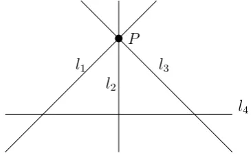
Example 3.6. [A strictly functional repair code.] Let l1, l2, l3, l4 be four lines of Σ = PG(2, q),
Figure 1: A strictly functional repair code in PG(2, q). P l1 l2 l3 l4
1.) Let A be the collection of pairs of lines {li, lj}, i, j ∈ {1,2,3,4}, i 6= j. Then (Σ,A) is am
(m= 3;n= 3, k= 2, r = 2, α= 2, β = 1)-functional repair code which is strictly functional repair code.
This is because there is a set{l1, l2, l3}with {l1, l2},{l1, l3},{l2, l3} ∈ Abutl3 cannot be obtained
from {l1, l2}by (2,1)-repair. 2
As far as we are aware, this appears to be the only other example of a strictly functional repair code in the literature, apart from an example due to [8] that we will discuss in Section 3.2.2.
3.1.3 Grassmann varieties
The constructions we discussed in Section 3.1.1 all involve subspaces that are hyperplanes of the ambient space. This represents one extreme point of the possible trade-off between low repair bandwidth and flexibility of repair at the cost of high storage. Using smaller dimensional spaces both reduces the storage overhead, and allows for greater flexibility in terms of the size of pairwise intersections between the spaces. In this environment where greater flexibility is possible, this implies that the spaces must be chosen carefully to achieve the desired intersection properties. Here we consider an example of a construction from [17]. It uses subspace codes constructed from Grassmann varieties in vector spaces. We will describe it from the point of view of projective geometry, in order to see how known properties of Grassman varieties make it possible to choose collections of subsets with suitable intersections.
Let b ≥ 2 and t ≤ b be integers. Consider Πt, a t-dimensional projective subspace of PG(b, q).
Let the points X0, . . . , Xt be a basis for Πt. Write Xi = (xi0, xi1, . . . , xib) and let MΠt be the (t+ 1)×(b+ 1) matrix
MΠt = X0 X1 ... Xt = x0
0 x01 . . . x0b
x1
0 x11 . . . x1b
... ... ...
xt
0 xt1 . . . xtb
.
i0, . . . , it. Let V be the set of bt+1+1
subsets {i0, . . . , it} of {0,1, . . . , b}, ordered in some way.
Let φ(MΠt(i0, . . . , it)) be defined as det(MΠt(i0, . . . , it)). Then φ(MΠt) is defined as a point in PG(B, q), whereB = tb+1+1−1, and thejth position ofφ(MΠt) isφ(MΠt(i0, . . . , it)) with{i0, . . . , it}
in the given order in V.
For example, take t= 1,b= 3. Suppose Π1 is a line in PG(3, q) with basis points (x0, x1, x2, x3), (y0, y1, y2, y3), and
MΠ1 =
x0 x1 x2 x3
y0 y1 y2 y3
.
Then φ(MΠ1) is a point in PG(5, q) given by
(x0y1−x1y0, x0y2−x2y0, x0y3−x3y0, x1y2−x2y1, x1y3−x3y1, x2y3−x3y2).
We call these Grassmann coordinates (or Pl¨ucker coordinates, when t = 1). The set of points in PG(B, q) corresponding to all thet-dimensional subspaces of PG(b, q) is called the Grassmannian, or the Grassmann variety of the t-spaces of PG(b, q). We will concentrate on the case t= 1 here and refer the reader to [7, Chapter 24] for more details and for the general case.
For t= 1, the lines of PG(b, q) are mapped to points of PG(B, q), B= b+12 −1. The q2+q+ 1 lines lying on a plane in PG(b, q) are mapped to a plane in PG(B, q) - the collection of such planes in PG(B, q) are called the Greek spaces. Theqb−1+qb−2+· · ·+b+ 1 lines through a point in PG(b, q) are mapped to a (b−1)-dimensional subspace in PG(B, q) - the collection of such subspaces are called the Latin spaces. Two Latin (Greek) spaces meet in at most one point, and a Latin and a Greek space meet in either a line or the empty set. If there are three distinct Latin (Greek) spaces π, π0, π00 such that their pairwise intersections are distinct points, then any other Latin (Greek) space ¯π having distinct points in common with π and π0 will also has a point in common withπ00. These properties allow the construction of the functional repair codes described in [17].
Construction 3.7 (Grassman variety construction [17]). The storage nodes V0, . . . , Vn−1 are associated with pointsP0, . . . , Pn−1 in PG(b, q). Each pointPi can be associated with a collection
of lines through that point, which, in turn, gives a (b−1)-dimensional subspaceMi in PG(B, q).
The recovery and repair properties then depend on how the points Pi are chosen: every b of the
Mi should span PG(B, q), and if an Mi should fail, one should be able to obtain it by some (r, β
)-repair. In [17], it is shown that this can be a (b,1)-repair or a (c, b)-repair for anyc|b. This gives an (m = B+ 1;n, k = b, r = b, α = b, β = 1)-functional repair code (or an (m = B+ 1;n, k =
b, r=c, α=b, β =b)-functional repair code for any c|b), where B= bt+1+1−1, t≤b.
Consider again the example witht= 1, b= 3. One could take n≥4 points in PG(3, q) such that no 4 points lie in a plane (an n-arc). The corresponding Grassmannian would then consist of n
planes in PG(5, q) with the property that every pair of planes meet in a point, and for any plane, the points of intersection with the other n−1 planes form an (n−1)-arc on the plane. It is then clear that any three planes would span PG(5, q), while any plane can be obtained by (3,1)-repair. This gives a repair rate of 1, and a storage rate of 2
n ≤
3.1.4 Segre varieties
Another class of varieties having subspaces with specific intersection properties are the Segre varieties. These can also be used to construct functional repair codes with intersecting subspaces. It gives storage rateRs = 12, and has some restrictive recovery properties, but may still be of some
interest.
A Segre variety SVs,t in PG((s+ 1)(t+ 1)−1, q) is defined as follows:
Let St be a t-dimensional projective space PG(t, q) and Ss be an s-dimensional projective space
PG(s, q). Then
SVs,t = {(y0z0, y0z1, . . . , y0zs;y1z0, y1z1, . . . , y1zs;. . .;ytz0, ytz1, . . . , ytzs)|
(y0, y1, . . . , yt)∈St, (z0, z1, . . . , zs)∈Ss}.
SVs,t consists of two opposite systems of subspaces Σ1, Σ2: Σ1 consists of qs+qs−1+· · ·+q+ 1 mutually skew t-dimensional subspaces, and Σ2 consists of qt +qt−1+· · ·+q+ 1 mutually skew
s-dimensional subspaces. Each subspace in Σ1 meets a subspace in Σ2 in exactly one point.
Example 3.8. Suppose s=t= 1. ThenSV1,1 is a hyperbolic quadric in PG(3, q) which consists of (q+ 1)2 points lying on 2(q+ 1) lines. These lines form the two opposite systems of subspaces, each consisting of q+ 1 mutually skew lines. If we take two lines from each system, then if one line fails it can always be repaired by (2,1)-repair from the two lines from the opposite system. For recovery, however, we must have k= 2 lines from the same system. The collection of 3-subsets of these 4 lines gives an (m= 4;n = 4, k= 2, r = 2, α= 2, β = 1)- functional repair code (with the possibility of adding more nodes by the repair process), with Rs= 12 andRr = 1.
This example illustrates the importance of the assumption of arbitrary recovery and repair sets in the cut-set bound: Theorem 2.6 says that m ≤3 for (k, rα, β) = (2,2,2,1). Here we achieve
m= 4, but the pairs of lines that constitute a recovery set are more restrictive. 2
This can be generalised to SVt,t, t ≥ 1: take t+ 1 t-dimensional subspace from Σ1, and t+ 1
t-dimensional subspaces from Σ2. Any one subspace may be obtained by (t+ 1,1)-repair from the t + 1 subspaces in the opposite system. For recovery, as before, we must have k = t+ 1 subspaces from the same system. The collection of (2t+ 1)-subsets of these 2t+ 2 subspaces gives an (m= (t+ 1)2;n= 2(t+ 1), k=t+ 1, r =t+ 1, α=t+ 1, β = 1)- functional repair code (again, with the possibility of adding more nodes by the repair process), withRs = 12 and Rr= 1.
3.2
Constructions using non-intersecting subspaces.
3.2.1 Spreads and partial spreads
Another natural object to look at when one considers projective space constructions is spreads and partial spreads.
Theorem 3.9. Let S be a regular spread in PG(3, q). Letl1, l2,l3 be three lines of S and let R be the (unique) regulus containing them. Let l4 ∈ S \ R. Then li4 can be obtained from li1, li2,
li3 by (3,1)-repair, {i1, i2, i3, i4}={1,2,3,4}. 2
Proof. It is clear that any three of l1, . . . , l4 are contained in a regulus that does not contained the fourth line, so without loss of generality it suffices to prove that l4 can be obtained from l1,
l2, l3 by (3,1)-repair.
Let Q1 be any point on l4. Letl5 be the transversal through Q1 to l2, l3 - this line exists and is unique. Let P2 =l5∩l2 andP3 =l5∩l3.
Now consider {l1, l3, l4}. There is a unique regulus containing them but not l2. Let l6 be the transversal to them through P3. Let P1 =l6∩l1 andQ2 =l6∩l4. (We know thatQ1 6=Q2 since otherwise l5 =l6 andl6 meets all four lines, which means all four lines are in a regulus.)
Now consider the space spanned byP1,P2,Q1,Q2,π=hP1, P2, Q1, Q2i. SinceP2Q1∩P1Q2= P3,
π is a plane. So P1P2 andl4 are both lines in π and thereforeP1P2 meetsl4 in a point Q3. Hence
l4 ⊆ hP1 ∈l1, P2 ∈l2, P3 ∈l3i and thus is obtained froml1, l2,l3 by (3,1)-repair.
Construction 3.10. [8, Example 2.1] The collection of pairs of distinct lines from {l1, l2, l3, l4} forms an (m= 4;n = 4, k= 2, r = 3, α= 2, β = 1)-functional repair code which has Rs = 12 and
Rr = 23.
For example, we may choose l1,l2, l3 to be
l1 = h(1,0,0,0),(0,0,1,1)i,
l2 = h(0,1,0,0),(1,0,0,1)i,
l3 = h(0,0,1,0),(1,1,0,0)i. These are lines on the quadric/regulus
x0x2−x0x3−x1x2−x2x3+x23= 0. (The other lines of the regulus are h(1,0, y,1),(1, y,0,0)i.)
We can take l4 to be h(0,0,0,1),(0,1,1,0)i, which does not belong to this regulus.
A natural generalisation of such a construction would be to take planes in spreads in PG(5, q). Indeed, in Section 2.3 a construction is given using elements of an (s−1)-spread in PG(sm−1, q). In [9, 10, 13, 14], regulart-spreads in PG(m−1, q) are used to give (m;k≤n ≤ 2m−1
2t+1−1, k= mα, r =
2, α = t+ 1, β = α)-functional repair codes. These functional repair codes have the additional property of allowing repairs of multiple node failures simultaneously. For example, in [14], up to n−1
2 failed nodes can be repaired simultaneously. This follows from the property of regular spreads, where one can always choose two spread elements that span a subspace that contains a third given element.
in Section 3.1.4 where elements are taken from both systems of subspaces of a Segre variety, here we only take subspaces from one system of subspaces, and these are mutually skew. Consider again an SVs,t as described in Section 3.1.4. For every point in St, there is a corresponding s
-dimensional subspace belonging to Σ2 in SVs,t. Take a t0-dimensional subspace V0 of PG(t, q),
t0 ≤t, and consider Σ0, thes-dimensional subspaces contained inSV
s,tcorresponding to the points
ofV0. Then, any subspace W in Σ0 can be obtained by (2, s+ 1)-repair from two other subspaces in Σ0: suppose W corresponds to the point P ∈ V0, pick a point P0 ∈ V0 and another point
P00∈V0 collinear withP andP0. Then the subspaces in Σ0 corresponding toP0 andP00 will span a subspace containing W. Let n = qt0q+1−1−1. The collection of (n−1)-subsets of s-dimensional subspaces from Σ0 gives an (m= (s+ 1)(t+ 1);n, k = t+ 1, r = 2, α= s+ 1, β = α)-functional repair code.
3.2.2 Focal spreads
Let Σ2t−1 = PG(2t−1, q), t > 1, and let St be a (t−1)-spread in Σ2t−1. Let L be an element of St. Let Σt+d−1, t > d, be a (t+d−1)-dimensional subspace of Σ2t−1 that contains L. Then
{L} ∪ {M0 = M ∩Σ
t+d−1 | M ∈ St \ {L}} is a focal spread consisting of the focus L, and the
(d−1)-dimensional subspaces M0 partitioning the points of Σ
t+d−1 not in L. Focal spreads are described in greater details in [11].
In [8] an (m= 5;n = 4, k = 3, r = 3, α= 2, β = 1)-functional repair code was constructed using focal spreads with t = 3,d= 2: a 2-spread in PG(5,2), intersected by a 4-space, the focus being a plane, and there are 8 lines partitioning the points not in the plane. The storage code consists the collection of 3-subsets of these 8 lines.
This can clearly be generalised. For example, using t = 4, d = 2, we have the storage code being 16 lines partitioning the set of points of a 5-dimensional space that are not contained in the focus, which is a 3-dimensional space. A computer search shows that a line cannot be obtained by (3,1)-repair but can be obtained by (4,1)-repair, making this an (m = 6;n = 16;k = 3, r = 4, α= 2, β = 1)-functional repair code.
However, the example in [8] turns out to be strictly functional, while our generalisation allows both functional and exact repair. Indeed, this appears to be the only strictly functional repair code that is known (apart from Example 3.6). In the next section we prove this property and examine the structure further.
4
Anatomy of a strictly functional repair code
In [8, Example 2.2 and Section VI], an (m= 5;n= 4, k= 3, r = 3, α= 2, β = 1)-functional repair code was given which turns out to be a strictly functional repair code. This is constructed using focal spreads and is described in Section 3.2.2. Here we prove that it is strictly functional, and consider whether it can be generalised.
Definition 4.1. Let Σ = PG(4, q) and letA be a set of 3-tuplesU of lines such that (a) (Recovery) For everyU ∈ A, the 3 lines in U span PG(4, q).
(b) (Repair) For each U = {U1, U2, U3} there is a point Pi on Ui, i= 1,2,3, such that there is
another line U4 ⊆ hP1, P2, P3i, and Ui0 =U ∪ {U4} \ {Ui}, i= 1,2,3, again belongs to A.
We will give a brief description of this construction in terms of projective spaces. We will describe the lines using the correspondence between PG(1,23) and the spread in PG(5,2) in the manner described in Section 2.3.
Write F8 as {0, ζi : i = 0, . . . ,6, ζ3 = ζ + 1}. If a = a0 +a1ζ + a2ζ2 and b = b0+b1ζ +b2ζ2 then (a, b) ∈ PG(1,23) can be thought of as a point (a
0, a1, a2, b0, b1, b2) in PG(5,2). The point (a, b)∈PG(1,23) thus gives a plane Π
(a,b) in PG(5,2) consisting of the points{(ax, bx) :x∈F8}. So the point (1,0)∈PG(1,23) corresponds to the plane
Π(1,0) =h(1,0,0,0,0,0),(0,1,0,0,0,0),(0,0,1,0,0,0)i. The point (a,1), a∈F8, corresponds to the plane
Π(a,1) =h(a0, a1, a2,1,0,0),(a2, a0+a2, a1,0,1,0),(a1, a1+a2, a0+a2,0,0,1)i.
We can take the plane in the focal spread as the plane Π(1,0), and the linesla as the intersection of
the hyperplanex5 = 0 with the planes Π(a,1),a∈F8. Treating the hyperplanex5= 0 as PG(4, q), we may write
la={(a0, a1, a2,1,0),(a2, a0+a2, a1,0,1),(a0+a2, a0+a1+a2, a1+a2,1,1)}.
Let L ={la :a ∈F8}. The functional repair code consists of the collection of all 3-subsets of L. It is not hard to show that any set of 3 linesla,lb, lc from Lwill allow exactly one lineld ∈ Lby
(3,1)-repair, and this line satisfiesd2 =ab+ac+bc. It is also not hard to see that the following two conditions ([8, Example 2.2]) are satisfied by the lines of L:
(L1) Any 3 lines span PG(4, q). (L2) Any pair of lines are skew.
This construction works for q > 2, in the sense that such a construction for focal spread works over q > 2, and also a line can be obtained by (3,1)-repair from any three lines (Theorem 4.3). However, it is not clear that there is a nice relationship between a, b, c and d, as in the case for
q= 2. For example, for the case q= 3:
Take x3 −x+ 1 = 0 over GF(3) to get GF(33) = {0, αi | α3 = α−1}. The point (a,1) on PG(1,33) witha=a
0+a1α+a2α2 gives the plane
h(a0, a1, a2,1,0,0),(−a2, a0+a2, a1,0,1,0),(−a1, a1−a2, a0+a2,0,0,1)i
in PG(5,3). Intersecting with x5 = 0 gives linesla =h(a0, a1, a2,1,0),(−a2, a0+a2, a1,0,1)i. We can construct lα12 by (3,1)-repair from l0, l1 and lα, but it is not clear what the relationship
Figure 2: Repair ofl4 andl1.
l4
l1 l2
l3
P1
P2
P3
m124
m134
l1
l2 l3
l4
Q2
Q3
Q4
m124
m134
4.1
The focal spread construction is strictly functional
The repair process described above corresponds to functional repair. In this section we show that this is necessary: this FRC does not admit exact repair. We begin with a geometric lemma that we will use in the proof of this fact.
Lemma 4.2. Let {`1, `2, `3} be lines in PG(4, q) that satisfy (L1) and (L2). Then there is a
unique line m with m∩`i 6=∅for i= 1,2,3. 2
Proof. By (L2) we know that `1 and `2 span a hyperplane Π⊂PG(4, q). By (L1) we know that
`3 intersects Π in a unique point P3. Consider the planeσ = hP3, `2i. Since `1 and `2 span Π, it follows that σ intersects `1 in a unique point P1. The line m=hP1, P3i 6= `2 lies in σ, as does `2, and hence these two lines intersect in a unique point P2. Thus the line m intersects each of the lines `1, `2 and`3, and it is unique by construction.
Theorem 4.3. Let {`1, `2, `3, `4} be lines in PG(4, q) that satisfy (L1) and (L2). Then at most one of the lines can be obtained by exact (3,1)-repair from the remaining three lines. 2
Proof. Suppose (without loss of generality) that`4can be obtained by (3,1)-repair from{`1, `2, `3}. Then there exist points P1 ∈ `1, P2 ∈ `2 and P3 ∈ `3 such that `4 ⊆ hP1, P2, P3i. We note that it is not the case that `4 = hP1, P2, P3i, for this would imply that `4 = hP1, P2i, in which case
`4 would be contained in h`1, `2i, in violation of (L1). Hence `4 ⊂ hP1, P2, P3i. The line hP1, P2i therefore intersects `4 in a unique point, and hence by Lemma 4.2 is the unique linem124meeting
`1, `2 and `4. Similarly,hP1, P3i is the unique linem134 meeting `1,`3 and`4.
Suppose now that some other line (say, `1) can be obtained by (3,1)-repair from the remaining lines (i.e. {`2, `3, `4}). See Figure 2. Repeating the above argument we observe that there are points Q2 ∈ `2, Q3 ∈`3 and Q4 ∈`4 such that `1 ⊂ hQ2, Q3, Q4i. However, in this case the line
hQ2, Q4i meets `1 in a point, which implies hQ2, Q4i = m124 (by Lemma 4.2), and so Q2 = P2. Similarly, hQ3, Q4i meets `1 in a point, so hQ3, Q4i = m134, and so Q3 = P3. But now we have that Q2, Q3, Q4 ∈ hP1, P2, P3i, and hence `1 ⊂ hP1, P2, P3i. This contradicts the fact that `1 and
This shows that this focal spread construction is strictly functional: one can always construct a fourth linel4 =m from any three linesl1, l2, l3, and if one ofl1,l2 orl3 fails, it cannot be repaired exactly from the three remaining lines.
5
A simpler description
In our examples and constructions, we could enumerate a set of subspaces, and simply state that a collection of subsets of these subspaces constitute a functional repair code, bypassing the recursive nature of the definition (Definition 2.2).
However, such a description is not always useful, or easy to arrive at. Firstly, we would in general like to find small codes. As an example, Theorem 3.2 allows L to be the set of all lines in a projective plane, but we see in Example 3.1 that 3 lines suffices. Hollmann and Poh [8, Theorem 5.1] give a method of starting with a possible set of subspaces U = {U1, . . . , Un−1} and another subspace Un constructed by (r, β)-repair from U, and obtaining a functional repair code from it
using the image under a group action. In Section 6 we model this process of building a functional repair code using digraphs.
Secondly, this kind of description does not always convey the complications of the repair process. We illustrate with an example. The focal spread construction of Section 4 admits a straigtforward description similar to that of Theorem 3.2:
Let Lbe a set of lines in Σ = PG(4, q) satisfying conditions (L1), (L2): (L1) Any 3 lines span PG(4, q).
(L2) Any pair of lines are skew.
Let Abe a collection of 3-subsets of L. Then (Σ,A) is a functional repair code.
If we were to want to construction a set of such lines, how would we start? BecauseLis a strictly functional repair code (Theorem 4.3), given a 3-subset {l1, l2, l3} in A, we obtain an l4 by (3, 1)-repair, but the 3-subset containing l4, say, {l2, l3, l4} will give an l5 6= l1 by (3,1)-repair. This motivates the following steps in the construction:
Let L be a set of three lines satisfying (L1), (L2) to start with.
1. Take any 3 lines of L. Use (3,1)-repair to get a fourth line. 2. Add this fourth line to Lif it is not already in it.
3. Repeat until no new lines are constructed.
TakeA to be the 3-subsets of L. Then Ais a functional repair code ´a la Definition 4.1.
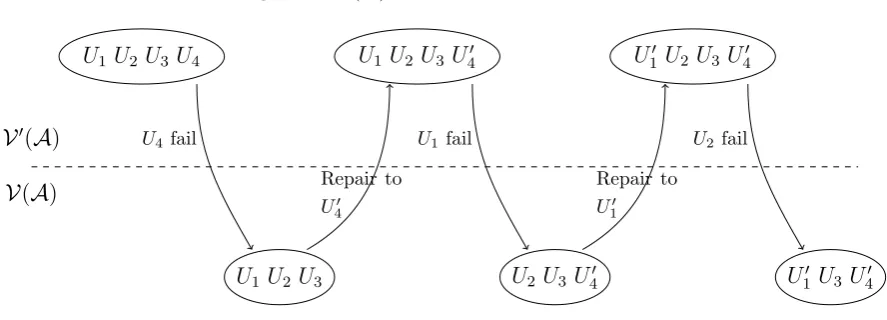
Figure 3: G(A) withn= 4, k = 3, r= 3.
U1 U2U3 U4 U1 U2 U3 U40 U10 U2 U3U40
V0(A)
V(A)
U1 U2U3 U2 U3U40 U10 U3 U40
U4fail U1fail U2fail
Repair to
U0
4
Repair to
U0
1
6
The repair condition as digraphs
We write this with m = 5, n = 4, k = 3, r = 3, α = 2 β = 1, for simplicity, but it can easily be written more generally.
We can think of the repair condition (Definition 2.2(B)) of an (m;n, k, r, α, β)-functional repair code (Σ,A) as a bipartite digraph G(A) = (V(A)∪ V0(A),E ∪ E0) as follows:
Let V(A) be a set of vertices corresponding to the sets U of 3 lines in A - each set U ∈ A is a vertex in V(A). By the repair condition, one could obtain a fourth line U0 by (r, β)-repair from any set U of 3 lines. Let V0(A) be another set of vertices corresponding to these sets U ∪ {U0},
U ∈ A, of four lines. The set of vertices of G(A) will be the (disjoint) union of these two sets of vertices.
The (directed) edges of G(Σ,A) are defined as follows: There is an edge from V = {U1, U2, U3} ∈
V(A) toV0= {U1, U2, U3, U4} ∈ V0(A) if and only ifU4 is obtain by (r, β)-repair from{U1, U2, U3}. We denote this set of edges by E. In addition, there is an edge fromV0 ={U
1, U2, U3, U4} ∈ V0(A) to V ∈ V(A) if and only if V = V0\ {U
i},i∈ {1,2,3,4}. We denote this set of edges by E0. The
set of edges ofG(A) will be the (disjoint) union of these two sets of edges.
Clearly there are edges only between V(A) and V0(A) and G(A) is a bipartite digraph. An edge from V(A) to V0(A) signifies a repair while an edge from V0(A) to V(A) signifies a node failure. Figure 3 gives a small example of what the node failures and repairs might look like.
Since each node may fail, there must be four out-edges from each vertex inV0(A), and since every three nodes must be able to repair a fourth node, there must be at least one out-edge from each vertex in V(A).
Definition 6.1. Let G = (V1∪V2, E) be a bipartite digraph with parts V1, V2. We say that G satisfies the repair condition if all vertices in V1 has outdegree at least 1 and all vertices inV2 has outdegree n.
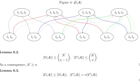
Figure 4: G(A)
l1l2 l1l3 l2 l3 l1 l4 l2 l4 l3 l4
l1 l2 l3 l1l2l4 l1 l3 l4 l2 l3l4
Lemma 6.2.
|V(A)| ≤
N
n−1
, |V0(A)| ≤
N
n
.
As a consequence, N ≥n. 2
Lemma 6.3.
|E(A)| ≥ |V(A)|, |E0(A)|=n|V0(A)|.
2
This leads to the characterisation:
Lemma 6.4. A functional repair code (Σ,A) is an exact repair code if and only if G(A) is a complete bipartite digraph (with an in-edge and and out-edge between each pair of vertices from
different parts) with |V(A)|=n, |V0(A)|= 1. 2
A functional repair code admits exact repair if it has a subgraph that satisfies the condition in Lemma 6.4, while a strictly functional repair code would satisfy the condition that there exists
V0 ∈ V0A,V ∈ V(A), such that (V0, V)∈ E0(A) but (V, V0)6∈ E(A).
We illustrate this with the strictly functional repair code of Example 3.6. Figure 4 is the digraph corresponding to the example. The dotted lines represent repairs. The node {l1, l2, l3} and the dashed lines show that if any of l1, l2 or l3 failed, they cannot be repaired from the remaining lines. And if all nodes containing l1 are removed, we have an exact repair code consisting of three non-concurrent lines.
Note that we are only encoding the repair process. We say nothing about m, q, r, k, β and
α. If a bipartite digraph satisfies the repair condition it still doesn’t say if it can be realised by any parameters. We call the digraph G realisable if there is (m, q, r, k, β, α) such that there is an (m;n, k, r, α, β)-functional repair code (FRC) (PG(m−1, q),A) withG(A)≡ G.
7
Further work
designs, since linearity is not required. This approach may be useful for functional repair code requiring repair-by-transfer ([20, 1, 22]), where the nodes contributing information for repair do not perform any computations. There has also been studies of locally repairable codes via matroid theory ([27, 28]) which may also be of interest for functional repair codes.
Construction 3.5 gives a functional repair code that is flexible in terms of locality and availability for node repairs. There are some recent work ([23]) in symbol localilty and availability: not necessarily repairing whole nodes but only some symbols in a node. It would be intresting to see how this translate into projective geometry.
The focal spread construction in Section 4 gives the only known example of a strictly functional repair code. However, it is not clear whether a generalisation to larger fields or to higher dimensions would retain this property. Indeed, it is not even clear whether one could still have a succinct description of the repair process. This indicates that there is still much to understand about this interesting structure. It is also not clear whether the distilling of the properties of functional repair from this focal spread construction into a non-recursive definition (Section 5) may be generalised. Again, this indicates that further study of this structure may be profitable.
The view of a functional repair code as a digraph allows some characterisation of exact repair codes. However, as yet it is not clear when a digraph with the right properties are actually realisable as a functional repair code. Another aspect to consider is: given a digraph, is it always possible to “complete” it so that it satisfies the repair condition or are there cases where this is impossible?
References
[1] B. S. Babu and P. Vijay Kumar. A tight lower bound on the sub-packetization level of optimal-access MSR and MDS codes. 2018 IEEE International Symposium on Information Theory (ISIT), Vail, Colorado, USA. June 2018. Available athttps://arxiv.org/abs/1710.05876.
[2] R. Bhagwan, K. Tati, Y. C. Cheng, S. Savage and G. M. Voelker. Total Recall: System support for automated availability management. In Proceedings of the 1st conference on Symposium on Networked Systems Design and Implementation (NSDI’04), Vol. 1. USENIX Association, Berkeley, CA, USA, pp. 25–25.
[3] A. G. Dimakis, P. B. Godfrey, Y. Wu, M. J. Wainwright and K. Ramchandran. Network cod-ing for distributed storage systems. IEEE Transactions on Information Theory, 56(9):4539– 4551, Sept. 2010.
[4] V. Guruswami, S. V. Lokam and S. V. M. Jayaraman. -MSR codes: Contacting fewer code blocks for exact repair. 2018 IEEE International Symposium on Information Theory (ISIT), Vail, Colorado, USA. June 2018. Available at https://arxiv.org/abs/1807.01166.
[5] J. W. P. Hirschfeld. Finite projective spaces of three dimensions. Oxford University Press. 1985.
[7] J. W. P. Hirschfeld and J. A. Thas. General galois geometries. Oxford University Press. 1991.
[8] H. D. L. Hollmann and W. Poh. Characterizations and construction methods for linear functional-repair storage codes. 2013 IEEE International Symposium on Information Theory (ISIT), Istanbul, Turkey, July 2013, pp. 336–340. Available athttp://arxiv.org/abs/1511. 02924.
[9] H. Hou and H. Li. Practical self-repairing codes for distributed storage. IEEE Asia Pacific Cloud Computing Congress (APCloudCC), Shenzhen, 2012, pp. 76–81.
[10] H. Hou, H. Li and K. W. Shum. General self-repairing codes for distributed storage systems. IEEE International Conference on Communications (ICC), Budapest, 2013, pp. 4358–4362.
[11] V. Jha and N. L. Johnson. Vector space partitions and designs. Part I - Basic Theory. Note di Matematica 29(2):165-189, 2009.
[12] F. J. MacWilliams and N. J. A. Sloane The theory of error-correcting codes. North Holland. 1983.
[13] M. Y. Nam and H. Y. Song. Binary locally repairable codes with minimum distance at least six based on partial t-spreads. IEEE Communications Letters 21(8):1683–1686, Aug. 2017. [14] F. Oggier and A. Datta. Self-repairing codes for distributed storage - A projective geometric
construction. IEEE Information Theory Workshop, Paraty, 2011, pp. 30–34.
[15] D. A. Patterson, G. Gibson and R. H. Katz. A case for Redundant Arrays of Inexpensive Disks (RAID). In Proc. ACM SIGMOD international conference on management of data, Chicago, USA, Jun. 1988, pp. 109–116.
[16] K. V. Rashmi, N. B. Shah and P. Vijay Kumar. Optimal exact-regenerating codes for dis-tributed storage at the MSR and MBR points via a product-matrix construction. IEEE Transactions on Information Theory, 57(8):5227–5239, 2011.
[17] N. Raviv and T. Etzion. Distributed storage systems based on intersecting subspace codes. 2015 IEEE International Symposium on Information Theory (ISIT), Hong Kong, 2015, pp. 1462–1466.
[18] N. Raviv, N. Silberstein and T. Etzion. Constructions of high-rate minimum storage regen-erating codes over small fields. IEEE Transactions on Information Theory, 63(4):2015–2038, April 2017.
[19] S. Sahraei and M. Gastpar. Increasing Availability in Distributed Storage Systems via Clus-tering. 2018 IEEE International Symposium on Information Theory (ISIT), Vail, Colorado, USA. June 2018. Available at https://arxiv.org/abs/1710.02653.
[21] N. Silberstein. Fractional repetition and erasure batch codes. In Coding Theory and Ap-plications, edited by R. Pinto, P. Rocha Malonek, P. Vettori. CIM Series in Mathematical Sciences, vol 3. Springer, Cham, 2015.
[22] N. Silberstein and T. Etzion. Optimal fractional repetition codes and fractional repetition batch codes. 2015 IEEE International Symposium on Information Theory, Hong Kong, 2015, pp. 2046–2050.
[23] N. Silberstein, T. Etzion and M. Schwartz. Locality and availability of array codes constructed from subspaces. 2017 IEEE International Symposium on Information Theory (ISIT), Aachen, 2017, pp. 829–833.
[24] K. Shanmugam, D. S. Papailiopoulos, A. G. Dimakis and G. Caire. A repair framework for scalar MDS codes. IEEE Journal on Selected Areas in Communications, 32(5):998–1007, May 2014.
[25] J. Sohn, B. Choi and J. Moon. A class of MSR codes for clustered distributed storage. 2018 IEEE International Symposium on Information Theory (ISIT), Vail, Colorado, USA. June 2018. Available at https://arxiv.org/abs/1801.02014.
[26] M. Vajha, B. S. Babu and P. Vijay Kumar. Explicit MSR codes with optimal access, optimal sub-packetization and small field size for d = k+ 1, k+ 2, k+ 3. 2018 IEEE International Symposium on Information Theory (ISIT), Vail, Colorado, USA. June 2018. Available at
https://arxiv.org/abs/1804.00598.
[27] T. Westerb¨ack, T. Ernvall and C. Hollanti. Almost affine locally repairable codes and matroid theory. 2014 IEEE Information Theory Workshop (ITW 2014), Hobart, TAS, 2014, pp. 621– 625.
[28] T. Westerb¨ack, R. Freij-Hollanti, T. Ernvall and C. Hollanti. On the combinatorics of locally repairable codes via matroid theory. IEEE Transactions on Information Theory, vol. 62, no. 10, pp. 5296–5315, Oct. 2016.
[29] M. Ye and A. Barg. Cooperative repair: Constructions of optimal MDS codes for all admis-sible parameters. 2018 IEEE International Symposium on Information Theory (ISIT), Vail, Colorado, USA. June 2018. Available at https://arxiv.org/abs/1801.09665.