BIROn - Birkbeck Institutional Research Online
Beckert, Walter (2019) A note on specification testing in some structural
regression models.
Working Paper.
Centre for Microdata Methods and
Practice, London, UK.
Downloaded from:
Usage Guidelines:
Please refer to usage guidelines at or alternatively
A Note on Specification Testing
in Some Structural Regression
Models
Walter Beckert
The Institute for Fiscal Studies
Department of Economics,
UCL
A Note on Specification Testing in Some Structural
Regression Models
∗
Walter Beckert
†May 10, 2019
Abstract
There exists a useful framework for jointly implementing Durbin-Wu-Hausman exogeneity and Sargan-Hansen overidentification tests, as a single artificial regression. This note sets out the framework for linear models and discusses its extension to non-linear models. It also provides an empirical example and some Monte Carlo results.
Word count: 3121.
JEL classification: C21, C26, C36.
Keywords: endogeneity, identification, testing, artificial regression.
∗I thank the editor, Debopam Bhattacharya, and two anonymous referees, for insightful comments and
suggestions that greatly improved the paper, as well as Haris Psaradakis, Ron Smith and Jouni Sohkanen for helpful comments and discussions.
†Department of Economics, Mathematics and Statistics, Birkbeck College, University of London, Malet
1
Introduction
Specification testing of structural linear simultaneous equations models with endogenous
regressors is comprehensively surveyed inHausman [1983]. A commonly applied test of the null hypothesis of exogenous regressors in linear regression models, under the maintained
assumption of the exogeneity of a set of instruments, is due toDurbin[1954],Hausman[1978],
Wu [1973]. If more instruments are available than necessary for identification, i.e. if the model is overidentified, again under the maintained assumption of the exogeneity (validity) of just identifying instruments, then a test of the validity of the imposed overidentifying
restrictions, due toSargan [1958, 1988], is another useful specification test.1
This note shows how, following a first-stage regression, in a single linear regression – on
the independent variables, the first-stage residuals and a set of candidate overidentifying
in-struments – under the maintained assumption of the validity of just identifying inin-struments,
(i) the coefficients of the structural regression equation can be consistently estimated, (ii)
the null hypothesis of exogenous regressors can be tested and, in an overidentied model, (iii)
the null hypothesis of the validity of overidentifying restrictions can be tested as well.
Importantly, the analysis of the linear regression model is interesting because the insights gained from it carry over to nonlinear models, such as nonlinear regression models and
Generalized Linear Models [McCullagh and Nelder, 1983] in which there typically exist a variety of definitions for residuals – including Pearson, Anscombe, deviance residuals – and
it is not a priori clear which one to use as the basis to construct test statistics and measure of
fit. Such models can be estimated using an artificial or Gauss-Newton regression [Davidson and MacKinnon, 1990, 1993, 2001], and this algorithm provides the conceptual link to the analysis within the linear regression framework.
While the idea is straightforward it does not appear to be discussed in the literature,
so I hope that this paper can assist practitioners, by alerting them to a tool that can be
implemented easily and usefully in a variety of widely applied regression models.
2
Linear Model
2.1
Specification Testing
Consider the linear regression model
y=X1β1 +X2β2+, (1)
where y is an N × 1 vector, X1 and X2 are N × n1 and N ×n2 matrices of regressors
with full column rank, withβ1 and β2 being commensuraten1- and n2-vectors of regression
coefficients, and an N-vector of disturbances satisfying E[X02] = 0 and E[X01] 6= 0, i.e. the regressors X1 are endogenous.
Also, suppose thatZis anN×mmatrix of instruments forX1, withm > n1, full rankm,
and E[Z0(I−PX2)X1] having full rank n1, where PX2 =X2(X
0
2X2)−1X02. i.e. the order and rank conditions for identification of equation (1) are satisfied.2 The maintained assumption is that a subset of n1 columns of Z is uncorrelated with the structural regression errors
. Furthermore, it is assumed that the elements of are mean zero and homoskedastic,
conditional on X and Z. The case of conditionally heteroskedastic errors is discussed in section 2.4 below.
Let X = [X1,X2] denote the N ×(n1 +n2) matrix of regressors, and W = [X2,Z] the
N×(n2+m) matrix of instruments. Also, letPW =W(W’W)−1W0. For ˆX1 =PWX1 the
fitted values of the first-stage regressions,
y = Xˆ1β1+X2β2+
X1−Xˆ1
β1+ (2)
= Xˆβ+ (I−PW)X1β1+ (3)
= Xˆβˆ2SLS + ˆX
β−βˆ2SLS
+ (I−PW)X1β1+ (4)
where ˆX = [ ˆX1,X2] = PWX and ˆβ2SLS denotes the two-stage least squares estimator for
β0 = [β10, β20].
We follow the interpretation of Stock [2015] that, under the maintained assumption that at leastn1 valid instruments are available, one can test the null hypothesis of all instruments being valid, i.e. of the model being overidentified, against the alternative that up tom−n1
instruments are invalid. Define the second-stage regression residuals
ˆ
= y−Xˆβˆ2SLS (5)
= Xˆ β−βˆ2SLS
+ (I−PW)X1β1+, (6)
and notice that
ˆ
= −Xˆ (X0PWX) −1
X0PW+ (I−PW)X1β1+ (7)
= I−PWX(X0PWX) −1
X0PW
+ (I−PW)X1β1. (8)
2The relevance condition implies that, in the reduced form system forX
1,X1=X2Π1+ZΠ2+u, Π2 is
identified, Π2= E[Z0(I−PX2)Z]
−1
Therefore, a version of the Sargan test of the validity of the overidentifying restrictions in
this model is based on the test statistic
SN = ˆ0PWˆ (9)
= 0PW −PWX(X0PWX) −1
X0PW
. (10)
Since the rank of the central matrix is equal to its trace, and its trace is equal to m−n1,
under the null hypothesis the statistic SN is asymptotically distributed σ2χ2m−n1, where σ
2
is the conditional variance of the regression errors .
The Durbin-Wu-Hausman test examines the null hypothesis of the exogeneity of the
regressorsX1, against the alternative that these regressors are correlated with the regression error term. It is based on the OLS estimator of then1-vector γ in the regression
y=X1β1+X2β2+ ˆUγ+ν, (11)
where ˆU = (I−PW)X1 are the residuals of the first-stage regressions, or so-called control
functions. This regression can be interpreted as an “artificial regression” in the sense of
Davidson and MacKinnon[1990,1993,2001]3 because under the null hypothesis of exogeneity the coefficient vector on the control functions γ = 0.4 The Durbin-Wu-Hausman test
therefore rejects the null hypothesis of exogeneity when ˆγ is statistically significant. It
is well known that the OLS estimator of β in this regression is identical to the two-stage
least squares estimator ˆβ2SLS.
Now consider the expanded artificial regression
y = X1β1+X2β2+ ¯Zδ+ ˆUγ+ξ (12)
= Xβ+ ¯Zδ+ ˆUγ+ξ, (13)
where ¯Z is an arbitrary subset of m−n1 columns of Z. Under the null hypothesis that all
overidentifying restrictions are valid, the m−n1-vector δ = 0. And if and only if the null hypothesis is true, the OLS estimator of β is equal to the two-stage least squares estimator
and the OLS estimator of γ permits a Durbin-Wu-Hausman exogeneity test.5 Incidentally,
3SeeDavidson and MacKinnon [1993], chapters 3.6 and 6. 4This can be seen from the reduced form systemX
1 =X2Π1+ZΠ2+u,EX0u=0andE[Z0u] =0,
so thatX1is correlated withif, and only if,EX01|X,Z
=E
Π01X02+ Π02Z0+u0|X,Z
=E[0u|X,Z] =
γ06=00 a.s.
5Analogous to the argument related to (11), this follows from the reduced form forX
1, orthogonality
these considerations show that the exogeneity test is not independent of the validity of all
the instruments used to implement the test.
Since ˆU is orthogonal toW,
PWy= ˆXβ+ ¯Zδ+PWξ. (14)
Here, PWξ, captures the exogenous part of the disturbances under the hypothesis that all
instruments are valid. Define PXˆ = ˆX
ˆ
X0Xˆ
−1 ˆ
X0. Then,
ˆ
δ = δ+Z¯0(I−PXˆ) ¯Z
−1
¯
Z0(I−PXˆ)PWξ (15)
= δ+Z¯0I−PWX(X0PWX) −1
X0PW
¯
Z
−1
× Z¯0
I−PWX(X0PWX) −1
X0PW
PWξ. (16)
Therefore, under the null hypothesis, the statistic
˜
SN = ˆδ0
¯
Z0I−PWX(X0PWX) −1
X0PW
¯
Zδˆ (17)
= ξ0PW −PWX(X0PWX) −1
X0PW
ξ (18)
has a σ2
ξχ2m−n1 distribution and thus ˜SN/σˆ
2
ξ is equivalent to the test statistic SN/σˆ2, where
ˆ
σ2 denotes the squared standard error of the respective regression.6
Hence, the expanded artificial regression (13) implements the Durbin-Wu-Hausman ex-ogeneity and Sargan overidentification tests as a single regression. In this regression, the
null hypothesis that this paper focusses on is that δ =0, given that the hypothesis γ = 0
is rejected. As the Monte Carlo simulations in subsection 2.3 show, the first test does not significantly affect the size or power of the second test.
2.2
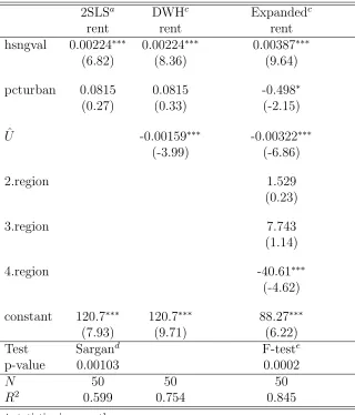
An Empirical Illustration
Table 1 provides an empirical example. It uses data provided by the statistical software Stata
for the purpose of illustrating the Sargan test.7 For the fifty US states, the data comprises
rental rates for apartments (rent), next to housing values (hsngval) and the percentage of the
state’s population living in urban areas (pcturban). The housing values regressor is treated
6The test of the null hypothesis thatδ=0is typically implemented as anF
m−n1,N−(n2+m+1) test. For
largeN, the squared standard error of the regression ˆσ2
ξ converges in probability toσ
2
ξ, so that thisF-test
is asymptotically equivalent to aχ2
m−n1 test.
as potentially endogenous in the regression of rents on housing values and the percentage of
urban population at the state level. Median family income and 3 regional dummies - for the
state’s central, southern and western areas - are considered as instruments so that there are
three over-identifying restrictions. The example shows that both the Sargan test and the
test of the joint significance of ¯Z, the three regional dummies, reject the null hypothesis of
the validity of the over-identifying restrictions.
2.3
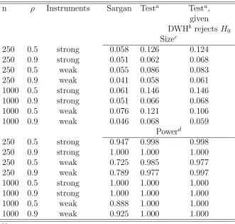
Monte Carlo Simulation
The design of the Monte Carlo study follows Hahn and Hausman [2002] and Lee and Okui
[2009]. The data is generated as
y1i = βz0iπ+z 0
iγ+v1i
y2i = z0iπ+v2i, i= 1,· · · , n
where
zi i.i.d.
∼ N(0,IK), K = 5
v1i
v2i
!
i.i.d.
∼ N
0
0
! ,
"
1 ρ
ρ 1
#! .
Here, πk = φ, k = 1,· · · , K, and φ is chosen such that the theoretical R2 of the first-stage
regression, R2 = KφKφ2+12 , equals 0.01 and 0.2, respectively; these two cases capture situations
with weak and strong instruments, respectively.8 The parameter ρ is set to 0.5 and 0.9, to simulate cases of moderate and strong endogeneity. The parameter β is set such that the
errors in the structural equation y1i =βy2i+i, i.e. i =v1i−βv2i, have unit variance. We
investigate the size of specification tests when γ = 0, and their power when γ1 = 0.1 and
γk = 0, k = 2,· · · , K. We run 2000 simulations, for sample sizes of n= 250 and n = 1000.
Table 2 summarises the results of our simulations. The size of the proposed test is
generally slightly larger than the size of the conventional Sargan test, although the difference
diminishes the stronger the simulated endogeneity is. The power of the proposed test, on
the other hand, exceeds the one of the conventional Sargan test.9 The results also show that
both, the size and power of the proposed test, do not hinge on this being a second-stage test,
following a first-stage Durbin-Wu-Hausman exogeneity test.
8The values ofφare 0.04495 and 0.22361.
9The reason for the strong power is that in the simulations the additional instruments ¯Zimprove the fit
2.4
Extension to Heteroskedastic Models
Davidson et al. [1985] and Wooldridge [1995] discuss diagnostic tests based on the score or Lagrange multiplier principle that are heteroskedasticity robust.10 Their approach can be
adapted to the test proposed in this paper.
Let ˆν denote the residuals of the regression (11). Note that this regression equation is simply (13), subject to the restriction that δ = 0, i.e. subject to the null hypothesis of valid overidentifying restrictions. And define ˆRas theN×(n2+m) matrix of residuals of the
regres-sion of ¯Zonto [X,Uˆ]. Then, regress ann-vector of ones onto ˆν·Rˆ = [ˆνiRˆik]i=1,···,n;k=1,···,n2+m,
without intercept, and retrieve the sum of squared residuals, SSR. Then, the test statistic
N−SSR is distributedχ2
m−n1 under the null hypothesis that the overidentifying restrictions
are valid. Appendix A provides a formal derivation.
3
Extension to Nonlinear Models
A nonlinear version of model (1) is given by
y=x(β) +, (19)
where x(·) is a known, differentiable function of β ∈ Rn1+n2. This function is the inverse
link function in the class of Generalized Linear Models discussed in McCullagh and Nelder
[1983] who also propose an estimation algorithm which amounts to an iterative weighted least squares procedure, a variant of the Newton-Raphson algorithm.
Endogeneity in the nonlinear model amounts to n1 elements of E[∇βx(β)0] being
non-zero.11
Davidson and MacKinnon [1990, 1993, 2001] have shown how an “artificial regression”, or Gauss-Newton regression, can be used to test the null hypothesis of exogeneity, i.e.
the consistency of the nonlinear least squares (NLS) estimator ˆβ, under the maintained
hypothesis of a set of valid instruments Z.
The NLS estimator solves
Xβˆ
0
y−xβˆ =0, (20)
where X(β) = ∇βx(β) is assumed to have full column rank in a neighborhood about the
10Wooldridge [2010] discusses a heteroskedastic robust version of the Durbin-Wu-Hausman test and the
Sargan test as in9. See also Windmeijer et al.[2018] andChao et al. [2014].
11This can be thought of as β0 = (β0
1, β02), where β1 ∈Rn1 andβ
2 ∈Rn2, andX
1 =∇β1x(β) satisfying
true population β.
As an analogue to the residual based exogeneity test in the linear model as implemented
in (11),Davidson and MacKinnon [1993] propose the test of the null hypothesis ofτ =0in the regression
y−xβˆ=Xβˆα+ (I−PW)X∗
ˆ
βτ+ζ, (21)
whereX∗ are them−n1-columns ofX that are not annihilated by the orthogonal projector
(I − PW) and W = [X2,Z] is a set of m+n2 instruments.12 The contribution of (I −
PW)X∗
ˆ
βcan again be viewed as a set of control functions. This is an artificial or
Gauss-Newton regression because under the null hypothesis one would expect the least squares
estimator of τ to be statistically insignificant.13 The regressand in this Gauss-Newton regression is ˆ=y−xβˆ.
Now consider the instrumental variable estimator ˜β which satisfies
Xβ˜
0
PW
y−xβ˜=0. (22)
The residuals induced by the IV estimator are ˜=y−xβ˜. The Sargan test of the validity
of over-identifying restrictions is14
TN = ˜0PW˜ (23)
≈ y−x(β)−X(β)β˜−β
0
PW
y−x(β)−X(β)β˜−β (24)
=
I−X(β)
Xβ˜
0
PWX
˜
β −1
Xβ˜
0 PW ! !0 PW ×
I−X(β)
Xβ˜
0
PWX
˜
β −1
Xβ˜
0 PW ! ! (25)
= 0 PW −PWX(β)
Xβ˜
0
PWX
˜
β −1
Xβ˜
0
PW
!
. (26)
Under the null hypothesis, ˜β is consistent forβ, and providedX(·) is continuous,X( ˜β) tends
toX(β) in large samples. Then, under the null hypothesis,TN is asymptotically distributed
χ2
m−n1.
12Here,X
2=∇β2x(β), satisfyingE[X02] =0. 13As in the linear case, the reduced form for X
1 =∇β1x(β) =∇β2x(β)Π1+ZΠ2+u, E[∇β1x(β)0] =0
andE[Z0] =0, implies∇β1x(β) is endogenous if, and only if, E[0u|X(β),Z] =τ06=00.
14In the approximation following the definition ofT
Now consider an expanded Gauss-Newton regression, ˆ =X ˆ β
α+ ¯Zπ+ (I−PW)X∗
ˆ
β
τ +ζ, (27)
where ¯Z is an arbitrary subset of m − n1 columns of Z. Under the null hypothesis of
exogeneity, just as in (13), one would expect the least squares estimates ˆτ to be statistically insignificant.15 Also, analogous to (13), since
PWˆ=PWX
ˆ
β+ ¯Zπ+PWζ, (28)
it follows that
ˆ
π = π+ Z¯0 I −PWX
ˆ
β
Xβˆ
0
PWX
ˆ
β −1
Xβˆ
0
PW
!
¯
Z
!−1
×Z¯0 I−PWX
ˆ
β
Xβˆ
0
PWX
ˆ
β −1
Xβˆ
0
PW
!
ζ, (29)
a test statistic based on ˆπ satisfies
˜
TN = ˆπ0 Z¯ 0
I−PWX
ˆ
β
Xβˆ
0
PWX
ˆ
β −1
Xβˆ
0 PW ! ¯ Z ! ˆ π (30)
= ζ0 PW −PWX
ˆ
β
Xβˆ
0
PWX
ˆ
β −1
Xβˆ
0
PW
!
ζ. (31)
Under the null hypothesis, ˆβ is consistent for β, and ˜TN is distributed asymptotically
σ2
ζχ2m−n1.
Hence, again, the expanded artificial regression implements the exogeneity and
overiden-tification test is a single regression.
4
Conclusions
This note presents a useful but not widely known framework for jointly implementing
Durbin-Wu-Hausam exogeneity and Sargan-Hansen overidentification tests, as a single artificial
regression. It covers linear models and discusses its extension to a class of non-linear models. Future research might explore how to adapt this methodology to semi-parametric single
index models [Horowitz,2009] and quantile regression models in which the control function
15Given the orthogonality of ¯Z and u in the reduced form system, under the null hypothesis,
approach is already widely employed [Blundell and Powell, 2004, Lee,2007].
References
Richard W. Blundell and James L. Powell. Endogeneity in Semiparametric Binary Response
Models. The Review of Economics Studies, 71(3):655–679, 2004.
John C Chao, Jerry A Hausman, Whitney K Newey, Norman R Swanson, and Tiemen
Woutersen. Testing overidentifying restrictions with many instruments and heteroskedas-ticity. Journal of econometrics, 178:15–21, 2014.
Russell Davidson and James G. MacKinnon. Specification Tests Based on Artificial
Regressions. Journal of the American Statistical Association, 85(409):220–227, 1990.
Russell Davidson and James G. MacKinnon. Estimation and Inference in Econometrics.
Oxford University Press, 1993.
Russell Davidson and James G. MacKinnon. Artificial Regressions. Queen’s Economics
Department Working Paper No. 1038,, 2001.
Russell Davidson, James G MacKinnon, and Russel Davidson. Heteroskedasticity-robust
tests in regressions directions. InAnnales de l’INSEE, pages 183–218. JSTOR, 1985.
James Durbin. Errors in Variables. Review of the International Statistical Institute, 22(1/3):
23–32, 1954.
Jinyong Hahn and Jerry Hausman. A new specification test for the validity of instrumental
variables. Econometrica, 70(1):163–189, 2002.
Lars P. Hansen. Large Sample Properties of Generalized Method of Moments Estimators.
1982.
Jerry A. Hausman. Specification Tests in Econometrics. Econometrica, 46(6):1251–1271,
1978.
Jerry A. Hausman. Handbook of Econometrics, Vol.1, chapter Specification and estimation
of simultaneous equation models, pages 391–448. North Holland, 1983.
Joel Horowitz. Semiparametric and Nonparametric Methods in Econometrics. Springer
Sokbae Lee. Endogeneity in quantile regression models: A control function approach.Journal
of Econometrics, 141(2):1131–1158, 2007.
Yoonseok Lee and Ryo Okui. A specification test for instrumental variables regression with
many instruments. 2009.
P. McCullagh and J.A. Nelder. Generalized Linear Models. Chapman and Hall, 1983.
John D. Sargan. The Estimation of Economic Relationships Using Instrumental Variables.
Econometrica, 26(3):393–415, 1958.
John D. Sargan. Contributions to Econometrics: John Denis Sargan, vol. I, chapter
Testing for misspecification after estimating using instrumental variables, pages 213–235.
Cambridge University Press, 1988.
James H Stock. Instrumental variables in statistics and econometrics. 2015.
Halbert White et al. A heteroskedasticity-consistent covariance matrix estimator and a direct
test for heteroskedasticity. econometrica, 48(4):817–838, 1980.
Frank Windmeijer et al. Testing over-and underidentification in linear models, with
applications to dynamic panel data and asset-pricing models. University of Bristol Department of Economics Working Paper, 2018.
Jeffrey M Wooldridge. Score diagnostics for linear models estimated by two stage least
squares. Advances in econometrics and quantitative economics: Essays in honor of
Professor CR Rao, pages 66–87, 1995.
Jeffrey M Wooldridge. Econometric analysis of cross section and panel data. MIT press,
2010.
De-Min Wu. Alternative Tests of Independence between Stochastic Regressors and
A
Heteroskedasticity Robust Test
Assume the errors in (13) are i.i.d. normal, with mean zero and heteroskedastic variances, conditional on X and Z.16 Then, under the null hypothesis δ= 0,
y0(I−PX,Uˆ) ¯Z=ν0(I−PX,Uˆ) ¯Z, (32)
with mean zero and variance-covariance matrix ¯Z0(I−PX,Uˆ)Ω(I−PX,Uˆ) ¯Z, where Ω is a
diagonal matrix when the errors are conditionally heteroskedastic. Therefore, under the
assumption of normality, the statistic
L=y0(I−PX,Uˆ) ¯Z
h
¯
Z0(I−PX,Uˆ)Ω(I−PX,Uˆ) ¯Z
i−1
¯
Z0(I−PX,Uˆ)y (33)
is distributed χ2
m−n1. Using results in Davidson et al. [1985] and White et al. [1980], it can
be implemented by replacing Ω with ˆΩ = diag(ˆνi), where ˆν is the vector of residuals of
regression (11). Let ˆLdenote this feasible test statistic.
Now consider the regression of an n-vector of ones onto ˆν·Rˆ. Notice, first, that
ˆ
ν·Rˆ = diag(ˆνi)(I−PX,Uˆ) ¯Z (34)
= νˆ0(I−PX,Uˆ) ¯Z (35)
= y0(I−PX,Uˆ) ¯Z (36)
Therefore, the resulting sum of squared residuals is
SSR = N −νˆ0(I−PX,Uˆ) ¯Z
h
¯
Z0(I−PX,Uˆ)diag(ˆνi)(I−PX,Uˆ) ¯Z
i−1
¯
Z0(I−PX,Uˆ)ˆν (37)
= N −y0(I−PX,Uˆ) ¯Z
h
¯
Z0(I−PX,Uˆ)diag(ˆνi)(I−PX,Uˆ) ¯Z
i−1
¯
Z0(I−PX,Uˆ)y (38)
= N −L.ˆ (39)
Therefore, ˆL=N −SSR.
B
Tables
16Absent the assumption of normality, the derivation of the distribution of the test statistic holds
Table 1: Example
2SLSa DWHc Expandedc
rent rent rent
hsngval 0.00224∗∗∗ 0.00224∗∗∗ 0.00387∗∗∗
(6.82) (8.36) (9.64)
pcturban 0.0815 0.0815 -0.498∗
(0.27) (0.33) (-2.15)
ˆ
U -0.00159∗∗∗ -0.00322∗∗∗
(-3.99) (-6.86)
2.region 1.529
(0.23)
3.region 7.743
(1.14)
4.region -40.61∗∗∗
(-4.62)
constant 120.7∗∗∗ 120.7∗∗∗ 88.27∗∗∗
(7.93) (9.71) (6.22)
Test Sargand F-teste
p-value 0.00103 0.0002
N 50 50 50
R2 0.599 0.754 0.845
t statistics in parentheses
∗ p <0.05,∗∗ p <0.01,∗∗∗ p <0.001
Notes:
a 2SLS: hsngval instrumented by family income and 3 region dummies. b Durbin-Wu-Hausman regression.
c Expanded artificial regression, as in equations (12) and (13). d The Sargan test statistic has aχ2
3distribution.
eThe test statistic has anF
Table 2: Monte Carlo Simulations
n ρ Instruments Sargan Testa Testa,
given DWHb rejects H
0 Sizec
250 0.5 strong 0.058 0.126 0.124
250 0.9 strong 0.051 0.062 0.068
250 0.5 weak 0.055 0.086 0.083
250 0.9 weak 0.041 0.058 0.061
1000 0.5 strong 0.061 0.146 0.146
1000 0.9 strong 0.051 0.066 0.068
1000 0.5 weak 0.076 0.121 0.106
1000 0.9 weak 0.046 0.068 0.059
Powerd
250 0.5 strong 0.947 0.998 0.998
250 0.9 strong 1.000 1.000 1.000
250 0.5 weak 0.725 0.985 0.977
250 0.9 weak 0.789 0.977 0.997
1000 0.5 strong 1.000 1.000 1.000
1000 0.9 strong 1.000 1.000 1.000
1000 0.5 weak 0.888 1.000 1.000
1000 0.9 weak 0.925 1.000 1.000
Notes:
2000 Simulation sample draws. The nominal size of all tests is 0.05.
a Proposed test of null hypothesis thatδ= 0.
b Durbin-Wu-Hausman regression based exogeneity test. c Here, γ=0.
d Here,γ