Reliability Analysis in Component Based Software Systems

(1)

International Journal of Emerging Technology and Advanced Engineering

Website: www.ijetae.com (ISSN 2250-2459, ISO 9001:2008 Certified Journal, Volume 7, Issue 9, September 2017)

Reliability Analysis in Component Based Software Systems

Bishwajeet Kumar

1

, Dr. I. B. Lal

2

1_{Research Scholar, B.R.A.Bihar University, Muzaffarpur, Bihar, India}

2_{Assistant Professor, Deptt. of Information Technology, L.N. Mishra College of Business Management, Muzaffarpur, India} Abstract: Component-Based Software Systems are

composed by assembling components already developed and prepared for integration. The components are basic unit in Component Based Development (CBD). It is an independent unit of composition which can execute in itself and can be deployed independently, also it can be defined as a physical 'package', which can be plugged into a system without internal modification. An erroneous component might infect other components, leading to failure of the entire system. The reliability of a whole program or software is influenced by reliability estimates for its components. Hence, the reliability of such systems is estimated using the reliability of the individual components and their interconnection mechanism. It is reasonable to that a well tested individual component is reliable and, performs its intended functionality at individual level, but when interconnected with other components may behave unreliably. Hence, now–a–days, software developers are more interested to use software components for rapid application development through reusability and to meet new and frequently changing requirements of the customers/users. The challenge for software developers is to deliver/maintain the quality of the product and thus the reliability of the software. The authors have attempted to study and present an analysis on the component based software system reliability.

Keywords: Software reliability, Components based software, fault, failure, functional analysis, path propagation probability, component architecture graph.

I. INTRODUCTION

Computer system plays more and more important role in our daily lives as computer system failures can lead to a huge economic loss or even endanger human life. Reliability is one of the most important quality requirements of computer systems. A computer system comprises two major components, hardware and software. The growing importance of software dictates that the software reliability is the major stumbling block in highly dependable computer system. Researchers have focused on procedural and object oriented software reliability.

Till the advent of component based software engineering, the approach of software development was procedural which had been quite problematic for the software developers. Some of the problems related with the procedural approach could be enlisted as follows:-

 Problem of debugging

 High memory requirement

 High coupling and thus high complexity

 Problem of management in change and

maintenance

 Increased operational cost

 Problems and version control

 High execution time

 High effort requirement

 Low productivity

 High total development time

 Failed to meet frequently changing requirements, as of today,

 Difficulties in integrating the software,

 Problems of reliability with a long procedural programs, etc.

Keeping in view such problems, software product was also compared with the general hardware products which are constituted, by the number of components, where each component is manufactured independently with quality consciousness, ensuring the good quality of each component. The computer scientists also had in their mind why not software be also considered to be a product like hardware consisting of number of components, where each module or small programs be considered as a component. With this approach of software development, the quality of each component could be considered independently, ensuring the overall quality of the software product. The reliability problems with the procedural software could be reduced and overcome with this component based software development approach.

(2)

International Journal of Emerging Technology and Advanced Engineering

Hence, now–a–days, software developers are more interested to use software components for rapid application development through reusability and to meet new and frequently changing requirements of the customers/users. The challenge for software developers is to deliver/maintain the quality of the product and thus the reliability of the software.

In a component - based system reliability is estimated using the reliability of the individual components and their inter-connection mechanisms. In the foregoing discussions we would attempt to find that reliability of an overall Component based Software System is also affected by error propagation probabilities and path propagation probabilities.

In a Component based software, a component might be functioning independently well but when integrated with other components might produce errors and might not function properly. Hence, it is reasonable to consider that composite system will be reliable but components, which were tested alone in isolation for their reliability, might behave unreliably, when connected to other components. Besides, some component behaviours can be non-functional and do not manifest themselves until after the composition. Such behaviours can undermine the reliability of the software. Furthermore, a component which is reliable, when connected to a composition is simply the erroneous component, although highly reliable, the resulting composed system will be erroneous and useless. In these software systems, the reliability of the software is also highly concerned with the paths established, transition paths with branching, constructs, loops, and various other factors like usage ratio, sensitivity and component impact, besides the component itself and its interfaces with other components

II. COMPONENTS BASED SOFTWARE ENGINEERING

Component-based software engineering (CBSE) emerged in the late 1990s as a reuse-based approach to software systems development and it is becoming increasingly popular. Its creation was motivated by designer's frustration that objects oriented development had not led to extensive reuse, as originally suggested. Single object classes were too detailed and specific, and often had to be found with an application at compile time1. Clements [95] describes CBSE in the following way:

"CBSE embodies the "buy, don't build" philosophy espoused by Fred Brooks and other. In the same way that early subroutines liberated the programmer from thinking about details, [CBSE] shifts the emphasis from programming software to composing software systems. Implementation has given way to integration as the focus".

CBSE is the process of defining, implementing and integrating or composing loosely coupled independent components into systems. It has become an important software development approach because software systems are becoming larger and more complex and customers are demanding more dependable software that is developed more quickly. The only way that we can cope with complexity and deliver better software more quickly is to reuse than re-implement software components.

The reuse-oriented approach of software component relies on a large base of reusable software components and some interesting framework for these components. Sometimes, these components are systems in their own right (COTS) or commercial off-the shelf systems) that may provide specific functionality such as text formatting or numeric calculation. The component-based model leads to software reuse, and reusability provides software engineers with a number of measurable benefits. Based on studies of reusability, QSM Associates, Inc. reports component-based leads to a 70% reduction in development cycle time, an 84% reduction in project cost, and a productivity index of 26.2, compared to an industry norm of 16.92.

Modern software systems become more and more large-scale, complex and uneasily controlled, resulting in high development cost, low productivity, unmanageable software quality and high risk to move to new technology. Consequently, there is a growing demand of searching for a new, efficient, and cost-effective software development paradigm. The component-based software development approach is one of the most promising solution today.

(3)

International Journal of Emerging Technology and Advanced Engineering

III. COMPONENT BASED SOFTWARE SYSTEM RELIABILITY

ANALYSIS

In this paper, we present a number of methods for software reliability analysis which can be useful for reliability estimation for a component based software system:-

1. Failure modes, affects, and criticality analysis (FMECA):- This method is used to identify the potential failure modes of each of the functional block (Component) as a system, and to study the effects of these failures.

2. Fault tree analysis: - The fault tree is a tree structure of all possible combinations of potential failures and events that cause system failures. The construction of a fault tree starts with the specified system failure and then with the cause of this failure. Hence, its construction is a deductive approach. Failures and events are combined in binary approach through logic gates, which can be quantitatively assessed/ evaluated.

3. Cause and effect diagrams: - These diagrams are frequently and dominantly used by quality engineers to assess the possible causes of quality related problems, which can be also used by software engineers in reliability engineering to find the potential causes of system failures.

4. Bayesian belief networks: - It can be used by software engineers to identify and illustrate potential causes for system failures. Bayesian belief networks are more flexible than fault -tree because it does not require binary representation. In this network, probability distributions may be evaluated quantitatively by a Bayesian approach. A Bayesian belief network (BBN) can be used as an alternative to fault tree and cause and effect diagrams to illustrate the relationships between a system failure and its causes and contributing factors. A BBN is more general than a fault tree since the causes do not have to be binary events. It is a directed acyclic graph.

5. Event tree analysis: - It is an inductive technique where we start with a system deviation and then try to identify how this deviation may develop. The possible events following the deviation will usually be a function of various barriers and constraints that are designed into the system when we have access to probability estimates for the various barriers, we may carry out quantitative analysis of the event tree.

6. Reliability Block Diagram (RBD):- To ensure that the system function is fulfilled, the functioning of each functional block/ component is a matter of concern regarding the reliability of the system. To illustrate this, we can construct reliability block diagram. It is a success oriented network diagram the structure of which is mathematically described by structure functions.

Regarding the reliability of a software system, the system may generally be considered from two different points of view:-

1. Structural Aspect: - It is concerned with the structure of modules and their interconnections.

2. Functional Aspect:-It is concerned with the various functions of the system and subsystems/components and how functions are fulfilled.

IV. FUNCTIONAL ANALYSIS

A 'function' is an intended effect of a functional block and should be defined such that each function has a single definite purpose. Every function be named and have a declarative statement or structure. It should say 'what' is to be done rather than 'how'. A functional requirement is a specification of the performance criteria related to a function.

To identify all potential failures, the reliability engineer must have a thorough and clear understanding of the various functions of each functional block of component or module.

The objective of functional analysis is to:-

1. Identify all the functions of the system,

2. Identify the functions required in the various operational modes,

3. Provide a hierarchical decomposition of system functions,

4. Describe how each function is realized,

5. Identify the interrelationships between functions 6. Identify interfaces with modules, other systems and

with the environment.

Classification of Functions:-

A classification of functions is highly required for the purpose of identification and analysis regarding performance and reliability of components and the system as a whole. One possible classification may be as follows:-

1. Essential Function: - These are the functions required to fulfill the intended purpose for which the component has been built.

2. Auxiliary Function: - These functions are supposed to support the essential functions. Failure of auxiliary function may be more critical in some cases.

(4)

International Journal of Emerging Technology and Advanced Engineering

Website: www.ijetae.com (ISSN 2250-2459, ISO 9001:2008 Certified Journal, Volume 7, Issue 9, September 2017) 4. Information Functions: - These functions are concerned

with message passing, condition monitoring, control bits, and so forth.

5. Interface Functions: - These functions apply to the interfaces between the functional blocks or components or modules in question and other functional blocks or modules.

6. Superfluous Functions: - Some functional blocks or components may have functions that are never used. These are the results of iterative modifications in the system. It may also be the case when the functional block has been designed for an operational context that is different from the actual operational context. The failure of superfluous functions may cause failure to other functions which might affect the reliability.

V. FAILURES AND FAILURE ANALYSIS

Failure: - A failure is the eventwhen a required function is terminated (exceeding the acceptable limits).

Fault: - It is the state of an item characterized by inability to perform a required function. It is a state resulting from a failure.

Error: - It is discrepancy between a computed, observed or measured value or condition and the true, specified or theoretically correct value or condition. An error is (yet) not a failure because it is within the acceptable limits of deviation from the desired performance (target value).

Failure Modes:- It is important to realize that a failure mode is manifestation of failure as seen from the outside that is, the termination of one or more functions.

As a point of reliability consideration, the Reliability Engineer is required to know the failure modes, which is a description of a fault, that is, how a fault is observed. To identify the failure modes it is necessary to study the output of the various functions. Some function may have several outputs. It is necessary to determine whether the output requirements are fulfilled or not. In some cases, the output may be specified as a target value with an expectable derivation.

The software failures may be classified as:-

1. Intermittent failures: - Failure that occur only for a very short period.

2. Complete failure: - It causes complete lack of a required function.

3. Partial failure: - Failures that leads to a lack of some function but don't cause a complete block of required function.

4.Sudden failures: - Failures that could not be forecast by examination or testing, which might be due to hardware failures, operating system malfunctioning and memory overload.

5. Gradual failures: - Failures that could be forecast by testing or examination. It can be recognized by comparing actual performance with the specified performance.

6.Catastrophic failures: - A failure which is complete and sudden.

7. Degraded failures:- This failure is both partial and gradual. It is some kind of wear - out situation, which is not due to software failure, but for other reasons, such as hardware malfunctioning or technological obsolescence.

For all such kind of failures, repair action is required to return the functional block to a functioning state.

Failure Causes and Failure Effects: - A system is decomposed into subsystems and ultimately to modules and components in hierarchical fashion. Failure mode at one level in the hierarchy will often be caused by failure modes on the next lower level. It is important to link failure modes on lower levels to the main top level, in order to provide traceability to the essential system responses as the functional structure is returned.

Failure causes is the situation arose during design, development or use (Software Operation), which results into failure. It is necessary information required to avoid failures or reoccurrence of failures.

The failure causes may be classified as:-

1. Design failure: - This is due to incorrect or inadequate design of functional block, component, or module and their interfaces.

2. Misuse failure: - It is due to the application of stresses during use that exceed the stated capabilities of the functional block.

3. Mishandling failure: - It is caused by incorrect handling.

4. Ageing failure: - A failure whose probability of occurrence increases with the passage of time, as a result of processes in the functional block.

5. Development failure:- A failure due to non- conformity during development to design of a functional block or processes.

VI. FAILURE MODES,EFFECTS AND

CRITICALITYANALYSIS

(5)

International Journal of Emerging Technology and Advanced Engineering

It has been one of the first systematic techniques for failure analysis so as to maintain and enhance the reliability, which was developed by reliability engineers in 1950s for military systems. It involves reviewing as many component, assembles, and subsystems as possible to identify failure modes, its causes and effects of such failure. An FMEA becomes a failure mode, effects and criticality analysis (FMECA), if criticalities or priorities are assigned to the failure mode effects.

According to IEEE std. 352, the objectives of FMECA are to:-

1.Assist in selecting design alternatives with high reliability and high safety potential during the early design phase.

2.Ensure that all conceivable failure modes and their effects on operational success of the system have been considered.

3.List potential failures and identify the magnitude of their effects.

4.Develop early criteria for test planning and the design of the test.

5.Provide a basis for quantitative reliability and availability analysis.

6.Provide historical documentation for future reference to aid in analysis of failures and consideration for design changes.

7.Provide input data for trade off studies 8.Provide basis for corrective action priorities.

An FMECA is mainly a quantitative analysis and should be carried out by the designers during the design phase of a system. The purpose is to identify design areas where improvements are needed to meet reliability requirements. It is an important basis for design reviews and inspections. FMECA should be integrated into the software product development process from early concept phase and be updated in later development phases and in operational phase.

VII. FAULT TREE ANALYSIS

It is a very important technique for risk and reliability studies. This technique was first introduced at Bell telephone Laboratories in 1962, whereas, the Boeing Company improved the technique by introducing computer programs for both qualitative and quantitative, fault free analysis. It is a logic diagram that displays the interrelationships between a potential critical event and causes for this event. Possible results from the analysis may be:-

A listing of the possible combinations of environmental factor, human errors, normal events (events that are expected to occur during the life span of this system), and component failures that may result in a critical event in the system.

The probability that the critical event will occur during a specified time interval.

A fault tree analysis is a binary analysis. All events are assumed to occur or not to occur; there are no intermediate options.

A fault tree analysis can be normally carried out in five steps:-

(i) Definition of the problem and the boundary conditions (ii) Construction of the fault tree

(iii) Identification of path sets

(iv) Qualitative analysis of the fault tree (v) Quantitative analysis of the fault tree.

First activity of a fault tree analysis should consist of following two steps:-

(1) Definition of the critical event to be analyzed (2) Definition of the boundary condition for the analysis

The description of the critical event to be analyzed should always give answers to the question-what where, why and when, who

What - Describes what type of critical event is occurring that might lead to the failure of the component/system which might compromise the reliability of the system?

Where -Describes in which part of the component /system the critical event occurs, or which part of the program is responsible for the critical event leading to non- performance.

When - Describes when the critical event occurs (e.g. during normal operational)

Why -Describes the reason of occurring the critical event.

Who - Describes the agent (the component / program / module/ human or any other external as well as internal agents) who is responsible for the non performance or the critical event?

By boundary conditions we mean the followings:-

 Physical boundary of the system

 The initial conditions

 Boundary conditions with respect to the external stages

(6)

International Journal of Emerging Technology and Advanced Engineering

VIII. CAUSE AND EFFECT DIAGRAMS

This diagram was developed by Japanese professor Kaoru Ishikawa in 1943, which is also known as Ishikawa diagram. This diagram is used to identify and describe all the potential causes and events that may result in a specified event.

This diagram resembles the Skelton of a fish, the system failure forming the main middle bone or spine of the fish, where the main caused categories as drawn as bone attached to the spine. It is thus also known as fish bone diagram.

[image:6.612.66.502.214.332.2]

Figure 1: - Example of Cause and Effect Diagram.

IX. RELIABILITY BLOCK DIAGRAM

To study and analyze the reliability to a system it is necessary to illustrate the structure of the system for this we can construct the Reliability Block Diagrams (RBD) which is a success oriented networks designing the function of the system.

It shows the logical connections of (Functioning) component. Each function must be considered individually and a separate RBD as to be established for each system function.

We consider a system with n different components. Each of the components can be illustrated by a block as shown below

a b

Figure 2:- Component illustrated by a Block.

When there is a connection between the n points a and b in the figure given above, we say that component i is functioning. This does not necessarily mean that component i functions in all respects. It only means that one or a specified set of function is achieved, i.e., some specified failure mode(s) don't occur.

[image:6.612.52.540.592.722.2]

What is meant by functioning must be specified in each case and will depend on the objectives of the study. We may also put more information into the block and include a brief description of the required function of the component. The block is labeled for identification the interconnection of n components to fulfill a specified system function may be represented by a reliability block diagram as shown below:-

Figure 3: - System Function illustrated by a Reliability Block Diagram

O/S

Methods

Manpower

System

Failure

S/W Components

Environment

Machine

H/W Components

(7)

International Journal of Emerging Technology and Advanced Engineering

When we have connection between the n points a and b I the figure, we say that the specified system function is achieved, which means that some specified system failure mode(S) does not occur.

(a) Series structure:-

[image:7.612.62.554.207.255.2]

A system which is functioning is called a series structure, if and only if all of its n components are functioning is called a series structure. The RBD of a series structure can be represented as follows:-

Figure 4: - Reliability Block Diagram of a Series Structure.

We have connection between the n points a and b (the system is functioning) if and only if we have connection through all the n blocks representing the components.

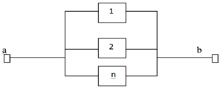
(b) Parallel structure:-

A system which is functioning which is called a parallel structure, if at least one of its n components is functioning the RBD is a parallel structure is shown below:-

Figure 5: - Reliability block diagram of a parallel structure

In this case we have connection between the end points a and b (i.e., the system is functioning) if we have connection through at least one of the blocks representing the components.

Reliability Block Diagrams versus Fault Trees:-

We have the alternative to choose whether to model the system structure by a fault tree or by a reliability block diagram when the fault tree is limited to only OR- gates and AND gates, both methods may yield the same result, and we may convert the fault tree to a reliability block diagram, and vice versa.

In a reliability block diagram, connection through a block means that the component represented by the block is functioning. Thus, again means that one or a specified set of a failure modes of the component is not occurring. In a fault tree we may let a basic event be the occurrence of the same failure mode or the same specified set of failure modes for the component.

We might start by constructing a fault tree instead of a reliability block diagram. In the construction of the fault tree we search for all potential causes of a specified system failure (accident). We think in terms of failures and will often reveal more potential failure causes than if we think in terms of functions, as, we do by establishing a reliability block diagram. The construction of a fault tree will give the analyst a better understanding of the potential causes of failure. If the analysis is carried out in the design phase the analyst may rethink the design and operation of the system and take actions to eliminate potential hazards.

[image:7.612.111.500.328.483.2]

(8)

International Journal of Emerging Technology and Advanced Engineering

It can be created by asking 'how' an established function is already accomplished.

This diagram may also be developed in the reverse direction by asking why a function is necessary. This is repeated until functions on the system level are reached.

Level of Indenture

Level 1 Functions

Level 2 Functions

[image:8.612.57.536.195.470.2]

Level 3 Functions

Figure 6: - Function tree

X. FUNCTIONAL ANALYSIS SYSTEM TECHNIQUE (FAST):- As a tool of functional analysis, society of American value Engineers in 1965 introduced FAST which is drawn from left to right, starting with the system function on the left side and ask 'how' this function is (or may be) accomplished.

The functions on the first level are then identified and entered into the diagram. We continue asking 'how' until we reach the intended level of detail. The lower level functions can be connected by AND and OR relations.

When OR

Why How

AND

When

Figure 7: - Symbols used in FAST Diagram

System Functions

Function

1.1 Function

1.2 Function

2.1 Function

2.2 Function

2.3 Function

1.1.2 Function

2.1.1 Function

2.1.2 Function

[image:8.612.58.520.564.721.2]

(9)

International Journal of Emerging Technology and Advanced Engineering

XI. STRUCTURED ANALYSIS AND DESIGN TECHNIQUE

(SADT)

This technique was developed by Douglas T. Ross of SofTech Inc. in 1973 as an approach to functional modeling. It has been widely used as a notation for system definition, process representation, software requirements analysis and software/system design. In the SADT diagram each functional block is modeled according to the same structure with following elements:- i) Function, ii) Input, iii) Control, iv) Mechanism, and v) Output.

SADT diagram can be very useful to model, the modules and the functions. For new system, SADT may be used to define the requirements and specify the functions and as a basis for suggesting a solution that meets the requirements and performs the functions. For existing systems SADT can be used to analyze the functions the system performs and to record mechanisms by which these functions are accomplished3.

XII. CAUSE IDENTIFICATION AND SELECTION OF BEST

PATH THROUGH PROPAGATION PROBABILITY NETWORK

FOR COMPONENT ASSEMBLAGE

So far we have discussed the components as an individual entity, its functional and structural analysis, assemblage of components as a system structure, now we discuss and propose a possible combination of components to make a system reliable as a whole.

Component- based software systems reliability is estimated using the reliability of the individual components and their interconnection mechanism. It is reasonable to think that an individual component is reliable, well tested, performs its intended functionality at individual level, but when interconnected with other components may behave unreliably. There might be certain components that do not perform correctly or their functions cannot be ascertained until after the composition. Such situations might undermine the reliability of the composed system.

Thus, the software systems composed of components may have a number of possible paths of interconnection and, therefore, execution. These paths can have a probability associated with them, what is called path propagation probability. It is, out of the number of possible paths, probability that a particular path of execution will be taken. In this, activation of certain components are considered for an individual path during an execution of overall system.

Reliability estimation through CAG:-

For estimating the reliability of a component based software system we can take into account the concept of propagation probability.

We can Construct Component Architecture Graph (CAG) based on various propagation probabilities. It is a directed graph. This architecture is expressed as a set of interacting components and the components are connected via a directed edge.

For reliability prediction to be more accurate and versatile we can divide the approach in two phases. First, we can do the failure diagnosis in the network graph of CBS. We can find the source node of error with the help of error propagation probability. Finding the source node of error, we can debug/ modify/ or replace the component with the new one and then perform testing to find whether there is an error. It is performed iteratively till there is no error in the network.

In the second phase, with the help of CAG and path propagation probability we can derive alternative testing paths, adjust transition probability and can evaluate each path reliability. It is done iteratively till the best approximation of path reliability is estimated.

For reliability estimation and right combination and connection (path) of components, propagation probabilities and node reliabilities can be attached along with component and transition edges. There can be so many alternative combinations of components but the combination which manifest perfectly and which is most reliable, would be the best selection. In a combination of components (CAG), in question, we attempt to check the final outcome, whether it is expected one. Hence in the first phase we attempt to find the erroneous component, that is, the root cause. If we are able to find the source component from where the error propagates to the component in question, we can attempt to remove the error or we might replace /deplete the erroneous source component. This we can do with the help of error propagation probability. For this we can construct network graph.

Network Graph:-

An error propagating network can be modelled as a directed graph.

G = (V, E).

Where V is the Vertices in the graph.

V = { V1, V2, ……….Vn }

which represents components in the network, and E is directed edges

E = { eij |ei is an edge from Vi to Vj }

Each edge eij has a propagation probability from Vi to

(10)

International Journal of Emerging Technology and Advanced Engineering

In case a node Vs fails, it starts propagating errors to its

neighbouring nodes. For each edge, error propagates with the associated propagation probability. This process of propagation is repeated for all remaining edges to propagate errors.

Monitors:-

In small network of components, identification of error source is not problematic because some of the nodes get infected with errors whereas other nodes are not infected with errors. This provides valuable information in identifying the error source.

But in case of large network of components, it is very time-consuming and difficult to check every node whether it is infected or not. Hence, in this case we can pre-select a set of nodes M which we can denote Monitors. These monitors report whether they are infected or not.

For a given error, M can be divided into two sets: Infected (M+) and uninfected monitors (M‾). The sets of infected monitors and uninfected monitors (M+,M‾) are called an outcome of an error. (Eun Soo, 2012). "Failure Diagnosis in Distributed Systems, Dissertation Submitted to University of Illinois). Given that a node 𝓋x is the error

source, outcome probability P (M+, M‾│𝓋x)) is the

probability that all infected monitors receive the error and no uninfected monitors receive the error.

Finding Error Source:-

Given a graph G (V, E), a propagation probability function and an outcome of error propagation (M+, M‾) from preselected monitors M, we attempt o find the node 𝓋x which maximizes P (M+, M‾ │ 𝓋x)

In the graph (tree) node 1 is the Source, we attempt to find node x is infected and node y is not infected by P(x+ y‾). The edge propagation probability can be denoted from node x to y by pxy.. For the node 4 to get infected (P (4

+

)) it should receive the error from node 2, so node 2 should be infected (P (2+ 4+)). Because node 1 is the source, nodes 1, 2 and 4 are infected ones (P (1+2+4+)). It does not matter whether node 3 is infected one or not. P (4+) is computed as P (4+) = P (2+ 4+)

= P (1+ 2+ 4+) = P12. P24

Given a source node 𝓋x and a monitor 𝓋m, there might

be a large number of paths from 𝓋x to 𝓋m , the exact end -to

end propagation probability becomes P(𝓋x𝓋m ) and it

becomes expensive. The approximate probability by taking a path that has the maximum propagation probability can be expressed as:-

𝓋x 𝓋m

ij

The path propagation probability (Π eij is in t pij) is

calculated by multiplying all edge propagation probabilities in the path.

This equation implies that errors are assumed to propagate through best paths in terms of the path propagation probability.

Since errors can actually propagate through non-best paths, P' (𝓋x 𝓋m) is only a lower bound of the exact error

propagation probability P' (𝓋x 𝓋m).

We can calculate the maximum path propagation probability as follows: For each edge eij, and edge weight

wij can be

wij log2 pij

As pij is in [0,1], wij is non- negative. The path with

maximum propagation probability from 𝓋x to 𝓋m is the

shortest path from 𝓋x to 𝓋m with respect to the newly

calculated edge weights wij.15

After we find the erroneous node, we start second phase to find the best alternative path, and finally the overall system reliability. To perform this, certain assumptions are required to be made. We have to assume that individual component reliability is known. All components are physically independent of each other. The bug fixing does not introduce new errors. The next component to be executed depends only on the current component. We take into consideration only those components which get activated during execution. We do not consider those components which do not get activated during execution. Component usage ratio is also computed, which is the ratio of a particular component execution time over the total software system execution time9. The value of component usage ratio is 0 i The addition of usage ratio of all

components is equal to 1

1

2

3

(11)

International Journal of Emerging Technology and Advanced Engineering

∑ i

This ratio can be calculated if the values of total component execution time (T(Ci)) and total software

execution time (T(S)) are known for a component i. The possible approach for calculating usage ratio of a component is

i

This equation describes that the usage ratio of component i is equal to the total ith component execution time (T(Ci)) over the total system execution time (T(S)).

The usage time ratio is a fixed quantity and does not change with varying inputs or sets of operations executed12. The component usage ratio weights the impact of component reliabilities on the software system reliability.

The impact factor Ik for component k is evaluated as:-

Ik = ∑

As a general rule the component which is frequently executed has more impact on the system reliability than the component which is rarely executed10,11. Also, the component which consumes much of the total execution time have more impact on the overall reliability of the system than that of the components that consumes less execution time.

After the computation of component usage ratio for individual component, Path Propagation Probability is derived12. The path Propagation Reliability depends on the decisions taken at component level which then decide the due course of the path13.

Now reliability RCBS for whole component based

software is estimated with node reliabilities Ri, and

transition probability Pij (ΣiΣj Pij = 1).

RCBS =

∑ i j

where m is number of available transitions for selected testing path. The overall reliability of CBS is a function including summation of terms weighted by transition probability, where each term is a summation of individual component reliabilities of a selected execution path14.

Therefore computation of overall system reliability is made by computation of reliability of individual component. If R (Ci) is the reliability of ith component of the system and R(S) is the overall system reliability, then

R(S) = ψ { R (C1), R(C2), …………..R(Cn)}

Let the total time period of the execution of the software is T(s), N is total no. of times the process input data in its life time is fi times the component i participated in the

execution process if the average time taken by component i is ti for T(Ci) = ti × fi different set of inputs then the total

usage time of component i is 1

T(s) = t1 ×f1 + t2 ×f2 + t3 ×f3 +………. tn ×fn

where n is the total no. of components in software system

Usage ratio =

f1+f2 +…………..+fn = N

=

Let P1, P2, P3, ……….., Pk are identified paths for total no. of available paths-k paths -K for all sorts of inputs . Probability of path selection - p1, p2, p3, ……..Pk is random

∑

Let the probability of failure of component Cj is fi, j ,

where Cj ⋲ Pj Then the probability of non failure is (1-fi, j)

Hence the probability that the path will survive will be

∏ ( )

Let N is the total no. of processes processed by the software and n1, n2, ………..nk are the frequency of the

path P1, P2, P3, ……….Pk then,

n1 +n2+ ……….+nk= N

Where n1 = p1.N, n2 = p2.N, …………nk = pk .N ∴ R(s) Ψ { R(C1), R(C2), ……….. , R(Cn)}

and R(Pi) ζ { R(Ci), where Ci ⋲ Pi }

∴R(S) φ { R(P1), R(P2), ………..R(Pk) }

Then the reliability of the system R(S) can be the weighted mean of RP1, RP2, ……….., RPk.

Hence, R(S) =

or R(S)= p1 × RP1+ p2× RP2+………….+pk× RPk

(12)

International Journal of Emerging Technology and Advanced Engineering

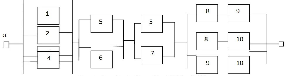
Website: www.ijetae.com (ISSN 2250-2459, ISO 9001:2008 Certified Journal, Volume 7, Issue 9, September 2017) For numerical simulation we consider the following graph:-

In this figure there is one entry point - C1 and one exit

point - C9. Thus, the possible paths in this figure are:-

P1 (C2 C3 C4 C6 C9 )

P2 (C2 C3 C5 C6 C9 )

P3 (C2 C9)

P4 (C2 C7 C8 C9 )

If the failure probability of all the components are supposed to be 0.02, then

R (Pj) = ∏ ( )

R (P j) = ∏

∏

=

Following the figure

R (P1) = (0.98)5 = 0.9039

R (P2) = (0.98)5 = 0.9039

R (P3) = (0.98)2 = 0.9604

R (P4) = (0.98) 4

= 0.9223

∴ +

Assuming corresponding probabilities for p1, p2, p3 and p4

by for each path, P1, P2, P3, and P4, as 0.3, 0.2, 0.4, and 0.1

we have

R(s) = 0.3 0.9039+ 0.2 0.9039+04. 0.9604+0.1 0.9223

R(s) = 0.92834

Therefore, system reliability seems to be 92.83%.

Algorithm15:-

Phase 1: Find Erroneous node by constructing network graph (CAG): G = (V, E)

Case1: Small network of components

Find a node Vs that fails

For each edge find error propagation with the associated propagation probability

Find neighboring nodes where error is propagated by node Vs

Repeat the process of propagation until there is

remaining edge to propagate

Find the Source node of error

Case 2: Large network of components

C

3

C

7

C

1

C

2

C

4

C

8

C

6

C

9

(13)

International Journal of Emerging Technology and Advanced Engineering

Input T: Shortest path tree from 𝓋s to all

monitors.

Input 𝓋s : Root of error propagation

Pre-select a set of nodes as Monitor

Input M + and M : Positive/ uninfected monitors. For a given error divide M into two sets

a. Infected Errors

M

+

b. Uninfected Errors M

Outcome of an error is (M+, M ) – sets of infected and uninfected Monitors.

P (M+, M │Vx) for a given source node Vx is the

probability that all infected monitors receive error

and no uninfected errors receive the error.

Select node1 as the source,

attempt to find infected node x and uninfected node y by P(X+ y ).

Px,y denotes edge propagation probability from node x

to node y.

P( ) gives exact end–to–end propagation

probability for a large no. of paths from a given

source node and a monitor

Phase ii: Finding the best alternative path and overall system reliability.

Assume reliability of individual component is known. Assume all components are physically independent of each other

Bug fixing does not introduce new errors.

Next component to be executed depends only on the current component.

Consider only those components that get activated during execution.

Leave those components that remain inactive during execution.

Compute component usage ratio (φi) which is 0< φi <1

- Find total component execution time (T(Ci))

- Find total software execution time T(s))

- Find component usage ratio as

φi =

Compute Impact Factor of Component Ik for component

k as

∑

Derive path propagation probability to identify the probable path of execution out of no. of possible paths.

- Decide a testing path and test each component - Adjust transition probability

- Evaluate path reliability

- Iteratively perform testing and evaluating each path by changing parameters

Estimate software reliability with estimates of path reliabilities.

Estimate reliability RCBS for selected execution path

with node reliabilities Ri andtransition probability Pij (Σi Σj

Pij = 1)

RCBS =

∑

for m- the no. of available

transition for selected testing path.

REFERENCES

[1] Clements, P., "From Subroutines to Subsystem: Component Based Software Development," American Programmer, vol. 8, no. 11, Nov. 1995.

[2] Yourdon. E, " Software Reuse", Application Development Strategies, vol. VI, no. 12, December 1994, pp. 1-16.

[3] Pour. G, "Software Component Technologies: JavaBeans and ActiveX”, Proceedings of Technology of Object-Oriented language and Systems, 1999, pp. 398-398.

[4] MIL-STD-882D. 2000. Standard Practice for System Safety. U.S. Department of Defense, Washington, DC.

[5] IEC 50 (191). 1990. International Electrotechnical Vocabulary (IEV) - Chapter 191- Dependability and Quality of Service. International Electrotechnical Commision, Geneva.

[6] IEEE Std. 352. 1982. IEEE Guide for General Principles of Reliability Analysis of Nuclear Power Generating Station Protection Systems. IEEE New York.

[7] Lissandre, M. 1990. Maitriser SADT Albert Colin, Paris.

[8] Douglas T. Ross, of SofTech Inc. in 1973, SADT "Structural Anlysis and Design technique ",

[9] Cheung, R. C., 1980" "A User Oriented Software Reliability Model, IEEE Transactions on Software Engineering, SE - 6(2), 118-125). [10] Goel, A. L., K. Okumoto, 1979: " A Time -dependent Error

(14)

International Journal of Emerging Technology and Advanced Engineering

[11] Gokhale, S.S. &K.S. Trivedi, 2006: "Analytical Models for Architecture -Based Software Reliability Prediction: A Unication Framework, IEEE Trans. on Rel., 55(4), 578-590.)

[12] Goswamy, Vivek and Y.B. Acharya 2009: "Method of Reliability Estimation of COTS Components based Software Systems", Proceedings of 20th_{International Symposium on Software Reliability}

Engineering, ISSRE.

[13] Nautiyal, L., Neena Gupta, Sushil Chandra Demri (2013): "A new path based reliability approach for estimation of reliability of Component Based Software Development", Int. Jour. of Comp. Sc. Engg., Vol. 2, No. 06, 2013.

[14] Singh, A.P. and P. Tomar, "A proposed methodology for reliability estimation of component- based software, Int. Conf. on Optimization Modeling and Applications, 2012.