Optimization of Cutting Parameters in Ti alloy during CNC Turning

(1)

International Journal of Emerging Technology and Advanced Engineering

Website: www.ijetae.com (ISSN 2250-2459, ISO 9001:2008 Certified Journal, Volume 7, Issue 9, September 2017)

311 Optimization of Cutting Parameters in Ti alloy during CNC

Turning

Sachin Sharma

1

, Akash Singh

2

, Shubham Sharma

3

, Umesh Kumar Vates

4

, Gyanendra Kumar Singh

5

1,2

B.Tech student at Department of Mechanical Engineering, Amity University Uttar Pradesh, Noida 2,3, 4, 5_{Faculties at Department of Mechanical Engineering, Amity University Uttar Pradesh, Noida}

Absract-- Present work aimed to improve the quality and minimize the cost during turning operation of Ti-6Al-4V alloy. The optimum cost and quality can be achieved by the selection of optimum machining parameters. Series of experiments were conducted to find the effect of machining parameters during turning operation. The main parameters taken for the study are feed rate, cutting speed(spindle speed),concentration of coolant and depth of cut and their effect is observed on the surface finish and material removal rate (MRR) of Ti-6Al-4V Alloy. A mathematical tool called Design of experiment was developed in terms of output parameters (surface roughness and MRR). The effect of machining parameters on the surface texture and material removal rate has been investigated by using three factor box behnken Response Surface Method (RSM). 3D plots were constructed to find the optimum parameters required for better surface finish and higher material removal rate. The conclusion is drawn that the feed rate is the main machining parameter that affects the surface roughness. A small change in feed results in major change on surface roughness. The surface irregularities were found to be directly proportional to feed as increase in the feed rate results in increase in surface irregularities.

Keyword: Ti-6Al-4V alloy, RSM, MRR, SR.

I. INTRODUCTION

With the advancement of technology and modern manufacturing techniques, the machining parameters are required to be more precise. Surface finish is one of the major factor considered as the scale of product quality. As a product’s life and functionality is considered as directly proportional to the surface finish. Surface quality influences the performance of the product by affecting factors includes friction during rubbing, simplicity of holding product, conductivities, and many more. With the quality, attention is also paid to the product’s cost while manufacturing. As with the quality the product should be economical too and the cost during turning operation can be reduced by improving the material removal rate which in turns reduces the machining time. Higher the material removal rate minimum is the machining time and lesser is the cost. The factors that affects surface texture are cutting parameters as speed and feed ,tool structure, mechanical and chemical properties of work piece and cutting conditions including conc. of coolant, temperature etc .

As observed, in turning the surface roughness and MRR depends on parameters as spindle speed, feed rate, depth of cut, tool nose radius, and lubrication of the cutting tool, machine vibrations, tool wear and on other mechanical properties of the material. Any change in machining parameters results in significant change on the produced surface texture.

This makes important for the researchers and scholars to find the optimum machining parameters and to establish the relationship between these affecting parameters. Material removal rate influences the machining time which in turns affects the production cost of the material. The determination of this relationship between these parameters is always remains as an open field for research, mainly because of the advancements in modern technologies in machining process. In machining investigations, design of experiment is used to perform the experiment. Design of experiment is the process of planning the experiments, fixing the different values of the different parameters so that the appropriate data can be obtained and analyzed, resulting in valid conclusions [2].For the performing experiment, there are several ways provided to draft the design of experiment (DOE). There are several modern technologies to draft DOE such as factorial designs, response surface methodology (RSM) and taguchi method. And the traditional approach includes one factor at a time experimental. The modern techniques are preferred over traditional approach because of its less time consuming and cost.

(2)

International Journal of Emerging Technology and Advanced Engineering

312

Previous studies done in the field of turning operation shows the efforts to find the effect of cutting conditions like spindle speed, depth of cut and feed on surface roughness as well as with less number of trials.

Present study deals with the effect of cutting speed(spindle speed), feed ,depth of cut and concentration of coolant on the surface roughness and material removal rate by 27 number of experiments.

Noordin et al. [7] sketch the design of experiment using response surface methodology. The tool material used is of coated carbide for the turning of AISI 1045 steel. The conclusion is set that feed was the most important parameter that influences the surface texture.

Choudhury and El-Baradie [10] concluded that cutting speed was the main affecting parameter on the tool damage.

Suresh et al. [8] have drafted the experiment using RS methodology. They used mild steel to find the factor affecting the process parameters.

Paulo Davim [13] used the taguchi methodology to sketch the DOE and concluded that cutting speed influences most on the roughness followed by the feed. It is also concluded that depth of cut has no major influence on roughness.

Mohamed Dabnum et al. [22] performed the experiment on glass ceramic (MACOR). The DOE was made using response surface methodology. The conclusion given by them is that the feed rate was the major influencing factor on the roughness, followed by cutting speed.

Munoz and Cassier [11] predicted the model for surface roughness. They used different types of steel such as AISI 1020, AISI 1045 and AISI 4140. They concluded that surface irregularities decreases by increasing cutting speed and tool nose radius and by increasing the feed rate. The depth of cut does not majorly affect the surface roughness.

Thiele and Melkote [3] constructed the DOE with three-factor complete three-factorial design. They worked on to determine the influence of work piece hardness and tool geometry on surface texture and machining forces. They predicted that the affect of interaction of the edge geometry and hardness of work piece on the surface roughness is also important.

Nikolaos et al. [19] used the DOE with 23 full factorial design. They predicted that for AISI 316L steel variables named feed, speed and depth of cut influence the most. The relation proved that the depth of cut was the major influencing parameter for the surface finish. It improves with decreasing the depth of cut and feed rate respectively, but it decreased with increasing the cutting speed.

Nikos [20] used RSM and fuzzy logic system for Ti6Al4 V alloy. The feed was found as the major influencing factor for the surface finish.

Lalwani et al. [21] used Response Surface Methodology for examining the machining factor affecting on cutting forces and roughness in turning of MDN250 steel and concluded that better surface finish can be obtain when speed and depth of cut are set to their high level of the experimental range and feed is set at low level.

Choudhury and EL-Baradie [23] sketched a model using response surface methodology. They used EN 24T for turning and checks the influence on surface roughness. They predicted that the influence of feed rate is more than the affect of speed and depth of cut. However, a higher cutting speed improves the surface texture.

Mital and Mehta [4] developed model for factors

affecting the surface roughness. They performed

experiment on aluminum alloy 390, ductile cast iron, medium carbon leaded steel, medium carbon alloy steel 4130, and inconel 718 and predicted that cutting speed, feed rate and tool nose radius have major impact on surface texture.

Fang and Wang [12] drafted the DOE for surface roughness using two level fractional factorial. They considered machining parameters as hardness of work piece, feed, tool angles and speed Sundram and Lambert

[5,6] sketch the model for surface roughness. The work piece used is of AISI 4140 steel during the turning operation.

In this study effort has been made to develop the surface roughness and material removal rate prediction model of Ti-6AI-4V titanium alloy with the use of modern method under variable cutting conditions. By using response surface methodology and (27)box benken full factorial design of experiment, quadratic model has been developed.

II. EXPERIMENTAL WORK

(3)

International Journal of Emerging Technology and Advanced Engineering

313

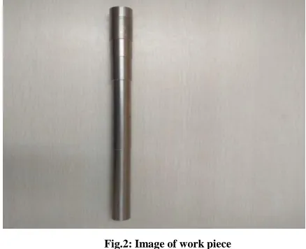
[image:3.612.317.572.249.721.2]

All of the 27 experiments were conducted on CNC Lathe of Jobber XL model made by Ace design. The specifications of the CNC lathe machine are spindle speed that can vary between a range of 100–1500 RPM and having motor of 7.5 KW power. Surface roughness is measured by inspecting the finer irregularities of the surface texture and this is done by a digital surface test device of model No. SJ-400 by Mitutoyo. For measuring the material removal rate work piece is removed from the lathe after each experiment and weighed on machine made by metic. The time for each experiment is kept fixed i.e. 1 minute. The MRR for each experiment is found by reduction of the mass during machining. The surface roughness was measured at five different points around the circumference of the work pieces to obtain more accurate value and finally the mean of five values is taken for the calculations. In the experiment, the work piece was the Ti-6Al-4V alloy rod of 1 inch diameter. This material has high tensile stress, tough and is corrosion resistance, used for the manufacturing different military product and components in which high tensile stress is most important factor.

Fig.2: Image of work piece

Input machining parameters and their levels.

S.No. Input Parameters Level 1 Level 2 Level 3 1 Cutting speed (v)

m/min

200 400 600

2 Feed (f) mm/rev 0.05 0.1 0.15 3 Depth of cut (d) mm 0.2 0.4 0.6 4 Concentration of

coolant (c)

[image:3.612.48.267.387.565.2]

20 25 30

Table 2

Mechanical properties of Ti-6Al-4V alloy.

Properties Values

Hardness (HRC) 36 Ultimate tensile strength 950 MPa Poisson’s ratio 0.342 Modulus of elasticity 113 GPa

Density 4.43 g/m3

Thermal conductivity 6.7W/mK

Table 3:

Chemical composition of Ti-6Al-4V alloy.

Element Percentage

Ti 89.55

Al 6.40

V 3.89

Fe 0.16

C 0.002

Table: 4- Experimental Observations

SL Conc .

Depth of Cut (mm)

Feed (mm)

Cutting Speed

MRR (g/mm)

SR (nm) 1 30 0.2 0.10 400 2.2 590 2 20 0.4 0.15 400 1.9 764s

3 20 0.2 0.1 400 0.6 678

4 30 0.4 0.15 400 6.6 575

5 25 0.6 0.1 600 10.3 630

6 25 0.4 0.15 200 5 428

7 20 0.4 0.1 200 1 360

8 20 0.4 0.05 400 1.9 466

9 30 0.4 0.05 400 2.2 543

10 20 0.6 0.1 400 10 390

11 30 0.6 0.1 400 6 350

12 25 0.6 0.15 400 9.2 728

13 25 0.6 0.05 400 3.1 353

14 30 0.4 0.1 600 7.3 610

15 25 0.2 0.1 600 3.4 345

16 25 0.4 0.05 200 1.3 368

17 25 0.2 0.05 400 1.6 265

18 25 0.4 0.05 600 3.8 440

19 25 0.4 0.15 600 11 525

20 20 0.4 0.1 600 1.6 424

21 25 0.2 0.15 400 4.1 428

22 25 0.4 0.1 400 5.3 425

23 30 0.4 0.1 200 2.2 543

24 25 0.4 0.1 400 5.3 458

25 25 0.4 0.1 400 5.3 413

26 25 0.2 0.1 200 1.2 370

[image:3.612.45.291.587.670.2]

(4)

International Journal of Emerging Technology and Advanced Engineering

314

III. RESULT

Residual plot for surface roughness (Ra)

Fig.3: Residual Plot for SR

The normal probability curve for surface roughness (Ra) validates the experimental data obtained while machining the titanium alloy on CNC. The linear line is the expected values and the dots are the observed values and the dot along the line shows that the experiment is good. The versus fit drawn around the 0 line and the randomness is observed in the graph which also validate the experiment. It is valid because of randomness. The histogram is the transformation of versus graph using any operation (mainly logarithmic), The versus order is graph drawn by connecting the observed values around a initial line of 0.

Residual plot for MRR

Fig.4: Residual Plot for MRR

The normal probability curve for Material removal rate (MRR) validates the experimental data obtained while machining the titanium alloy on CNC. The linear line is the expected values and the dots are the observed values and the dots along the line shows that the experiment is good. There is one outlier (extremely unexcpected) value is found.

The versus fit drawn around the 0 line and the randomness is observed in the graph which also validate the experiments. It is valid because of randomness. The histogram is the transformation of versus graph using any operation (mainly logarithmic), The versus order is graph drawn by connecting the observed values around a initial line of 0.

200 100 0 -100 -200 99 90 50 10 1 Residual P e r c e n t 700 600 500 400 300 200 100 0 -100 -200 Fitted Value R e s id u a l 200 100 0 -100 -200 8 6 4 2 0 Residual F r e q u e n c y 26 24 22 20 18 16 14 12 10 8 6 4 2 200 100 0 -100 -200 Observation Order R e s id u a l

Normal Probability Plot Versus Fits

Histogram Versus Order

Residual Plots for Ra

3.0 1.5 0.0 -1.5 -3.0 99 90 50 10 1 Residual P e r c e n t 10.0 7.5 5.0 2.5 0.0 2 0 -2 Fitted Value R e s id u a l 3 2 1 0 -1 -2 10.0 7.5 5.0 2.5 0.0 Residual F r e q u e n c y 26 24 22 20 18 16 14 12 10 8 6 4 2 2 0 -2 Observation Order R e s id u a l

Normal Probability Plot Versus Fits

Histogram Versus Order

(5)

International Journal of Emerging Technology and Advanced Engineering

315

Surface plot for MRR vs speed and feed.

Fig.5: Scattered Plot for MRR1

The surface plot of MRR vs. speed, feed shows that when the concentration and depth of cut is held constant at values (observation-6,16,18,19,22,25and 26)it is observed that with increase in feed and speed the MRR increases for lower values of feed and speed. the MRR observed is also low and when feed and speed is increased MRR increases with them .

So we can say that for mid values of depth of cut and concentration the MRR is directly proportional to feed and speed.

Surface plot for MRR vs speed , depth of cut

The surface plot of MRR vs speed and depth of cut shows that when the concentration and feed is held constant at values (observation-5,15,22,24,25,26 and 27 )it is observed that with increase in speed and depth of cut the MRR increases for lower values of depth of cut and speed. The MRR increase with increases in speed and depth of cut. So we can say that for mid values of feed and concentration the MRR is directly proportional to depth of cut and speed.

Surface plot of MRR vs feed, depth of cut

The surface plot of MRR vs depth of cut and feed shows that when the concentration and depth of cut is held constant at values (observation-6, 16,18,19,22,25and 26)it is observed that with increase in feed and speed the MRR increases for lower values of feed and speed. The MRR observed is also low and when feed and speed is increased MRR increases with them. So we can say that for mid values of depth of cut and concentration the MRR is directly proportional to feed and speed.Contour plot of MRR vs speed, feed

2 4 6

0.05 0.05

0.10 0.05 8

400 200 0.15

600

MRR

speed

feed

Concentration 25 Depth of cut 0.4 Hold Values

Surface Plot of MRR vs speed, feed

3 6

0.2 0.2

0.4 0.2 9

200 0.6

400 600

MRR

speed

Depth of cut

Concentration 25 feed 0.1 Hold Values

Surface Plot of MRR vs speed, Depth of cut

3 6

0.2 0.4 0.2

0.4 9

0.05 0.6

0.10 0.15

MRR

feed

Depth of cut

(6)

International Journal of Emerging Technology and Advanced Engineering

316

Fig.8: Contour Plot for MRR1

When the concentration and depth of cut are held constant and the effect of speed and feed is observed on MRR it is seen that low MRR is found in region where speed as well as feed is low and high MRR is found when feed as well as speed are very high.

Contour plot of MRR vs speed, depth of cut

When the concentration and feed are held constant and the effect of speed and depth of cut is observed on MRR it is seen that low MRR is found in region where speed as well as depth of cut is low and high MRR is found when depth of cut as well as speed are very high.

Contour plot of MRR vs feed, depth of cut

When the concentration and speed are geld constant and the effect of feed and depth of cut is observed on MRR it is seen that low MRR is found in region where feed as well as depth of cut is low and high MRR is found when depth of cut as well as fee are very high.

Contour plot of MRR vs speed, concentration

When the depth of cut and feed is held constant at their mid values and effect of speed and concentration on MRR is observed it is seen that low MRR is obtained only when speed is very low and concentration very high. High MRR is obtained when speed is high as well as the concentration. Contour plot of MRR vs feed, concentration.

feed s p e e d 0.150 0.125 0.100 0.075 0.050 600 500 400 300 200 Concentration 25 Depth of cut 0.4 Hold Values

> – – – < 2

2 4

4 6

6 8

8 MRR

Contour Plot of MRR vs speed, feed

Depth of cut

sp ee d 0.6 0.5 0.4 0.3 0.2 600 500 400 300 200

C oncentration 25

feed 0.1 Hold Values > – – – – < 2

2 4 4 6 6 8 8 10 10 MRR

Contour Plot of MRR vs speed, Depth of cut

Depth of cut

fe ed 0.6 0.5 0.4 0.3 0.2 0.150 0.125 0.100 0.075 0.050 Concentration 25 speed 400 Hold Values > – – – – < 2 2 4 4 6 6 8 8 10 10 MRR

Contour Plot of MRR vs feed, Depth of cut

Concentration sp ee d 30 28 26 24 22 20 600 500 400 300 200

Depth of cut 0.4

feed 0.1 Hold Values > – – – – – < 2

2 3 3 4 4 5 5 6 6 7 7 MRR

(7)

International Journal of Emerging Technology and Advanced Engineering

317

When the depth of cut and speed is held constant at their mid values and the effect of concentration and feed is observed on MRR it is observed that lowest MRR is found in two cases when feed is very low and either concentrations is very low or very high. High MRR is found in the region when feed is very high and so as the concentration.

Contour plot of MRR vs depth of cut, concentartion

When feed and speed are held constant at their mid values and the effect of depth of cut and concentration is checked on MRR then it is concluded that when the depth of cut and concentration is less then MRR is also very less , high MRR is found when the depth of cut is very high and the concentration of coolant is medium . But major MRR is found in two regions when the depth of cut as well as the concentration is medium.

Optimization plot

Fig.14: Optimization Plot for MRR and SR

The optimal values of MRR and surface roughness is found to be 8.3570 and 449.6915 when the values of different input factors namely concentration, depth of cut feed and speed is taken 24.1414,0.60,0.09504 and 482.8283 respectively when there were no extra conditions for optimality were put on them, The total desirability of the of the experiment were .8911 that means if the surface roughness and mrr are to be collectively considered as desired output then it is only 89.11 percent efficient and found only on certain (in this case optimal) values of inputs.

Response Surface Regression: MRR versus Concentration, Depth of cut, feed, speed Estimated Regression Coefficients for MRR

Term Coef SE Coef T P Constant 5.30000 0.9358 5.664 0.000 Concentration 0.79167 0.4679 1.692 0.116 Depth of cut 2.44167 0.4679 5.218 0.000 feed 1.99167 0.4679 4.257 0.001 speed 1.90833 0.4679 4.079 0.002 Concentration*Concentration -1.43333 0.7018 -2.042 0.064 Depth of cut*Depth of cut 0.06667 0.7018 0.095 0.926

Concentration

fe

ed

30 28 26 24 22 20 0.150

0.125

0.100

0.075

0.050

Depth of cut 0.4 speed 400 Hold Values

> – – – – – < 2 2 3 3 4 4 5 5 6 6 7 7 MRR

Contour Plot of MRR vs feed, Concentration

Concentration

D

e

p

th

o

f

cu

t

30 28 26 24 22 20 0.6

0.5

0.4

0.3

0.2

feed 0.1 speed 400 Hold Values > – – – – – < 0.0 0.0 1.5 1.5 3.0 3.0 4.5 4.5 6.0 6.0 7.5 7.5 MRR

Contour Plot of MRR vs Depth of cut, Concentration

Cur

High Low 0.89111D Optimal

d = 0.91962 MaximumMRR

y = 8.3570

d = 0.86348 MinimumRa

y = 449.6915

0.89111 DesirabilityComposite

200.0 600.0 0.050

0.150 0.20

0.60 20.0

30.0 Depth of feed speed

Concentr

(8)

International Journal of Emerging Technology and Advanced Engineering

318

feed*feed -0.40833 0.7018 -0.582 0.571 speed*speed -0.38333 0.7018 -0.546 0.595 Concentration*Depth of cut -1.40000 0.8104 -1.728 0.110 Concentration*feed 1.10000 0.8104 1.357 0.200 Concentration*speed 1.12500 0.8104 1.388 0.190 Depth of cut*feed 0.90000 0.8104 1.111 0.289 Depth of cut*speed 1.07500 0.8104 1.326 0.209 feed*speed 0.87500 0.8104 1.080 0.302

S = 1.62083 PRESS = 181.584

R-Sq = 87.04% R-Sq(pred) = 25.37% R-Sq(adj) = 71.93%

Analysis of Variance for MRR

Source DF Seq SS Adj SS Adj MS F P Regression 14 211.800 211.800 15.1286 5.76 0.002 Linear 4 170.363 170.363 42.5908 16.21 0.000 Concentration 1 7.521 7.521 7.5208 2.86 0.116 Depth of cut 1 71.541 71.541 71.5408 27.23 0.000 feed 1 47.601 47.601 47.6008 18.12 0.001 speed 1 43.701 43.701 43.7008 16.63 0.002 Square 4 12.769 12.769 3.1923 1.22 0.355 Concentration*Concentration 1 11.065 10.957 10.9570 4.17 0.064 Depth of cut*Depth of cut 1 0.448 0.024 0.0237 0.01 0.926 feed*feed 1 0.472 0.889 0.8893 0.34 0.571 speed*speed 1 0.784 0.784 0.7837 0.30 0.595 Interaction 6 28.668 28.668 4.7779 1.82 0.178 Concentration*Depth of cut 1 7.840 7.840 7.8400 2.98 0.110 Concentration*feed 1 4.840 4.840 4.8400 1.84 0.200 Concentration*speed 1 5.062 5.062 5.0625 1.93 0.190 Depth of cut*feed 1 3.240 3.240 3.2400 1.23 0.289 Depth of cut*speed 1 4.623 4.623 4.6225 1.76 0.209 feed*speed 1 3.063 3.063 3.0625 1.17 0.302 Residual Error 12 31.525 31.525 2.6271

Lack-of-Fit 10 31.525 31.525 3.1525 * * Pure Error 2 0.000 0.000 0.0000

Total 26 243.325

Unusual Observations for MRR

Obs StdOrder MRR Fit SE Fit Residual St Resid 10 10 10.000 6.983 1.238 3.017 2.88 R

R denotes an observation with a large standardized residual.

Estimated Regression Coefficients for MRR using data in uncoded units

(9)

International Journal of Emerging Technology and Advanced Engineering

319

Depth of cut*speed 0.0268750

feed*speed 0.0875000

Response Surface Regression: Ra versus Concentration, Depth of cut, feed, speed The analysis was done using coded units.

Estimated Regression Coefficients for Ra

Term Coef SE Coef T P Constant 432.000 73.82 5.852 0.000 Concentration 10.750 36.91 0.291 0.776 Depth of cut 11.917 36.91 0.323 0.752 feed 84.417 36.91 2.287 0.041 speed 44.750 36.91 1.212 0.249 Concentration*Concentration 89.750 55.37 1.621 0.131 Depth of cut*Depth of cut -10.000 55.37 -0.181 0.860 feed*feed 38.500 55.37 0.695 0.500 speed*speed -20.500 55.37 -0.370 0.718 Concentration*Depth of cut 12.000 63.93 0.188 0.854 Concentration*feed -66.500 63.93 -1.040 0.319 Concentration*speed 0.750 63.93 0.012 0.991 Depth of cut*feed 53.000 63.93 0.829 0.423 Depth of cut*speed 71.750 63.93 1.122 0.284 feed*speed 6.250 63.93 0.098 0.924

S = 127.863 PRESS = 1126236

R-Sq = 54.03% R-Sq(pred) = 0.00% R-Sq(adj) = 0.40%

Analysis of Variance for Ra

Source DF Seq SS Adj SS Adj MS F P Regression 14 230608 230608 16472.0 1.01 0.500 Linear 4 112636 112636 28158.9 1.72 0.210 Concentration 1 1387 1387 1386.8 0.08 0.776 Depth of cut 1 1704 1704 1704.1 0.10 0.752 feed 1 85514 85514 85514.1 5.23 0.041 speed 1 24031 24031 24030.7 1.47 0.249 Square 4 67720 67720 16930.1 1.04 0.429 Concentration*Concentration 1 51803 42960 42960.3 2.63 0.131 Depth of cut*Depth of cut 1 1346 533 533.3 0.03 0.860 feed*feed 1 12331 7905 7905.3 0.48 0.500 speed*speed 1 2241 2241 2241.3 0.14 0.718 Interaction 6 50252 50252 8375.3 0.51 0.788 Concentration*Depth of cut 1 576 576 576.0 0.04 0.854 Concentration*feed 1 17689 17689 17689.0 1.08 0.319 Concentration*speed 1 2 2 2.3 0.00 0.991 Depth of cut*feed 1 11236 11236 11236.0 0.69 0.423 Depth of cut*speed 1 20592 20592 20592.3 1.26 0.284 feed*speed 1 156 156 156.3 0.01 0.924 Residual Error 12 196189 196189 16349.1

Lack-of-Fit 10 195103 195103 19510.3 35.93 0.027 Pure Error 2 1086 1086 543.0

Total 26 426797

Unusual Observations for Ra

(10)

International Journal of Emerging Technology and Advanced Engineering

320

R denotes an observation with a large standardized residual.

Estimated Regression Coefficients for Ra using data in uncoded units

Term Coef Constant 2358.33 Concentration -155.850 Depth of cut -1287.92 feed 2888.33 speed -0.165000 Concentration*Concentration 3.59000 Depth of cut*Depth of cut -250.000 feed*feed 15400.0 speed*speed -5.12500E-04 Concentration*Depth of cut 12.0000 Concentration*feed -266.000 Concentration*speed 0.000750000 Depth of cut*feed 5300.00 Depth of cut*speed 1.79375 feed*speed 0.625000

Response Optimization Parameters

Goal Lower Target Upper Weight Import MRR Maximum 2 10 10 1 1 Ra Minimum 350 350 700 1 1

Global Solution

Concentratio = 24.0404 Depth of cut = 0.6 feed = 0.0893939 speed = 462.626

Predicted Responses

MRR = 8.056 , desirability = 0.757022 Ra = 436.742 , desirability = 0.752166

Composite Desirability = 0.754590

Optimization Plot Response Optimization

Parameters

Goal Lower Target Upper Weight Import MRR Maximum 1 9 9 1 1 Ra Minimum 400 400 764 1 1 Global Solution

Concentratio = 24.1414 Depth of cut = 0.6 feed = 0.0904040 speed = 482.828 Predicted Responses

(11)

International Journal of Emerging Technology and Advanced Engineering

321

Response Optimization

Parameters

Goal Lower Target Upper Weight Import MRR Maximum 1 9 9 1 1 Ra Minimum 400 400 764 1 1

Global Solution

Concentratio = 24.1414 Depth of cut = 0.6 feed = 0.0904040 speed = 482.828 Predicted Responses

MRR = 8.357 , desirability = 0.919625 Ra = 449.692 , desirability = 0.863485 Composite Desirability = 0.891113

IV. CONCLUSION

In this study, application of RSM (unblocked box behiken) on the Tu-6AI-4V is carried out for turning operation. A quadratic model has been developed for surface roughness (Ra) and material removal rate to

investigate the influence of machining parameters. The results are as follow:

1.For the surface roughness, the feed rate is the main influencing parameter on the roughness, followed by the cutting speed. A depth of cut does no influences the surface roughness.

2.It can be seen that interaction between most parameters has no significant influence except feed rate.

3.3D surface counter plots are used to determine the optimum condition for particular values of surface finish.

4.Verification experiments performed show that the empirical models developed can be used for turning of Ti-6Al-4V alloy within 6% error.

REFERENCES

[1] G. Boothroyd, W.A. Knight, Fundamentals of Machining and Machine Tools, third ed., CRC press, Taylor & Francis Group, 2006. [2] D.C. Montgomery, Design and Analysis of Experiments, fourth ed.,

John Wiley & sons Inc., 1997.

[3] J.D. Thiele, S.N. Melkote, Effect of cutting edge geometry and work piece hardness on surface generation in the finish hard turning of AISI 52100 steel, J. Mater. Process. Technol. 94 (1999) 216–226. [4] A. Mittal, M. Mehta, Surface finish prediction models for fine

turning, Int. J. Prod. Res. 26 (12) (1988) 1861–1876.

[5] R.M. Sundaram, B.K. Lambert, Mathematical models to predict surface finish in fine turning of steel, Part 1, Int. J. Prod. Res. 19 (5) (1981) 547–556.

[6] R.M. Sundaram, B.K. Lambert, Mathematical models to predict surface finish in fine turning of steel, Part 2, Int. J. Prod. Res. 19 (5) (1981) 557–564.

[7] M.Y. Noordin, V.C. Venkatesh, S. Sharif, S. Elting, A. Abdullah, Application of response surface methodology in describing the performance of coated carbide tools when turning AISI 1045 steel, J. Mater. Process. Technol. 145 (2004) 46–58.

[8] P.V.S. Suresh, P.V. Rao, S.G. Deshmukh, A genetic algorithmic approach for optimization of surface roughness prediction model, Int. J. Mach. Tools & Manuf. 42 (2002) 675–680.

[9] W.H. Yang, Y.S. Tarng, Design optimization of cutting parameters for turning operations based on Taguchi method, J. Mater. Process. Technol. 84 (1998) 112–129.

[10] I.A. Choudhury, M.A. El- Baradie, Tool life prediction model by design of experiments for turning high strength steel, J. Mater. Process. Technol. 77 (1998) 319–326.

[11] P.M. Escalona, Z. Cassier, Influence of critical cutting speed on the surface finish of turned steel, Wear 218 (1998) 103–109.

[12] C.X. (Jack) Feng, X. Wang, Development of empirical models for surface roughness prediction in finish turning, Int. J. Adv. Manuf. Technol. 20 (2002) 348–356.

[13] J.P. Davim, A note on the determination of optimal cutting conditions for surface finish obtained in turning using design of experiments, J. Mater. Process. Technol. 116 (2001) 305–308. [14] B.Y. Lee, Y.S. Tarng, Surface roughness inspection by computer

vision in turning operations, Int. J. Mach. Tools & Manuf. 41 (2001) 1251– 1263.

[15] B.Y. Lee, S.F. Yu, H. Juan, The model of surface roughness inspection by vision system in turning, Mechatronics 14 (2004) 129– 141.

[16] E.D. Kirby, Z. Zhang, J.C. Chen, J. Chen, Optimizing surface finish in a turning operation using the Taguchi parameter design method, Int. J. Adv. Manuf. Technol. 30 (2006) 021–1029. doi 10.1007/s00170-005- 0156-0.

(12)

International Journal of Emerging Technology and Advanced Engineering

322

[18] G. Petropoulos, F. Mata, J.P. Davim, Statistical study of surface roughness in turning of peek composites, Mater. Des. 29 (2008) 218– 223.

[19] N.I. Galanis, D.E. Manolakos, Surface roughness prediction in turning of femoral head, Int. J. Adv. Manuf. Technol. 51 (2010) 79–86.

[20] N.C. Tsourveloudis, Predictive modeling of the Ti6Al4V alloy surface roughness, J. Int. Robot Syst. 60 (2010) 513–530. doi 10.1007/ s10846-010-9427-6.