Simulation of Emitter Location Algorithms

(1)

International Journal of Emerging Technology and Advanced Engineering

Website: www.ijetae.com (ISSN 2250-2459, ISO 9001:2008 Certified Journal, Volume 4, Issue 9, September 2014)

193

Simulation of Emitter Location Algorithms

K. Nikhila

1

, S. Sudha Rani

2

, T. Venkata Rao

3

1

M-Tech (VLSI & EMB SYS), Sreenidhi Institute of Science and Technology, Ghatkesar, Telangana, India

2_{Scientist-'F', ESM, DLRL, Hyderabad, India}

3_{Associate Professor, Dept. of ECE, Sreenidhi Institute of Science and Technology, Telangana, India} Abstract- This project involves the development of an

algorithm to obtain the Position of an emitter and its error analysis. The detection of emitter location is based on a technique which measures the time of arrival of the transmitted signal at different receiving units and computes the time difference of arrival (TDOA) between each pair of receiving units (sensor pair). Each TDOA and the available location of the receiver sites when computed produces a locus which is a hyperbola with receiving units on its focal points. The emitter position in 2 dimensions possibly lies on the intersection of these hyperbolas. For obtaining the emitter location in 3 dimensions, the hyperbolas transform into hyperboloids and the intersection becomes a surface instead of a point.

However, locating the emitters at the intersecting points /surfaces is not a straight forward solution to the range equations and becomes a statistical phenomenon. In addition, increasing the number of receiving units though would increase the accuracy of determining the region of Emitter presence (Target) but comes at the expense of increased ambiguities.

Various Error factors affecting the positional accuracy include the (1) geometry of the receiving units (GDOP), (2) Timing accuracy of the receiving units, (3) Computational errors during implementation. All the errors manifest themselves as Elliptical Error Probability(EEP) which is an indication of the area where the emitter is statistically likely to be located.

Keywords- Ambiguities, Baselines, Elliptical Error Probability (EEP), Geometric Dilution of Precision (GDOP), Time difference of Arrival(TDOA).

I. INTRODUCTION

The time difference of arrival (TDOA) system has wide variety of applications. One of its applications is determining the position of the Emitter (Transmitter). The project studies this application in a ground based systems where the receiving units (sensors) are located on the ground separated by certain distance, where as the transmitter is located on an aircraft which is intercepted as a threat. The time of arrival of the aircraft transmissions at the various sensors are used to compute the target location.

The following sections give a detailed study on how various factors such as geometry of the sensors and the timing measurements affect the positional accuracy in determining the emitter location.

A. Baseline Establishment

The sensors are the receiving units located on the ground separated by certain distances. A line joining any pair of sensors is referred to as a Baseline. The combination of pair of sensors to form baselines is given by a mathematical relation, if there are ‘N’ number of sensors then the possible baselines between them is N!/(N-2)!*2!. If there are 4 sensors then 6 possible baselines are obtained but only the appropriate baselines are considered.

II. RANGE EQUATIONS

The arrival time of a signal at each sensor is used to compute the time difference of arrival between pair of sensors, which is used to estimate the location of a target.

Time of arrival (TOA)[1] can be converted into Range of a sensor and transponder as follows :

R=toa*c(speed of light)

toa=R/c

Since the signal is electromagnetic in nature the velocity component is the speed of light and toa is the time at which the signal reaches the sensor. TDOA is the time difference

between the arrival[2] time of a sensor pair. Let toa1 and

toa2 are the arrival times at sensor S1 and sensor S2

respectively then the time difference and eventually the range difference[3],[7] is calculated as

Tdoa12=toa1-toa2=R1/c-R2/c=(Rdiff/c)

Where R1 and R2 are range between the transmitter and

the Sensors S1 and S2 respectively.

(2)

International Journal of Emerging Technology and Advanced Engineering

[image:2.612.66.275.147.281.2]

194

Figure 1: Four Sensor Configuration.

The range equations according to the figure depicted below are as follows:

ri=sqrt((xe-xi)2+(ye-yi)2+(ze-zi)2)

rj= sqrt((xe-xi)2+(ye-yi)2+(ze-zi)2)

rk= sqrt((xe-xi)2+(ye-yi)2+(ze-zi)2)

rl= sqrt((xe-xi)2+(ye-yi)2+(ze-zi)2)

Where ri,rj,rk & rl are the ranges between the emitter and the sensors Si,Sj,Sk & Sl respectively

Equations involving the range difference to geolocate the target can be formulated as:

ri2+rj2=rij2+2*ri*rj --(1)

ri2+rk2=rik2+2*ri*rk --(2)

rj2+rk2=rjk2+2*rj*rk --(3)

ri2+rl2=ril2+2*ri*rl --(4)

rj2+rl2=rjl2+2*rj*rl --(5)

rk2+rl2=rkl2+2*rk*rl --(6)

where rij=ri-rj; rik=ri-rk; rjk=rj-rk; ril=ri-rl;

rjl=rj-rl; rkl=rk-rl .

Substituting in the above equations in 2D coordinate system would obtain

2Xe2+2ye2

-2*xt*xe-2*yt*ye-2*xu*xe-2*yu*ye=rtu2+2*rt*ru

Where t=i,j,k; u=j,k,l respectively

In 3D coordinate system

2Xe2+2ye2+2ze2

-2*xt*xe-2*yt*ye-2*ze*zt-2*xu*xe-2*yu*ye-2*zu*ze=rtu2+2*rt*ru

Where t=i,j,k ; u=j,k,l respectively.

III. SINGLE BASELINE STUDY

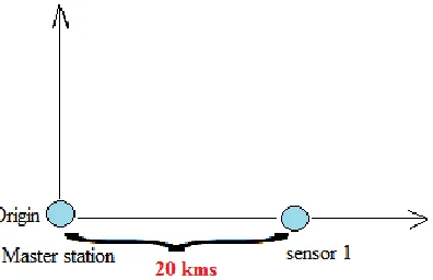
A Study of basic hyperbolic curve and its error analysis for a single baseline is carried out for which a master station is assumed at the origin (in principle any sensor can be considered master station) and the other sensor is considered along the x axis (single variable with y=0 and z=0).

[image:2.612.349.547.261.389.2]

Consider a basic study with the Master Station at origin and the other sensor at a position of 20kms along the x axis with zero measurement error as shown in the figure below.

Figure 2: Single Baseline Sensor Configuration.

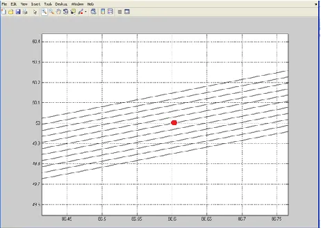
According to the hyperbolic position fix technique[4], the time difference computed between the pair of sensors produces locus of a hyperbola with the sensors on its focal points and the emitter on the hyperbola as shown in the graph below:

Figure 3: Graph showing the Emitter position on hyperbola for single Baseline Sensor Configuration.

IV. SIMULATION OF ERROR ANALYSIS FOR VARIOUS

SCENARIOS

[image:2.612.326.565.474.605.2]

(3)

International Journal of Emerging Technology and Advanced Engineering

195

A. Geometry of the Receiving Units

[image:3.612.329.560.176.340.2]

The geo-location of the emitter is computed using the time difference between the sensor pair. Since, the target is assumed to be varying so does the tdoa and therefore the computed range difference for a given sensor deployment or the receiving units[5]. This phenomenon and its effects on the target estimation is depicted below for the previous mentioned baseline.

Figure 4: Error Analysis of Single Baseline sensor Configuration for different Emitter positions.

Consider the case where the emitter is at the position E. The master station is at A and the other sensor is at B. Mathematically, the range difference can be computed as

AB=AE-BE,

but as the emitter E and the sensors lie on the same line, the signal is received by the sensor A later than the sensor B. In this case the hyperbola gets converged to a straight line. Consider the case where the emitter is at the position E’, which makes an angle where the range difference AB=AE’-BE’ =0, giving rise to a straight line perpendicular to the base line on which the emitter can lie.

B. Timing Accuracy of the Receiving Units

The Arrival time of a signal at the sensors is measured for computation of tdoa. The arrival time of a signal is actually the sum of time at which the transmitter emits the signal and the travel time. The arrival time is assumed to be altered due to factors such as reflections from objects etc, since the receiving unit has no information about the travel time or the emitting time of the signal. So, these alterations are eventually depicted in the tdoa and finally affect the positional accuracy for geo-locating the Emitter.

The below graph shows how the alterations in tdoa by ± few tens of nano seconds varies the hyperbolic curves and the region of locating the emitter.

Figure 5: Graph showing a magnified view of the behavior of the hyperbolic curves for tdoa Alterations.

The red dot is the emitter position and the magnified view of the hyperbolic curves above and below the actual one, is a result of the altered tdoa in steps of ± 10 ns respectively. The above graph shows a positional error of

150mts for an error of 50 nano seconds

.

V. SIMULATION OF 2DPOSITION FIX

The emitter location is determined from the

measurement of time difference of arrival (tdoa) between a pair of sensor units. Each tdoa and the sensor coordinates when manipulated mathematically produces a locus of hyperbola. Similarly manipulation of an another sensor pair and its tdoa produces another locus of a hyperbola with the emitter possibly lying on the intersection of these hyperbolas.

The behavior of the emitter region in case of zero and few tens of nano seconds of tdoa errors for different sensor deployments is studied.

A. Study of Emitter Behavior For Perpendicular Baselines

[image:3.612.57.279.241.357.2]

(4)

International Journal of Emerging Technology and Advanced Engineering

[image:4.612.64.282.113.287.2]

196

Figure 6: Multi-Baseline(Perpendicular) Configuration.

[image:4.612.329.560.131.328.2]

The graph below shows the pair of hyperbolic curves obtained from the two perpendicular base lines, the curves in black are plotted between the pair of sensors at the positions (0,0) and (20,0) and the curves in green are plotted between the pair of sensors at the positions (0,0) and (0,20) the intersection between these curves occur at the emitter position represent by ‘*’ in red. The emitter is varied at an angle with 10deg step and at a range of 100kms .It is this intersection point where location of the emitter is fixed.

Figure 7: Graph showing the intersection of hyperbolic curves at various Emitter positions.

B. Error Analysis For The Perpendicular Baseline

[image:4.612.52.285.428.586.2]

An error of ± 10 ns is added to the tdoa measurement. The emitter is varied angularly in a step of 10 deg and at a range of few 100s of kms. This behavior of the emitter uncertainty is studied in the graph shown below:

Figure 8: Graph showing the variation of region of Emitter Presence

The above graph shows a marked increase in the uncertainty zone with increase in the error in time difference measurement especially radially. This also

shows that the error is minimum around 45, which is the

bisector of the two perpendicular base lines and increases

as the emitter comes in line with any of thebase lines.

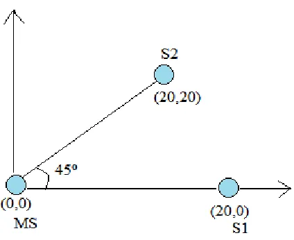
C. Study of Emitter Behavior For Tilted (Non-Perpendicular) Baselines

A configuration consisting of master station at the origin and a sensor 1 along the x axis at a distance of 20 kms and another sensor, sensor2 tilted at an angle with respect to the origin are considered.

[image:4.612.338.550.496.669.2]

(5)

International Journal of Emerging Technology and Advanced Engineering

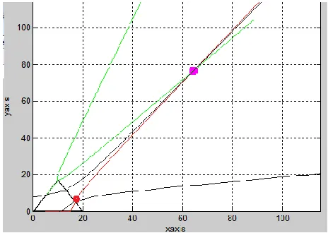
[image:5.612.338.551.149.277.2]

197 The graph below shows the behavior of the intersection region of the arbitrary baseline as the emitter rotates at an inclination of 10 deg step.

Figure 10: Graph showing the variation of Emitter region for non-perpendicular Baselines.

The region of uncertainty is observed to be minimum as the emitter makes an inclination close to the angle of the arbitrary baseline.

The Elliptical Error Probability(EEP)[6] is the uncertainty zone depicted above which is either due to geometry of the sensors or alterations in the tdoa or both. Hence when multiple sensors and multiple base lines are used, appropriate base lines and time differences have to be established to minimize the positional error while computing for location fix.

VI. MULTI-BASELINE POSITION FIX IN 2D

As discussed in the previous section intersection between the hyperbolic curves computed using the time difference is likely to be the emitter region, but the simulations have shown that the intersection is likely to occur at more than one region giving ambiguities in the detection of Emitter presence. Establishing another Baseline and computing its hyperbolic curve can be considered as a solution to eliminate this Uncertainty[6].

[image:5.612.50.289.174.357.2]

This phenomenon is explained using the sensor configuration shown below, with master station at the origin and the other sensors placed arbitrarily at an angle of 60˚ to the master station.

Figure 11- Three Baseline sensor Configuration to Eliminate uncertainties in Emitter region detection.

The graph below shows the simulation of this phenomenon where the red dot represents the ambiguity and the dot in magenta represents the emitter position as the curves from the three baselines intersect at that point.

Figure 12- Graph showing Location Fix for Multi-Baseline.

VII. SIMULATION OF 3DPOSITION FIX

[image:5.612.327.559.358.523.2]

(6)

International Journal of Emerging Technology and Advanced Engineering

[image:6.612.67.273.209.377.2]

198 A sensor deployment consisting of mater station at the origin and S1 at 20kms along the x axis, sensors 2 & 3 at arbitrary angles are considered. The configuration shown below is fixed for obtaining minimum positional error in locating the emitter after carrying out a thorough study taking the above mentioned error factors into consideration.

Figure 13: Multi-Baseline Configuration for 3D Location Fix.

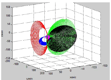
The graph below shows the intersection region of the hyperboloids computed between the sensor pair.

Figure 14: Graph showing the intersection of various hyperboloids at the Emitter region.

The dot shown in magenta is a region where there is high Probability of the Emitter Presence.

VIII. CONCLUSION

From the simulation analysis it is observed that the area where the emitter is statistically located is called the Elliptical Error Probability(EEP) where all the errors manifest themselves as EEP. In 2D, intersection region can be determined using two baselines, at most 3 are used for accurate location. Whereas in 3D 4 baselines are required to determine the region. However, increasing the number of receiving units would increase the accuracy of determining the region of emitter presence but comes at the expense of more ambiguities. The TDOA approach yields high LF accuracy of up to 250mts. The TDOA approach is useful for pulsed signals only.

Acknowledgements

The author wishes to acknowledge the Cooperation of Mrs. S. Sudha Rani, Sc-‘F’, of Defence Electronics Research Laboratory for her guidance on TDOA and its applications, and Mr.T. Venkata Rao, Associate Professor, Dept of ECE, of Sreenidhi Institute of Science and Technology for his valuable Suggestions.

REFERENCES

[1] Y.T. Chan, K.C. Ho, IEEE TRANSACTIONS on Signal Processing, Vol.42, No.8, August 1994, A simple and Efficient Estimator for Hyperbolic Location.

[2] John D. Bard, Fredric M. Ham, IEEE TRANSACTIONS on Signal processing Vol.47, No.2, February 1999, Time difference of Arrival Dilution of Precision and Applications.

[3] Hatem Hmam, DSTO, Edinburgh, Australia,2008, Passive Source Localization from time of Arrival measurements.

[4] Bertrand T. Fang, IEEE TRANSACTIONS on Aerospace and Electronic systems Vol.26,No. 5, September 1990, Simple Solutions for Hyperbolic and Related position fixes.

[5] L. Kovavisaruch, K.C. Ho, ICASSP 2005, Alternative Sources and Receiver Location Estimation using TDOA with Receiver position uncertainties.

[6] Melvin E. Shultz, USAF ,June 1963, Circular Error Probability a Quantity affected by Bias.

[7] Samuel P. Drake, Kuthuyil Dogancay, ICASSP 2004, Geolocation by time Difference of Arrival using Hyperbolic Asymptotes . [8] Erik Salva, Samantha O’ connor, Christopher Massa, Worcester

[image:6.612.50.286.423.594.2]